Article

A Decentralized Semantic Reasoning Approach for the Detection and Representation of Continuous Spatial Dynamic Phenomena in Wireless Sensor Networks

1
Centre de Recherche en Données et Intelligence géOspatiales (CRDIG), 0611 Pavillon Casault Université Laval, Québec City, QC G1K 7P4, Canada
2
GéoSémantic Research, Sherbrooke, QC J1L 1W8, Canada
*
Author to whom correspondence should be addressed.
ISPRS Int. J. Geo-Inf. 2021, 10(3), 182; https://doi.org/10.3390/ijgi10030182
Submission received: 24 January 2021 / Revised: 10 March 2021 / Accepted: 14 March 2021 / Published: 19 March 2021
(This article belongs to the Special Issue Applications of Discrete and Computational Geometry to Geoprocessing)

Abstract

:
In this paper, we propose a decentralized semantic reasoning approach for modeling vague spatial objects from sensor network data describing vague shape phenomena, such as forest fire, air pollution, traffic noise, etc. This is a challenging problem as it necessitates appropriate aggregation of sensor data and their update with respect to the evolution of the state of the phenomena to be represented. Sensor data are generally poorly provided in terms of semantic information. Hence, the proposed approach starts with building a knowledge base integrating sensor and domain ontologies and then uses fuzzy rules to extract three-valued spatial qualitative information expressing the relative position of each sensor with respect to the monitored phenomenon’s extent. The observed phenomena are modeled using a fuzzy-crisp type spatial object made of a kernel and a conjecture part, which is a more realistic spatial representation for such vague shape environmental phenomena. The second step of our approach uses decentralized computing techniques to infer boundary detection and vertices for the kernel and conjecture parts of spatial objects using fuzzy IF-THEN rules. Finally, we present a case study for urban noise pollution monitoring by a sensor network, which is implemented in Netlogo to illustrate the validity of the proposed approach.

1. Introduction

Wireless sensor networks (WSN) are increasingly used for monitoring and sensing dynamic spatial phenomena [1]. These networks, which are also referred as geosensor networks, are considered as remote sensing instruments deployed in the environment which provide observations of environmental processes at a spatial and temporal resolutions never seen before [2]. Sensors are able to locally sense phenomena in a continuous way, providing users with data of fine resolution to describe the behavior of dynamic phenomena on a near-real time basis [2,3]. Data collected by WSN are useful for a wide range of applications from social to urban dynamics and from transportation to healthcare purposes for informed decision-making [4,5,6].
Despite advances in the area of sensor technology, sensing devices are prone to some limitations and restrictions including sensing range, battery power, connection ability, memory, and limited computation [7]. Spatial computation from raw sensor data (RSD) can be undertaken in a sensor system following a centralized approach where all the data are sent to the central site, a decentralized approach where data stay at individual sensor sites or a hybrid approach [6]. In the decentralized approach, which stands as a solution to the limited capabilities of sensors, each node locally computes partial spatial information about the sensed reality from its measurements and those of its direct neighbors [8].
Most of the approaches developed for field-like phenomena are developed on the assumption that the boundaries of such phenomena are crisp, whereas many environmental phenomena such as dust, noise or gas pollution or forest fires have vague spatial boundaries [9]. Hence, it is generally not possible to directly detect the boundaries of monitored phenomena from sensor measurements [10]. This is because sensor nodes are either randomly dispersed over the monitored area or follow a particular pattern [11,12,13]. However, their location rarely coincide with monitored phenomena boundaries. Hence, we need collaboration among nodes to infer and aggregate knowledge describing the complete spatial extent of the phenomena. This process that implicates real-time assessment of a large amount of widely varying sensor data with inherent uncertainties for modeling field-based dynamic phenomenon is still a challenging problem [14]. Furthermore, if such a field-based phenomenon with vague boundaries is represented using a crisp spatial object, subsequent spatial computation (e.g., topological analysis) may result in poor decision-making process.
This article aims at improving representation of field-based spatial dynamic phenomena monitored by sensor networks, by fostering the extraction of vague spatial objects from sensor network observations. Here, we propose to integrate the semantics of sensor data, domain, and vague spatial models to build semantic rules for qualitative reasoning for the extraction of knowledge and representation of a field-based spatial phenomena. For this purpose, fuzzy logic theory is used to consider the inherent uncertainties in sensor data and spatial fuzziness of monitored phenomena to build a more realistic spatial representation of the phenomena. The proposed qualitative reasoning method benefits from Lukasiewicz’s three-valued logic, which is a case of fuzzy logic using three truth-values indicating true, false and some indeterminate third value [15], for dealing with problems of uncertainty in raw sensor data as geospatial data, in order to extract vague spatial objects representing the monitored phenomenon and its dynamics. The originality of this paper relies in solving the two levels of vagueness in computing the geometry of vague spatial objects in order to build a more realistic vague spatiotemporal model of monitored phenomena from distributed sensors observations.
The remainder of the paper is organized as follows. Section 2 presents an overview of related works and methods on spatial computing from sensor data as well as the inherent uncertainties related to the observation and representation of a dynamic phenomenon from raw sensor data. Section 3 presents the conceptual framework of the proposed approach for decentralized semantic reasoning for modeling vague shape phenomena. In this section we present in detail all the components of the framework and describe their formal representation. Section 4 presents a case study on urban noise pollution monitored by a sensor network, implemented in Netlogo software to illustrate the results of the suggested approach, which are then discussed. Section 5 analyses the results of the approach and draws out conclusions and perspectives for further works.

2. Related Works and Concepts

2.1. Spatial Computing in Sensor Networks

Sensor data express through their value, the presence or absence of a phenomenon at a given location (sensor position or its vicinity) and time (time point or time period) [16,17]. The values recorded locally by sensors characterize a phenomenon of interest and help to obtain information on its spatial and temporal extents. Computing spatial information from RSD to model phenomena can be performed using centralized or decentralized approaches. In centralized approaches, sensor nodes are used as data collectors. Collected RSD are all transmitted to a sink node, where data processing can be undertaken, as shown in Figure 1.
In such system, sensors generally operate following a ‘sense-and-transmit’ approach [18] maximizing the communication load of sensors over the sensor network [2]. In a sensor node, energy is a vital and limited resource. Such energy is consumed for sensing, communication, and data processing activities. Because energy is mostly consumed for data communication [4], a centralized spatial computing approach limits the life span of sensors over the WSN. In centralized approaches, only the sink node undertakes spatial computing. Computed information is reported as successive spatial snapshots of monitored phenomena. No sensor node of the WSN, apart the sink node, computes spatial information about a monitored phenomenon.
Decentralized approaches attempt to solve some of these limitations by allowing sensors synchronously collaborate with their neighbors, using a communication network, to compute spatial information on monitored phenomena. This information includes local statistics, filtering, or qualitative reasoning on RSD. Taking advantage of their onboard computing capabilities, sensing devices can detect the presence of phenomena and, based on their neighbors’ measurements, they can help to detect and infer object boundaries for the spatial modeling of phenomena and their dynamics [2].
Several decentralized approaches have been developed for the detection of spatial boundaries. Two main categories of these approaches include 1) filters and statistical techniques for spatial computations on RSD and 2) qualitative reasoning approaches for spatial computations on RSD. Nowak and Mitra [19] and Chintalapudi and Govindan [20] are examples of the statistical approaches. Nowak and Mitra [19] propose dividing the observation region on which the WSN is deployed into a regular grid with a sensor in each cell. The proposed method reasons on the presence of the phenomenon boundary by performing statistical analysis over RSD recorded in the cells to detect areas of high variation around thresholds. Areas of high variation are considered as boundary zones of monitored phenomena. Irregular spatial distribution of sensor nodes within the sensor network extent remains a problem in this approach. Chintalapudi and Govindan [20] used the idea of abstract regions (areas within a radius around a sensor), and applied specific processing (statistics, filtering, and classification) on RSD using threshold values within each region to predict the boundary vertices. This idea was used by Welsh and Mainland [21] to improve computing activity in SN in the vicinity of detected boundaries. This approach shows high sensitivity to high variation in readings, the presence of imperfections (outlier due to measuring errors), the choice of the threshold and the network density.
In qualitative approaches, the reasoning on RSD generally indicates whether the phenomenon of interest is present or not at a given position and time. In some cases, phenomena detection is established using thresholds applied on sensor record values [22]. For a given sensor (S) at a position (p) in a WSN, a sensor data RDS (p,t) produced by S at time t implies the detection of the phenomenon A(p,t)=a, where a is a qualitative value expressing its occurrence as presented in the following expression:
R D S p , t A p , t =   a ,   i f   R S D p , t α   O R   a ,   i f   R S D p , t < α N o t   a ,   i f   R S D p , t < α   O R   N o t   a ,   i f   R S D α
where α and α’ = threshold values
For illustration, the use of a temperature threshold α 200 °C may help in fire detection [23]. Also, water PH value of α <6.8 or α’ >9.5 may be used to detect poor water quality [24].
Among these approaches we can mention the work by Guan and Duckham [25] where each sensor node detecting the phenomenon sends queries to its one-hop neighbors if they detected the phenomenon. Each node reasons from the answers to its queries to infer the phenomenon boundaries. In their approach, each node has a status coded on 2 binary digits where the first digit expresses the detection of a phenomenon and the second, the detection of the phenomenon boundaries. These sensor statuses help in modeling the spatial extent of a phenomenon and extracting information on its evolution and topological relations with other phenomena [8,25,26].
Despite the performances shown by these approaches, high range variability in sensor readings particularly between the interior and the border of a phenomenon still cause major problems in accurately detecting boundaries of monitored phenomena [27]. Furthermore, these approaches are developed on the assumption that monitored phenomena have a defined boundary. This is not always the case in spatial dynamic and continuous phenomena, and may lead to poor detection and modeling of a phenomenon and its dynamics, and consequently to poor decision-making.

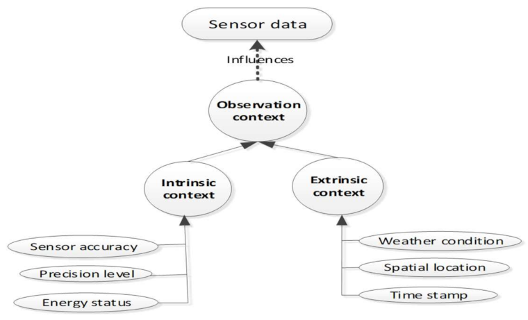
2.2. Sensor Data Geosemantics

Wireless Geosensor networks help to remotely measure physical properties of phenomena of interest in order to detect their presence at a given area [2]. Each sensor can measure one or several properties (temperature; emission of CO2, CO, NO2, SO2, H2CO etc.; rain fall; humidity …) of one or several phenomena (climate conditions: sunny, rainy…) [17].
Extracting geospatial information from sensor data may then be influenced by the spatial nature of monitored phenomena (fuzzy or crisp) and the semantics specifications of sensors and as well as the network itself. While semantics describes the meaning of sensor data, the observation process depends on sensor technologies used for the measurements [28,29] and their deployment in the study area (hazardous and irregular or following a pattern) [11,12,13]. Such supplementary information on sparse or dense fine-grained RSD are relevant in computing spatial knowledge from RSD and assuring seamless collaboration among networked nodes to reason and model large-scale phenomena such as bushfires, air pollution, floods, etc. is essential [30,31]. For example, there are different ways of measuring temperatures. Procedures can describe so-called contact-based methods, e.g., based on the expansion of mercury, or contact-free methods such as infrared thermometer. The sensor position, which may be different to that of a feature of interest (FOI), cannot be considered similar in these two cases while computing spatial information about the FOI. Meaningful spatial information is obtained using different reasoning approaches (semantic, statistical, etc.).
In the perspective of decentralized spatial computing, sensors are considered intelligent agents [8]. They are able to compute spatial information from their observations and measurements and collaboratively build a realistic geospatial representation of the monitored phenomenon. In such a context, bridging the gap between raw sensor data and abstract domain knowledge is the main challenge in preparing the reasoning engine of sensing agents for the extraction of the knowledge on a field-based spatial phenomenon and its spatial representation.

2.3. Inherent Uncertainties Related to the Observation and Representation of a Dynamic Phenomenon from Rsd

Stasch et al. [17] argued that sensor data are proof than the fact itself. Sensor data provide information about some properties of observed phenomena, which in most cases are not tangible. According to the classification of property types by Kavouras and Kokla [32], the properties observed by sensors may not be “characterizing properties”(i.e., which can be used to partition the world into specific things) and cannot help in identifying the occurrence of phenomena with strict precision. For instance, in the case of a wildfire, smoke can be detected all around the area under fire. Also, the propagation of heat can lead to high temperatures around the fire. Using these properties to model the area under fire should not be considered with the same level of certainty as detecting flames. Then, modeling a wildfire phenomenon using sensor data related to temperature measurements with a crisp spatial object may not be appropriate. In order to overcome the limitation of such representation, fuzzy–crisp object model [33], made of a kernel part and a conjecture part is a good candidate. The kernel part definitely and always belongs to the vague object, but one cannot say with certainty whether the conjecture part belongs to the vague object [34]. The five (05) topological parts constituting such a simple fuzzy region, as identified in [35], are presented in Figure 2
Considering the example of a wildfire, Figure 3, shows the crisp and fuzzy–crisp representations of a wildfire event. In this figure, the red-colored area expresses the presence of very high temperatures (flames) while pink color stands for an area with high levels of heat (higher than ambient temperature but less than flame temperature).
In addition to the vague nature of many environmental phenomena, which complicates their consistent detection and representation, RSD may be semantically poor [36] and prone to some uncertainties associated with calibration or sampling effects (discrete sampling of the measurements or measurement errors) [37]. This may also contribute to incomplete knowledge or poor detection and representation of spatial phenomena and their dynamics [38] using sensor networks.
In addition to the spatial fuzziness of monitored phenomena, the varying sensing range of sensor nodes and their location, which rarely match with the boundary of monitored phenomena, hamper the computation of the spatial extent of the phenomena from sensor measurements. In such process, the communication network supports the collaboration among sensors (Figure 3). In a low-density context, where there are too few neighbors around a given sensor node, that sensor node may increase the communication range [39]. In such situation, the vertices of a given edge may be too close or too far from the position of sensors detecting this edge (see Figure 4). Using sensors position as edge vertices may be inappropriate for a certain number of applications. For instance, it may be risky to use inner sensors position as vertices delineating a fire zone extent, leading to a poor firefighting strategy.
Based on Molenaar [10] works, we identify three conceptual uncertainty levels for spatial objects extracted from sensor data as follows:
  • The existential uncertainty expressing how sure we are that a given phenomenon really exists at a particular position in space and time from recorded sensor data,
  • The extensional uncertainty expressing how the area covered by the monitored phenomenon can only be determined,
  • The geometric uncertainty refers to the precision with which the boundary of the object representing the monitored phenomenon can be detected.
Jadidi et al. [40] propose a comprehensive diagram of uncertainty in spatial data modeling. Fuzzy set theory originally proposed by Zadeh [41] can be used to evaluate the membership of a given sensor node values in a specific location and time to a monitored spatial phenomenon. However, evaluating the membership value of a given RSD requires a fuzzy membership function (MF) which definition (shape) is not an easy task [42] and should cope with the meaning of RSD, the semantics of the adopted spatial model and that of the application for which modeling is undertaken. In brief, from the bottom level (sensor node) where sensor data are collected and translated into spatial information, to the top level (sensor network) where the fuzzy spatial object representing a monitored phenomenon at a given date is built, there are some challenges in preparing the reasoning engine of sensing agents. These include: (1) defining the appropriate membership function used by sensors to change collected data into fuzzy sets, (2) ensuring meaningful integration and communication among sensors by deriving semantic rules from ontologies to translate sensor data into geospatial information, and (3) handling geometric uncertainties in inferring vertices from sensor collaboration to define the geometry of the spatial object representing a sensed phenomenon.
To address these issues, we propose a new approach in computing and modeling vague shape spatial phenomena in WSN using a decentralized semantic reasoning process for building snapshots of fuzzy-crisp spatial type from sensor data. The suggested approach is presented in detail in the next section.

3. Building Vague Spatial Objects in Sensor Networks Using A Decentralized Semantic Reasoning Approach

Here, we propose a semantically enabled decentralized fuzzy rule-based method for the extraction of vague spatial objects from sensor data. The proposed method has three main components (Figure 5), including:
1.
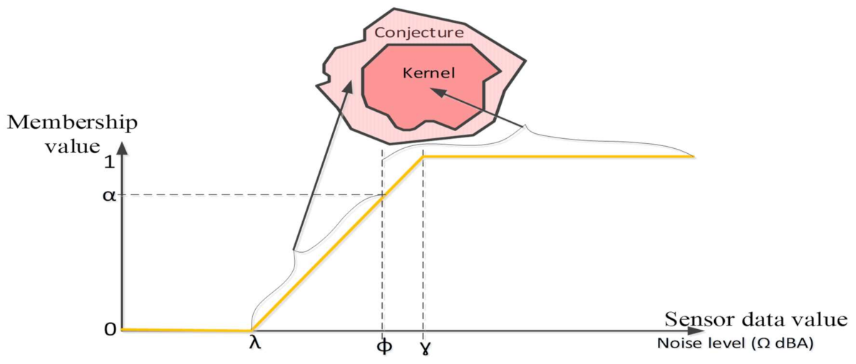
Fuzzy rule-based detection of a monitored phenomenon: here, sensor nodes use a built-in reasoning engine to evaluate the membership of their location to different parts of the spatial extent of a monitored phenomenon using a MF and the observed data at a given time. The MF shape and definition need to cope with the semantics of sensor network data, the phenomenon and its spatial model. Defuzzification rules based on three valued logic are also set accordingly.
2.
Decentralized fuzzy inference of spatial boundaries of a monitored phenomenon: each node collaborates with one-hop neighbors based on their phenomenon detections and the semantic of adopted spatial model to infer their relative position to phenomenon boundaries.
3.
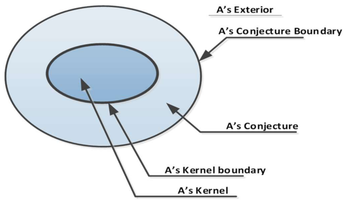
Spatial computation of vertices, edges and geometry of monitored phenomenon snapshots: using the relative positions of linked nodes to detect boundaries, vertices, location, and categories (kernel or conjecture) are determined. Fuzzy boundary edges are built based on vertices position and categories, forming the geometry of spatial objects representing phenomenon snapshots at a given time.
In the following sections, each of the components is presented in detail.

3.1. Fuzzy Rule-Based Detection of a Sensed Phenomenon from RSD

This component aims at providing sensor nodes with the ability to infer the detection of a particular phenomenon based on sensor data according to the semantics of the phenomenon and the adopted spatial model. This is locally done at the sensor level by a reasoning engine. The integrated reasoning engine is made of logic and semantic rules and a membership function (MF) used in solving the issue of vagueness in sensor network data and the fuzzy nature of the monitored phenomenon, in order to produce a realistic spatial representation of the monitored phenomenon. This is a two-stage process. The first stage is devoted to the preparation of the inference engine with the definition of the fuzzy membership function, logic and semantic rules (semantic integration of sensor network data, domain ontologies and spatial model), and defuzzification rules. Stage 2 is devoted to the computation of spatial information related to sensor data collected following the sampling procedure. Collected data are transformed into fuzzy sets using the membership function. Issued fuzzy data are then translated into qualitative spatial information (kernel, conjecture (a broad boundary) or out) using reasoning logic and semantic rules.

3.2. Stage 1: Preparing the Sensors Reasoning Engine

We describe here the different activities carried out to prepare the reasoning engine equipping sensors, as presented in Figure 5.
  • Knowledge base and rule base preparation
To build a knowledge base at the sensor level in order to help sensors to automatically translate their measurements into geospatial information, we mobilize semantic features from:
A sensor ontology such as the semantic sensor network ontology (SSN) [43], from which the meaning of sensor network data can be explicitly specified. This is the case of the observation procedure, which defines the way sensors execute its measurements.
A domain ontology designed for describing particular domain entities or a certain activity [44], from which the monitored phenomenon can be explicitly interpreted or represented from sensor observations.
In our approach, we suggest the selection of appropriate fragments of sensor ontology and domain ontology in accordance with the phenomenon of interest and its spatial representation, in order to build a light knowledge base at the sensor level in a sensor network. Methods such as IF-Map which basic principle is to match local ontologies to a common reference ontology [45]. IF-Map produces concept-to-concept and relation-to-relation alignments formalized in terms of logic infomorphisms denoting information flowing between these ontologies and making the common reference ontology [46,47]. According to Kalfoglou and Schorlemmer [47], the result of this mapping is based on appropriate fragments (token) of the considered ontologies (sensor network, domain) to ease the mapping procedure as shown in Figure 6.
In the mapping procedure, the sensor type specified for phenomenon observation in the domain ontology is a sub-type of sensor in the ontology. Observation location that corresponds to sensor location is the base for modeling phenomenon spatial extent through simple regions, which may be different sub-types: crisp, vague or completely vague (made only of conjecture) region. The mapping relationships are established using semantic rules. The set of rules forming the rule base of the reasoning engine is developed to ensure the translation from sensor data values to qualitative spatial information based on semantic specifications expressed by ontologies. These semantic specifications are formally presented as logic rules predicating how sensor data describe the observed properties of a monitored phenomenon and its spatiotemporal behavior.
Sensors records are mostly made of values describing a property of a given phenomenon at a given time [48]. Logic rules and infomorphism derived from integration of domain ontology into sensor ontology define how sensor data subsumes phenomenon feature. Ontology mapping is formally expressed using semantic rules. Sensor data (position, time, value) characterize the phenomenon of interest. Before computing spatial information from sensor data, the reasoning engine assesses their validity to avoid outliers or mismatch interpretation. The validity of sensor data describing observed phenomenon can also be assessed through logic rules, as follows.
valid_data (Sensor_ID,Time_reading,Value):
  • sensor_type (Sensor_ID, Sensor_model, Measured_Propert, Unit),
  • sensor_range_value (Type_model, Minvalue,Maxvalue),
  • phenom_sensor (Type_phenomenon, Sensor_model,Pehnom_prop),
  • Value ≥ Minvalue, Value ≤ Maxvalue.
Context awareness in pervasive computation systems such as in sensor networks is of great importance [49]. The context in which observations and measurements are undertaken at any given position in a sensor network influences the meaning of sensor data for a specific use. The context of observation describes conditions which are either intrinsic or extrinsic to sensor nodes, as illustrated in Figure 7.
Intrinsic context includes all sensor-dependent factors (as sensor accuracy, record precision, energy level, etc.), which can influence sensor data values resulting from observations. Extrinsic factors are not sensor-dependent, for example, the weather conditions during measurements. For instance, a sensor measuring wind speed may have a level of accuracy of ±3km/h in raining conditions and a level of accuracy < 1% of this value in sunny conditions. This should be considered while making use of RSD.
  • Setting the fuzzifier unit
The use of a membership function (MF) determining the degree of belonging of an element to a set is essential to infer on the detection of vague objects from the set of RSD collected by a sensor network. The MF is considered by Yazici et al. [50] as a generalization of the characteristic function. Its definition should cope with the semantics of the phenomenon and the application for which the detection is intended. The shape of a MF can be sigmoid, triangular, trapezoidal, Gaussian, Pi, S, or Z shaped [51]. The shape and parameters of the MF are defined in accordance with the characteristics of a given phenomenon [52].
For illustration, let us consider sensors recording noise levels in decibel (dBA) within the vicinity of a given source, knowing that the basic noise pollution emitted is < λdBA, the background maximum noise level in the area is φdBA and that the minimum noise level produced by a given source is ɣdBA with ɣdBA > φdBA. The detection of a noise level ΩdBA for which the value is defined as φdBA ≤ ΩdBA ≤ ɣdBA at a given position can be identified as polluted by the considered source of noise. The membership of such record as polluted by this source is 1 whereas a record defined by ΩdBA < λdBA has a membership of 0. The MF generalizing such case can be of S shape as presented in Figure 8, where α is the admitted membership value of noise for a given location.
  • Setting the defuzzifier unit
As we mentioned in Section 2.3, the spatial vague object we envisage as model is composed of a kernel part and a broad boundary called conjecture. Based on the sensed data, the reasoning engine should be able to infer whether a sensor is within the kernel or the conjuncture part at a given time. Such information may help to describe the internal structure of the uncertain parts of spatial objects with vague shapes [53]. There is a need to translate this membership values into a truth value, expressing the spatial relation (within) between the location of sensor nodes and our vague spatial object representing the phenomenon.
The knowledge base and rule base set of statements, as the fuzzy membership function and defuzzification rules, are formally expressed as basic instructions that can be implemented by the computing unit of any single sensor. These instructions are compiled and integrated into sensor nodes. Their content is updated by collected data from which spatial information is inferred. This set of formal instructions constitutes the built-in engine used by any sensor to reason in order to contribute to the spatiotemporal modeling of the monitored phenomenon.
Using a membership function transforms sensor data into fuzzy sets.

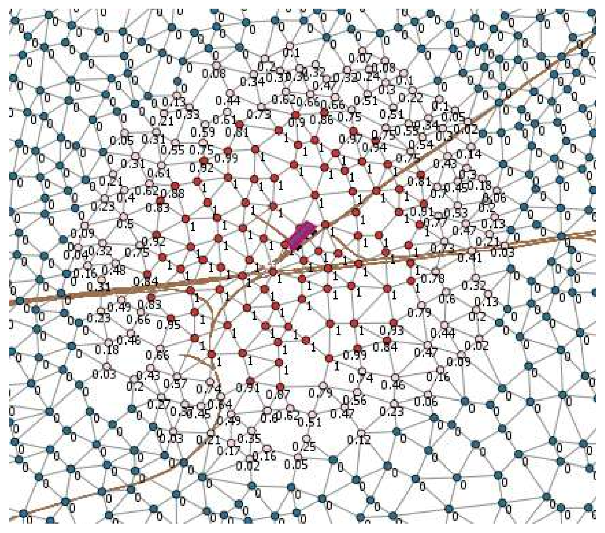
3.3. Stage 2: Fuzzy Spatial Reasoning from Rsd: Fuzzification and Defuzzification Processes

Sensors generate a flow of data from their measurements over time [54], following a sampling procedure implemented by the sensor. Each measurement triggers the computation of new qualitative spatial information that assigns a spatial status (kernel position, conjecture position or outer position) to the very sensor node.
The membership function is used to assign a membership value to input values, changing the set of raw data into a fuzzy set [55]. For a given sensor (S_i) recording the value Sr(t,Loc(S_(i ) ) → (Val,t,Loc(S_(i))) at time t and location Loc(S_(i)), if the membership function f(Sr):Sr → [0,1] expressing the membership of a given record about a phenomenon by a value μ∈[0,1]. Fuzzification consists of changing the set of recorded sensor data into a fuzzy set which membership value will be used for defuzzification and spatial computation.
According to the membership value of a sensor record, the position of a sensor node can be within the spatial object or not at a given time. For the defuzzification procedure, we use the three-valued logic to express this ”within” spatial relation between the sensor location and the phenomenon extent. Defuzzification results in reducing a fuzzy value (raw sensor data) to a crisp single-valued quantity, or to a crisp set, making them understandable for spatial reasoning [40]. Reducing this RSD set into a set of spatial qualitative values expressing the relation Loc(S) is within Vobj (Vobj being the vague object representing the phenomenon) correspond to a three-valued logic, as presented in Table 1.
Considering the position of each sensor location vis-à-vis the foreseen vague object, we assign a status to each node: Kern if it is in the kernel part, Conj if it is in the conjecture part and Out if it is outside.
Information about measurement conditions (measurement period (diurnal, nocturnal, sunny, rainy: extrinsic context) is relevant for computing spatial information by sensors. For instance, the threshold value specified in respect to a given phenomenon may change according to the measurement context. For example, in the case of noise pollution, nocturnal and diurnal records will be differently interpreted as part of the extent if the admitted level of noise pollution during the night is less than that of daily time. The sensor clock may help in differentiating diurnal from nocturnal measurements while other sensors may be required at a given node for weather conditions.

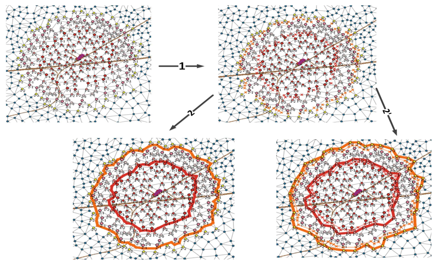
3.4. Local Collaborative Spatial Reasoning for Boundaries Detection Using a Geosensor Network

Boundary recognition from RSD is a key aspect in modeling monitored phenomena [56]. Each sensor in the network can sense without being able to directly detect the boundaries of the phenomenon. In previous works [8,57], by collaborating with its one-hop neighbors, each sensor can infer on its relative position in relation with the phenomenon boundary. Sensor locations rarely coincide with a phenomenon boundary. A sensor location will be close to a phenomenon boundary by the interior if its location is within the phenomenon extent and one of its closest neighbors is out of the phenomenon.
A fuzzy-crisp object, as vague spatial object representing an uncertain spatial phenomenon, is made of a kernel part and a conjecture part (Figure 3) [58]. The kernel part definitely belongs to the vague object. However, one cannot say with certainty whether the conjecture part belongs to the vague object [34]. The conjecture part of a vague spatial object constitutes the broad boundary of this vague spatial object [59]. In our approach, for a phenomenon with a broad boundary, a given sensor, may have one of the seven possible relative positions presented in Table 2. As it is the case in decentralized spatial computing, individual nodes do not have access to global information, which is considered as the top-level spatial information, but only to basic local information assumed to include their own state and those of their immediate (one-hop) neighbors.
A sensor detecting a phenomenon (kernel or conjecture) sends queries to its one-hop neighbors named N(s) through the communication mesh (Gabriel Graph [60]) materialized by links between nodes, as shown in Figure 9. Nodes sending queries provide each of their respondents with the required information: identification, location, inferred spatial status at a given time. The general form of the query is as follows:
Type_Query: My_Id=ii, My_loc = xy, My_detection=type, Time =tt, ?Your_location, ?Your_detection
There are two types of queries propagated in the network, KQuery and CQuery for queries with My_detection = Kernel and Conjectue respectively. On this basis, each respondent or query node can be deduced from the set of queries or answers received whether its position is a kernel or conjecture boundary position; if so, each node determines its relative position with respect to the kernel or conjecture boundary as shown in Table 2.
By querying one-hop neighbors about the detection of an observed phenomenon at their positions, each sensor node will infer its membership to one of these seven spatial categories using reasoning rules applied on the set of answers to its queries. For example, a node with a kernel position which receives only queries of type KQuery, will have a kernel inner position while the reception of CQuery will result in an inner-kernel-boundary position. These reasoning rules are integrated in the reasoning engine of each sensor. As formerly said, the positions of sensors rarely match the vertices of a phenomenon extent. Inferring the vertices (kernel and conjecture vertices) is essential for computing the kernel and conjecture boundaries describing the geometry of the fuzzy object representing the observed phenomenon.

3.5. Spatial Representation of Sensed Phenomena in SN: Vague Object Geometry

The spatial locations of sensor nodes S, with their membership value and spatial categories can be considered as fuzzy point sets. The point set concept has been widely used in spatial analysis [61,62] and geometric modeling of spatial objects [63]. From the border detection, out of 7 sets previously discussed, 4 sets of nodes (those detecting boundaries) are pertinent for the determination of the geometric boundaries of the fuzzy spatial object, representing the snapshot of the monitored phenomenon at timestamp t :
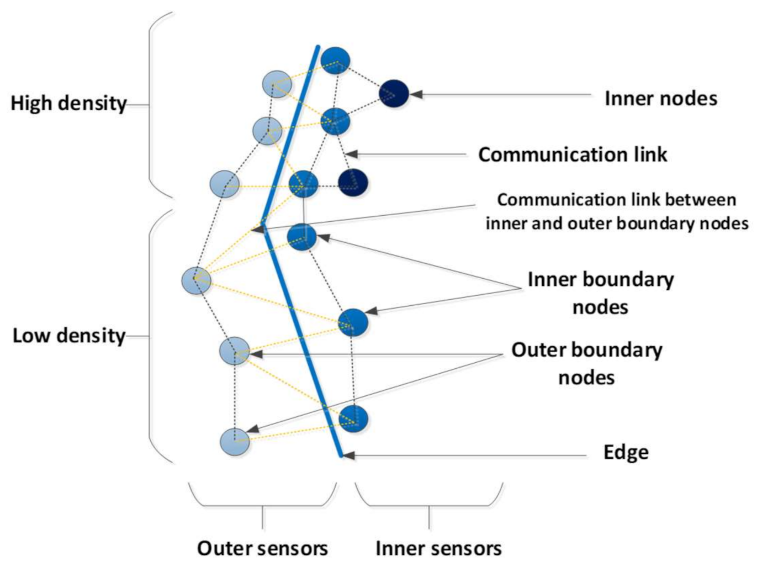
  • Inner kernel boundary nodes, noted: S 1 1
  • Outer kernel boundary nodes, noted: S 1 2
  • Inner conjecture boundary nodes, noted: S 2 1
  • Outer conjecture boundary nodes, noted: S 2 2
Partial and uncertain spatial knowledge of sensor nodes is known to be a particular characteristic of SN [8], each sensor can only be aware of the situation at its location and vicinity but not of the entire network extent. A node detecting the monitored phenomenon can guess border detection but will not identify boundary vertices with certainty. Instead of the lower and upper approximations promoted in [64] as a response to such uncertainty, we suggest a weighted approximation rule. Then, the three approaches are summarised in Table 3. The choice of a rule depends on the nature of a monitored phenomenon and modeling purposes. Decision-making is made based on the process of sufficiently reducing uncertainty and doubts about alternatives allowing a reasonable choice to be made among them [65]. For instance, in a case of bushfire disaster management, modeling for safety and evacuation strategy can be based on the lower method whereas modeling for firefighting strategy can use the upper method.
The weighted approach (based on inner, outer positions of nodes and distance among them) can use one of the two rules: 1 (based inner position) or 2 (based on outer position) where: μ I n n e r > μ O u t e r .
For each sensor, which position is close to the boundary of the Kernel S 1 1 ; S 1 2 , or conjecture part S 2 1 ; S 2 2 , the vertices for the kernel or conjecture parts are identified based on a certain number of parameters among which:
  • its membership value μ s i j with μ s 1 1 > μ s 1 2 > μ s 2 1 > μ s 2 2 ;
  • the set of one-hop neighbors with different position type (inner - outer) along the same boundary n b r s i j = s i j | j = j ± 1 E ;
  • the distance to these one-hop neighbors of other type d i s t s i j s i j s i j , s i j with dx and dy the x and y components of the distance.
A vertex of the kernel boundary of a fuzzy-crisp spatial object is somewhere along a link L s 1 1 , s 1 2 . This is illustrated in Figure 9 where kernel boundary vertices are represented by red cross signs at midway of L s 1 1 , s 1 2 links and conjecture boundary vertices using orange cross signs along L s 2 1 , s 2 2 links. These two sets of vertices are connected clockwise or anticlockwise, based on their position, to form kernel or conjecture boundaries. A case of weighted approximation is presented in Figure 9.
The formal presentation of the approach is broadly provided in Box 1 as pseudo-code.
Box 1. The pseudo-code of the proposed approach for extracting vague spatial objects from sensor data.
Detection and monitoring of dynamic phenomena
Variables: SN={s1,s2,…,sn}; a sensor network made of n nodes
S-On, D-On; a sensor ontology, a domain ontology
RSD={(s1,t,val1),(s2,t,val2),…, (sn,t,valn)}; a set of sensor data collected at time t
Context: Context (RSD): the context specification of observation
Functions:
MF; a membership function computing the membership value of sensor readings
Begin
Step1: fuzzy rule-based detection of dynamic phenomena; step1 is made of 2 sub-steps
Substep1: Building the knowledge base (formal transcription of ontologies assertions and context semantic rules)
Initializing sensor records and status; emptying all the variables assigned to each sensor
Substep2: Fuzzy reasoning from sensor data (sensors compute qualitative spatial information from their records, using membership function and semantic reasoning)
Step 2: Decentralized fuzzy reasoning for boundary detection; identifying sensor nodes with a bordering position of the spatial object parts
Sensors detecting the phenomenon, formulate appropriate queries and sent them to their direct linked nodes.
The detection of boundaries positions is done based on the set of queries or answers received
Sensors with boundaries position infer on vertices for the kernel and conjecture parts
Step 3: Spatial modeling of detected phenomena; vertices determination for kernel and conjecture
building boundaries of the parts (kernel and conjecture) of the spatial object representing the phenomenon
End.

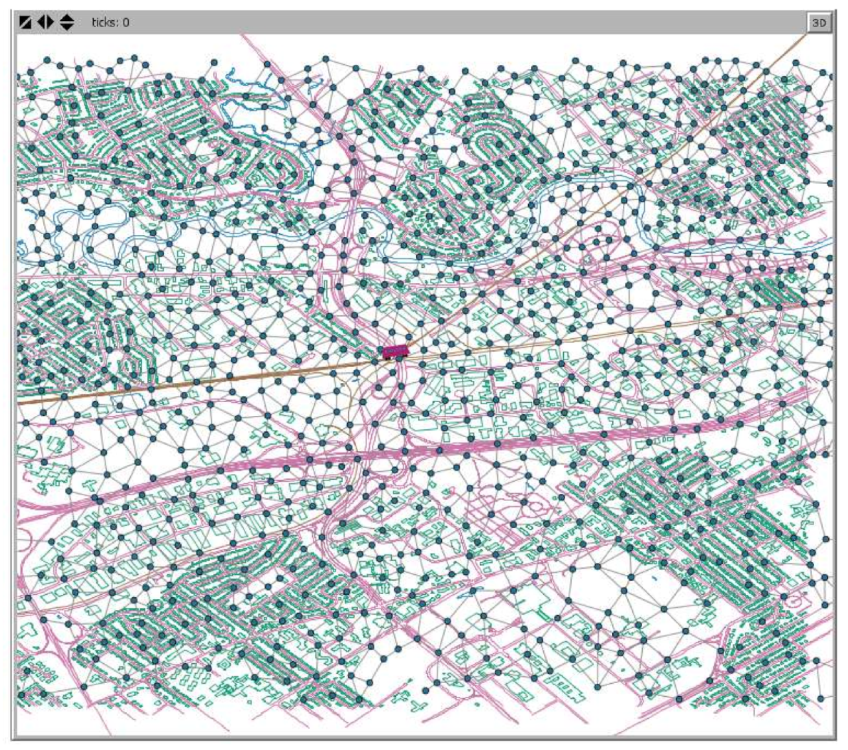
4. Case Study: Monitoring Noise Pollution Caused by Railway Activities in Quebec City

To demonstrate the validity of the proposed approach, in this section, we present a case study for modeling noise pollution in Quebec City from sensor data. Disputes related to noise pollution in large cities are of major concern where ambient noise sources may be localized in space and time (e.g., noise from a factory or aircraft flyovers, traffic on nearby roadways) [66]. Sound level meters (sonometres) help in evaluating the noise level at given positions, thereby evaluating noise pollution according to different purposes (e.g., civil interest or conflict resolution). Sonometers are mostly installed in fixed positions within a non-regular pattern, mostly following the location of potential sources (railway, road network, airport, factory, etc.). The level of sound pressure decreases as the distance to the source increases but not linearly. The presence of obstacles also modifies the noise level at a given position [66,67]. In most cases, noise pollution is evaluated according to its influences on human health with a level of noise pressure of less than 40 dB as recommended by the WHO for noise safe environment. The Canadian Transportation Agency (CTA) estimates the background noise level varying from 70dBA in noisy urban areas to 50 dBA in quiet suburban residential areas. Determining if railway activities producing up to 100 dBA is the main source of noise pollution in a city may depend on the community type (commercial or residential) which cannot be differentiated with crisp boundaries.
  • Setting a model in Netlogo for the detection of noise polluted areas due to railway activities
For this case study, we have used a geospatial dataset of a part of Quebec City in Canada. This dataset includes features such as buildings, roads, railways, along with their descriptive data obtained from the open spatial database of Quebec City (https://www.donneesquebec.ca/). Instead of an optimized spatial coverage of sensor network which is required for many urban applications [68], we have simulated a dense network of sonometres in order to capture noise pressure around a railway for train activities. We assume that the distribution of the devices corresponds to the standards used for this type of application. This was done using Netlogo (a GIS extension) which is a free multi-agent-based modeling application [69].
Figure 10 shows the selected area of Quebec City. In this figure, the roads are shown in violet, railways in brown, buildings in turquoise and rivers in blue. We suppose the presence of a train in activity on one of the railways, propagating noise in the surrounding environment, while sound meters are represented in blue with a ”mote” shape. Sound meters in the vicinity of the train in activity record a more important noise pressure. All sound meters can be labeled with the level of noise they record at their location.
Here, we focus on the production and propagation of noise during the motion of locomotives. The maximum noise produced by the locomotive is set to 100 dBA as evaluated by the CTA [66]. We consider that the level of noise expanded in the vicinity of train activity decreases linearly with the distance in a radius around the train during its trip.
Extraction of the noise polluted areas around railway activities.
In this case study, we consider a minimum noise level produced by train in activity of 70dBA and the little additional noise added to the background noise is 50 dBA is for a residential zone. According to this description, a membership function named Membdegre with a simple S shape function is set to compute the membership value of each recorded RSD. The expression of Membdegre for Netlogo Fuzzy extension is as follows:
Membdegre fuzzy:piecewise-linear-set [[0 0] [50 0] [70 1] [130 1]]
As shown in Figure 11, nodes where noise pollution can be stated unambiguously are red while sensors with a pink color denote uncertain noisy polluted locations.
Considering the membership value of RSD, the program can return a crisp object or a vague spatial object showing a kernel and a conjecture part as described in previous sections. To do so, sensor nodes collaborate with their one-hop neighbors to infer boundary detection based on fuzzy spatial qualitative information denoting the detection of the monitored phenomenon. Inferred spatial information denotes relative positions of nodes in relation with boundary detection. According to the proposed method, 7 spatial categories of node are therefore being identified and used to build the spatial object of vague shape representing a snapshot of the noise polluted area as shown in Figure 12.
In this case study, vertices’ locations have been identified as equidistant between outer and inner nodes of different parts (kernel, conjecture) for the weighted approximation of the spatial vague shape phenomenon. This is a simplified case of weighted vertices inference. The seven spatial statuses are identified by the labeling, color and size (1-0 and red for inner kernel; 1-1 red for inner kernel boundary; 1-2 red for outer kernel boundary; 2-0 pink for inner conjecture; 2-1 pink for inner boundary; 2-2 yellow for outer conjecture boundary and blue node for outer positions). Figure 12 shows the extent and geometry of a noise-polluted area for a short time trip, from which subsequent spatial analysis can be carried out. As compared with crisp spatial object computed in former studies [8,25,26], the geometry of monitored phenomenon clearly express the possible vagueness of boundaries delineating a kernel and a conjecture part (the broad boundary area). This is done taking into account the fact that sensor locations may not match with the vertices. The set of ordered vertices for the kernel of conjecture part of the object describe its geometry and is sent to the server, for monitoring or further purposes.

5. Conclusions and Future Works

In this paper, we have proposed a new approach to extract vague spatial objects from sensor data. This approach enables on the fly extraction and spatial analysis about dynamic phenomena with vague boundaries. To solve the issue of geometric uncertainty, we have suggested three types of approximations that may be adapted for particular applications. The density of the sensor network, which depends on sensors deployment, is the determinant for the computation of kernel and conjecture boundaries.
For demonstration purposes, a case study has been implemented for the detection and modeling of noise polluted areas near the railway network in Quebec City. The extraction of fuzzy-crisp spatial objects with kernel and conjecture parts was possible using the approach developed so far. This approach can also work for phenomena of crisp or completely vague spatial types. While the membership function is set in accordance with the semantics of the phenomenon, the admitted membership value is set to be customized by the user in accordance with the considered application. On the other hand, the possibility of computing field-object boundaries following particular approaches (lower, upper, and weighted) constitutes an opportunity to adapt the solution to particular environmental phenomena.
Among future works, we consider exploring the possibility of extracting complex fuzzy regions representing dynamic behaviors of sensed phenomena from sensor network data. In addition, the existence of different sensors types within the same network may result in heterogeneity in sensor data, which can hamper seamless collaboration among nodes. It is important to address such issue for decentralized spatial computing in heterogeneous sensor systems. Furthermore, we will consider exploring different evolving topological relations of several dynamic phenomena from RSD.

Author Contributions

Conceptualization, Roger Cesarié Ntankouo Njila and Mir Abolfazl Mostafavi; methodology, Roger Cesarié Ntankouo Njila; software, Roger Cesarié Ntankouo Njila; validation, Roger Cesarié Ntankouo Njila, Mir Abolfazl Mostafavi and Jean Brodeur; formal analysis, Roger Cesarié Ntankouo Njila and Mir Abolfazl Mostafavi; investigation, Roger Cesarié Ntankouo Njila; resources, Mir Abolfazl Mostafavi; data curation, writing—original draft preparation, Roger Cesarié Ntankouo Njila; writing—review and editing, Roger Cesarié Ntankouo Njila, Mir Abolfazl Mostafavi and Jean Brodeur; visualization, supervision, Mir Abolfazl Mostafavi and Jean Brodeur; project administration, Mir Abolfazl Mostafavi; funding acquisition, Mir Abolfazl Mostafavi. All authors have read and agreed to the published version of the manuscript.

Funding

This research was funded by PEFOGRN-BC as well as the National Sciences and Engineering Research Council (NSERC) of Canada.

Acknowledgments

Thanks to Sonia Rivest for reading the manuscript.

Conflicts of Interest

The authors declare no conflict of interest.

References

  1. Whittier, J.C.J.; Nittel, S.; Subasinghe, I. Real-time Earthquake Monitoring with Spatio- Temporal Fields. In Proceedings of the International Symposium on Spatiotemporal Computing, Cambridge, MA, USA, 6–7 August 2017; pp. 215–222. [Google Scholar]
  2. Nittel, S. A survey of geosensor networks: Advances in dynamic environmental monitoring. Sensors 2009, 9, 5664–5678. [Google Scholar] [CrossRef] [PubMed]
  3. Navarro, G.; Huertas, I.E.; Costas, E.; Flecha, S.; Díez-Minguito, M.; Caballero, I.; López-Rodas, V.; Prieto, L.; Ruiz, J. Use of a real-time remote monitoring network (RTRM) to characterize the Guadalquivir estuary (Spain). Sensors 2012, 12, 1398–1421. [Google Scholar] [CrossRef] [PubMed] [Green Version]
  4. Wang, Q.; Balasingham, I. Wireless sensor networks-an introduction. Wirel. Sens. Netw. Appl. Des. 2010, 13225, 13. [Google Scholar]
  5. Estrin, D.; Culler, D.; Pister, K.; Sukhatme, G. Connecting the physical world with pervasive networks. Pervasive Comput. IEEE 2002, 1, 59–69. [Google Scholar] [CrossRef]
  6. Chong, C.-Y.; Kumar, S.P. Sensor networks: Evolution, opportunities, and challenges. Proc. IEEE 2003, 91, 1247–1256. [Google Scholar] [CrossRef] [Green Version]
  7. Argany, M.; Mostafavi, M.; Karimipour, F.; Gagné, C. A GIS based wireless sensor network coverage estimation and optimization: A Voronoi approach. In Transactions on Computational Science XIV SE-6; Gavrilova, M., Tan, C.J.K., Mostafavi, M., Eds.; Lecture Notes in Computer Science; Springer: Berlin/Heidelberg, Germany, 2011; Volume 6970, pp. 151–172. ISBN 978-3-642-25248-8. [Google Scholar]
  8. Duckham, M. Decentralized Spatial Computing: Foundations of Geosensor Networks; Springer: Berlin/Heidelberg, Germany, 2013; ISBN 3642308538. [Google Scholar]
  9. Kulik, L. A Geometric Theory of Vague Boundaries Based on Supervaluation. In Spatial Information Theory SE-4; Montello, D., Ed.; Lecture Notes in Computer Science; Springer: Berlin/Heidelberg, Germany, 2001; Volume 2205, pp. 44–59. ISBN 978-3-540-42613-4. [Google Scholar]
  10. Molenaar, M. Three conceptual uncertainty levels for spatial objects. Int. Arch. Photogramm. Remote Sens. 2000, 33, 670–677. [Google Scholar]
  11. Janowicz, K.; Compton, M. The Stimulus-Sensor-Observation Ontology Design Pattern and its Integration into the Semantic Sensor Network Ontology. In Proceedings of the 3rd International workshop on Semantic Sensor Networks 2010 (SSN10) in conjunction with the 9th International Semantic Web Conference (ISWC 2010), Shanghai, China, 7–11 November 2010. [Google Scholar]
  12. Hall, D.L.; Llinas, J. An introduction to multisensor data fusion. In Proceedings of the IEEE International Symposium on Circuits and Systems (Cat. No.98CH36187), Monterey, CA, USA, 31 May–3 June 1998; Volume 85, pp. 6–23. [Google Scholar] [CrossRef]
  13. Malewski, C.; Bröring, A.; Maué, P.; Janowicz, K. Semantic Matchmaking & Mediation for Sensors on the Sensor Web. IEEE JSTARS 2012, 7, 929–934. [Google Scholar]
  14. Bleisch, S.; Duckham, M.; Kealy, A.; Richter, K.-F.; Winter, S.; Kininmonth, S.; Klippel, A.; Laube, P.; Lyon, J.; Medyckyj-Scott, D. Challenges in supporting extraction of knowledge about environmental objects and events from geosensor data. In Proceedings of the AutoCarto, Columbus, OH, USA, 16–18 September 2012; p. 12. [Google Scholar]
  15. Nakayama, Y.; Akama, S.; Murai, T. Deduction System for Decision Logic based on Partial Semantics. In Proceedings of the SEMAPRO, Barcelona, Spain, 12–16 November 2017; pp. 8–11. [Google Scholar]
  16. Bendadouche, R.; Roussey, C.; De Sousa, G.; Chanet, J.-P.; Hou, K.M. Etat de l’art sur les ontologies de capteurs pour une intégration intelligente des données. INFORSID 2012, 2012, 89–104. [Google Scholar]
  17. Stasch, C.; Janowicz, K.; Bröring, A.; Reis, I.; Kuhn, W. A Stimulus-Centric Algebraic Approach to Sensors and Observations. In GeoSensor Networks SE-17; Trigoni, N., Markham, A., Nawaz, S., Eds.; Lecture Notes in Computer Science; Springer: Berlin/Heidelberg, Germany, 2009; Volume 5659, pp. 169–179. ISBN 978-3-642-02902-8. [Google Scholar]
  18. Sadeq, M.J.; Duckham, M.; Worboys, M.F. Decentralized detection of topological events in evolving spatial regions. Comput. J. 2013, 56, 1417–1431. [Google Scholar] [CrossRef]
  19. Nowak, R.; Mitra, U. Boundary Estimation in Sensor Networks: Theory and Methods. In Information Processing in Sensor Networks SE-6; Zhao, F., Guibas, L., Eds.; Lecture Notes in Computer Science; Springer: Berlin/Heidelberg, Germany, 2003; Volume 2634, pp. 80–95. ISBN 978-3-540-02111-7. [Google Scholar]
  20. Chintalapudi, K.K.; Govindan, R. Localized edge detection in sensor fields. Ad Hoc Netw. 2003, 1, 273–291. [Google Scholar] [CrossRef] [Green Version]
  21. Welsh, M.; Mainland, G. Programming Sensor Networks Using Abstract Regions. In Proceedings of the NSDI, San Francisco, CA, USA, 29–31 March 2004; Volume 4, p. 3. [Google Scholar]
  22. Ye, J.; McKeever, S.; Coyle, L.; Neely, S.; Dobson, S. Resolving Uncertainty in Context Integration and Abstraction: Context Integration and Abstraction. In Proceedings of the 5th International Conference on Pervasive Services, Sorrento, Italy, 6–10 July 2008; ACM: New York, NY, USA, 2008; pp. 131–140. [Google Scholar]
  23. Jin, G.; Nittel, S. Efficient tracking of 2D objects with spatiotemporal properties in wireless sensor networks. Distrib. Parallel Databases 2010, 29, 3–30. [Google Scholar] [CrossRef]
  24. Francisque, A.; Rodriguez, M.J.; Sadiq, R.; Miranda, L.F.; Proulx, F. Prioritizing monitoring locations in a water distribution network: A fuzzy risk approach. J. Water Supply Res. Technol. AQUA 2009, 58, 488–509. [Google Scholar] [CrossRef]
  25. Guan, L.-J.; Duckham, M. Decentralized computing of topological relationships between heterogeneous regions. In Proceedings of the 10th International Conference on GeoComputation, Sydney, Australia, 30 November–2 December 2009. [Google Scholar]
  26. Guan, L.-J.; Duckham, M. Decentralized Reasoning about Gradual Changes of Topological Relationships between Continuously Evolving Regions. Spat. Inf. Theory 2011, 6899, 126–147. [Google Scholar] [CrossRef]
  27. Saukh, O.; Sauter, R.; Gauger, M.; Marrón, P.J. On Boundary Recognition without Location Information in Wireless Sensor Networks. ACM Trans. Sens. Netw. 2010, 6, 1–35. [Google Scholar] [CrossRef]
  28. Jitendra, R.R.; Girija, G.; Shanthakumar, N. Theory of Data Fusion. In Multi-Sensor Data Fusion with Matlab; Raol, J.R., Ed.; Taylor and Francis Group, LLC (CRC): Boca Raton, FL, USA, 2010; pp. 1–231. ISBN 9781439800034. [Google Scholar]
  29. Dunn, P.F. Measurements and Data Analysis for Engineering and Science, 2nd ed.; Taylor and Francis Group, LLC (CRC): Boca Raton, FL, USA, 2010; ISBN 9781439825686. [Google Scholar]
  30. Fonseca, F.; Egenhofer, M.; Davis, C.; Câmara, G. Semantic granularity in ontology-driven geographic information systems. Ann. Math. Artif. Intell. 2002, 36, 121–151. [Google Scholar] [CrossRef]
  31. Bleisch, S.; Duckham, M. Sensor network data analysis at different levels of granularity. In Proceedings of the AGILE 2013, Leuven, Belgium, 14–17 May 2013; p. 2. [Google Scholar]
  32. Kavouras, M.; Kokla, M. Theories of Geographic Concepts: Ontological Approaches to Semantic Integration; Taylor and Francis, Group, CRC Press: Boca Raton, FL, USA, 2008; ISBN 9780849330896. [Google Scholar]
  33. Pauly, A.; Schneider, M. VASA: An algebra for vague spatial data in databases. Inf. Syst. 2010, 35, 111–138. [Google Scholar] [CrossRef]
  34. Cheng, T. Fuzzy objects: Their changes and uncertainties. Photogramm. Eng. Remote Sens. 2002, 68, 41–49. [Google Scholar]
  35. Tang, X.; Kainz, W.; Wang, H. Topological relations between fuzzy regions in a fuzzy topological space. Int. J. Appl. Earth Obs. Geoinf. 2010, 12, S151–S165. [Google Scholar] [CrossRef]
  36. Wei, W.; Barnaghi, P. Semantic Annotation and Reasoning for Sensor Data. In Smart Sensing and Context SE-6; Barnaghi, P., Moessner, K., Presser, M., Meissner, S., Eds.; Lecture Notes in Computer Science; Springer: Berlin/Heidelberg, Germany, 2009; Volume 5741, pp. 66–76. ISBN 978-3-642-04470-0. [Google Scholar]
  37. Balazinska, M.; Deshpande, A.; Franklin, M.J.; Gibbons, P.B.; Gray, J.; Nath, S.; Hansen, M.; Liebhold, M.; Szalay, A.; Tao, V. Data Management in the Worldwide Sensor Web. Pervasive Comput. IEEE 2007, 6, 30–40. [Google Scholar] [CrossRef] [Green Version]
  38. Liu, C.; Wu, K.; Pei, J. An Energy-Efficient Data Collection Framework for Wireless Sensor Networks by Exploiting Spatiotemporal Correlation. Parallel Distrib. Syst. IEEE Trans. 2007, 18, 1010–1023. [Google Scholar] [CrossRef] [Green Version]
  39. Beal, J.; Schantz, R. A spatial computing approach to distributed algorithms. In Proceedings of the 45th Asilomar Conference on Signals, Systems, and Computers, Pacific Grove, CA, USA, 6–9 November 2011; pp. 1–5. [Google Scholar]
  40. Mardkheh, A.J.; Mostafavi, M.A.; Bédard, Y.; Shahriari, K. Spatial Representation of Coastal Risk: A Fuzzy Approach to Deal with Uncertainty. ISPRS Int. J. Geo-Inf. 2014, 3, 1077–1100. [Google Scholar] [CrossRef]
  41. Zadeh, L.A. Fuzzy sets. Inf. Control 1965, 8, 338–353. [Google Scholar] [CrossRef] [Green Version]
  42. Mardkheh, A.J.; Mostafavi, M.; Bédard, Y.; Long, B.; Grenier, E. Using geospatial business intelligence paradigm to design a multidimensional conceptual model for efficient coastal erosion risk assessment. J. Coast. Conserv. 2013, 17, 527–543. [Google Scholar] [CrossRef]
  43. Haller, A.; Janowicz, K.; Cox, S.J.D.; Lefrançois, M.; Taylor, K.; Le Phuoc, D.; Lieberman, J.; García-Castro, R.; Atkinson, R.; Stadler, C. The modular SSN ontology: A joint W3C and OGC standard specifying the semantics of sensors, observations, sampling, and actuation. Semant. Web 2018, 10, 9–32. [Google Scholar] [CrossRef] [Green Version]
  44. Gruber, T.R. Toward principles for the design of ontologies used for knowledge sharing? Int. J. Hum. Comput. Stud. 1995, 43, 907–928. [Google Scholar] [CrossRef]
  45. Euzenat, J.; Shvaiko, P. Ontology Matching; Springer: Berlin/Heidelberg, Germany, 2007; ISBN 978-3-642-38721-0. [Google Scholar]
  46. Noy, N.F. Semantic integration: A survey of ontology-based approaches. ACM Sigmod Rec. 2004, 33, 65–70. [Google Scholar] [CrossRef]
  47. Kalfoglou, Y.; Schorlemmer, M. Ontology mapping: The state of the art. Knowl. Eng. Rev. 2003, 18, 1–31. [Google Scholar] [CrossRef] [Green Version]
  48. Cardell-Oliver, R.; Huebner, C.; Foeller-Nord, M. WebSense: A lightweight and configurable application for publishing sensor network data. In Proceedings of the 2011 Seventh International Conference on Intelligent Sensors, Sensor Networks and Information Processing (ISSNIP), Adelaide, SA, Australia, 6–9 December 2011; pp. 235–240. [Google Scholar]
  49. Wang, X.H.; Zhang, D.Q.; Gu, T.; Pung, H.K. Ontology based context modeling and reasoning using OWL. In Proceedings of the 2004 Second IEEE Annual Conference on IEEE Pervasive Computing and Communications Workshops, Orlando, FL, USA, 14–17 March 2004; pp. 18–22. [Google Scholar]
  50. Yazici, A.; Zhu, Q.; Sun, N. Semantic data modeling of spatiotemporal database applications. Int. J. Intell. Syst. 2001, 16, 881–904. [Google Scholar] [CrossRef]
  51. Jitendra, R.R. Multi-Sensor Data Fusion with MATLAB; Taylor and Francis Group, LLC (CRC): Boca Raton, FL, USA, 2010; ISBN 9781439800034. [Google Scholar]
  52. Ntankouo Njila, C.R.; Mostafavi, M.A.; Brodeur, J. Modelling Vague Shape Dynamic Phenomena from Sensor Network data using a Decentralized Fuzzy Rule-Based Approach. In Proceedings of the International Conference on GIScience Short Paper Proceedings, Montreal, QC, Canada, 27–30 September 2016; Volume 1. [Google Scholar]
  53. Mardkheh, A.J. Towards Development of Fuzzy Spatial Datacubes: Erosion Risk Assessment and Representation. Ph.D. Thesis, Laval University, Quebec City, QC, Canada, 2014. [Google Scholar]
  54. Gaber, M.M. Data Stream Processing in Sensor Networks. In Learning from Data Streams: Processing Techniques in Sensor Networks; Gama, J., Gaber, M.M., Eds.; Springer: Berlin/Heidelberg, Germany, 2007; pp. 41–48. ISBN 9783540736783. [Google Scholar]
  55. Ross, T.J. Fuzzy Logic with Engineering Applications, 3rd ed.; John Wiley and Sons: Hoboken, NJ, USA, 2010; ISBN 0470748516. [Google Scholar]
  56. Kröller, A.; Fekete, S.P.; Pfisterer, D.; Fischer, S. Deterministic Boundary Recognition and Topology Extraction for Large Sensor Networks. In Proceedings of the Seventeenth Annual ACM-SIAM Symposium on Discrete Algorithm, Miami, FL, USA, 22–24 January 2006; ACM: New York, NY, USA, 2006; pp. 1000–1009. [Google Scholar]
  57. Guan, L.-J.; Duckham, M. Decentralized Reasoning about Gradual Changes of Topological Relationships between Continuously Evolving Regions. In Spatial Information Theory SE-8; Egenhofer, M., Giudice, N., Moratz, R., Worboys, M., Eds.; Lecture Notes in Computer Science; Springer: Berlin/Heidelberg, Germany, 2011; Volume 6899, pp. 126–147. ISBN 978-3-642-23195-7. [Google Scholar]
  58. Pauly, A.; Schneider, M. Vague spatial data types. In Encyclopedia of GIS SE-1434; Springer: Boston, MA, USA, 2008; pp. 1213–1217. ISBN 978-0-387-30858-6. [Google Scholar]
  59. Bejaoui, L.; Pinet, F.; Bedard, Y.; Schneider, M. Qualified topological relations between spatial objects with possible vague shape. Int. J. Geogr. Inf. Sci. 2009, 23, 877–921. [Google Scholar] [CrossRef] [Green Version]
  60. Zhao, F.; Guibas, L.J. Wireless Sensor Networks: An Information Processing Approach; Clark, D., Ed.; Elsevier-Morgan Kaufmann: Amsterdam, The Netherlands, 2004; ISBN 1558609148. [Google Scholar]
  61. Schneider, M. Design and implementation of finite resolution crisp and fuzzy spatial objects. Data Knowl. Eng. 2003, 44, 81–108. [Google Scholar] [CrossRef] [Green Version]
  62. Egenhofer, M.J.; Franzosa, R.D. Point-set topological spatial relations. Int. J. Geogr. Inf. Syst. 1991, 5, 161–174. [Google Scholar] [CrossRef] [Green Version]
  63. Guennebaud, G.; Gross, M. Algebraic point set surfaces. Proceedings of IGGRAPH07: Special Interest Group on Computer Graphics and Interactive Techniques Conference: ACM, San Diego, CA, USA, 5–9 August 2007; Volume 26, p. 23. [Google Scholar]
  64. Murgante, B.; Scorza, F. Ontology and spatial planning. In Proceedings of the Lecture Notes in Computer Science (International Conference on Computational Science and Its Applications), Santander, Spain, 2–23 June 2011; Murgante, B., Gervasi, O., Iglesias, A., Taniar, D., Apduhan, B.O., Eds.; Springer: Berlin/Heidelberg, Germany, 2011; Volume 6783 LNCS, pp. 255–264. [Google Scholar]
  65. Kaur, J.; Kumar, A. An Introduction to Fuzzy Linear Programming Problems: Theory, Methods and Applications; Kacprzyk, J., Ed.; Springer Publishing Company, Incorporated: Cham, Switzerland, 2016; ISBN 9783319312736. [Google Scholar]
  66. Canadian-Transportation-Agency. Railway Noise Measurement and Reporting Methodology; Minister of Public Works and Government Services: Ottawa, ON, Canada, 2011. [Google Scholar]
  67. Oliveira, M.P.G.; Medeiros, E.B.; Davis, C.A., Jr. Planning the acoustic urban environment: A GIS-centered approach. In Proceedings of the 7th ACM International Symposium on Advances in Geographic Information Systems, Kansas City, MO, USA, 5–6 November 1999; ACM: New York, NY, USA, 1999; pp. 128–133. [Google Scholar]
  68. Argany, M.; Mostafavi, M.-A. Develop a GIS-Based Context-Aware Sensors Network Deployment Algorithm to Optimize Sensor Coverage in an Urban Area. In Proceedings of the Information Fusion and Intelligent Geographic Information Systems. Advances in Geographic Information Science, Karlsruhe, Germany, 10–12 October 2018; Popovich, V., Thill, J.-C., Schrenk, M., Claramunt, C., Eds.; Springer International Publishing: Cham, Switzerland, 2020; pp. 179–191. [Google Scholar] [CrossRef] [Green Version]
  69. Wilensky, U. NetLogo 4.0. 2 User Manual; Center for Connected Learning and Computer Based Modeling, Northwest University: Evanston, IL, USA, 2007. [Google Scholar]
Figure 1. View of a centralized spatial computing approach in sensor systems.
Ijgi 10 00182 g001
Figure 2. Topological parts of a simple fuzzy crisp region (adapted from [35]).
Ijgi 10 00182 g002
Figure 3. (A) Bushfire modeled using either a (B) crisp spatial object or a (C) vague spatial object made of kernel (red colored) and conjecture (pink colored) parts.
Ijgi 10 00182 g003
Figure 4. Geometric uncertainty in computing a region’s boundary from distributed sensor observations.
Ijgi 10 00182 g004
Figure 5. Conceptual framework for decentralized fuzzy rule-based extraction of a vague spatial object from sensor network data.
Ijgi 10 00182 g005
Figure 6. Importing semantic specifications from the domain ontology into the sensor ontology.
Ijgi 10 00182 g006
Figure 7. Some elements of the observation context influencing sensor data.
Ijgi 10 00182 g007
Figure 8. Illustration of a S-shape membership function for noise pollution.
Ijgi 10 00182 g008
Figure 9. Excerpt of a sensor network showing A: nodes with border position and vertices of the kernel (red cross) and conjecture (orange cross); B: kernel and conjecture boundaries illustrated by red and orange lines crossing network links.
Ijgi 10 00182 g009
Figure 10. A Netlogo window showing a part of Quebec City with buildings in green, roads in purple, railway in brown, rivers in blue, sonometers network (dots and links) and a red locomotive creating noise.
Ijgi 10 00182 g010
Figure 11. Sensor nodes showing their membership values to noise polluted area for a short trip of train: admitted membership value is 0.8.
Ijgi 10 00182 g011
Figure 12. Building a vague spatial object from distributed noise measurements. (1) Inferring vertices from a weighted approximation. (2) Building boundaries using a weighted approximation. (2′) Upper approximation of noise polluted areas during a short trip.
Ijgi 10 00182 g012
Table 1. Relation between the membership value of a RSD and the relative position of a sensor vis-à-vis the vague object.
Membership Value and Logic Rules
μ = f S r t , L o c s
Truth Value
L o c S , t I s w i t h i n V o b j
Spatial Meaning of Sensor Measurement
L o c S , t P o s i t i o n i n R e l a t i o n t o V o b j
μ α with 0 < α 11|TrueKernel position(2)
0 < μ < α 2|May-beConjecture | broad boundary position
μ = 0 0|FalseOutside position
Table 2. Relative position of nodes according to parts of the monitored phenomenon.
Phenomenon Part DetectionType of Query or Answer ReceivedRelative Position
KernelOnly KQuery Kernel-inner
KernelEven one CQuery or
one answer from Outer node
Inner-Kernel-boundary
Conjecture/OutsideEven one KQueryOuter-Kernel-boundary
ConjectureOnly CQueryConjecture-Inner
ConjectureReceiving answer from an Outer nodeInner-Conjecture-boundary
OutsideEven one CQuery Outer-Conjecture-boundary
OutsideNo queryOuter
Table 3. Example of fuzzy rules for vertices inference of a kernel boundary.
Kernel Boundary Nodes and Communication LinkLocationMembership ValueVertex Inference
Approximation MethodRules
Inner_node Ijgi 10 00182 i001 P o s I n n e r : X I n n
Y I n n
μ I n n e r lower P o s I n n e r (3)
communication link d x = A b s ( X I n n X O u t ) d y = A b s ( Y I n n Y O u t )weighted 1 : X v e r t e x = X I n n + μ I n n e r d x Y v e r t e x = Y I n n + μ I n n e r d y 2 : X v e r t e x = X O u t μ I n n e r d x Y v e r t e x = Y O u t μ I n n e r d y
Outer_node P o s O u t e r : X O u t
Y O u t
μ O u t e r upper P o s O u t e r
Publisher’s Note: MDPI stays neutral with regard to jurisdictional claims in published maps and institutional affiliations.

