Article

Simulating Spatio-Temporal Patterns of Bicycle Flows with an Agent-Based Model

Interfaculty Department of Geoinformatics-Z_GIS, University of Salzburg, Schillerstraße 30, A-5020 Salzburg, Austria
*
Author to whom correspondence should be addressed.
ISPRS Int. J. Geo-Inf. 2021, 10(2), 88; https://doi.org/10.3390/ijgi10020088
Submission received: 23 December 2020 / Revised: 3 February 2021 / Accepted: 18 February 2021 / Published: 20 February 2021

Abstract

:
Transport planning strategies regard cycling promotion as a suitable means for tackling problems connected with motorized traffic such as limited space, congestion, and pollution. However, the evidence base for optimizing cycling promotion is weak in most cases, and information on bicycle patterns at a sufficient resolution is largely lacking. In this paper, we propose agent-based modeling to simulate bicycle traffic flows at a regional scale level for an entire day. The feasibility of the model is demonstrated in a use case in the Salzburg region, Austria. The simulation results in distinct spatio-temporal bicycle traffic patterns at high spatial (road segments) and temporal (minute) resolution. Scenario analysis positively assesses the model’s level of complexity, where the demographically parametrized behavior of cyclists outperforms stochastic null models. Validation with reference data from three sources shows a high correlation between simulated and observed bicycle traffic, where the predictive power is primarily related to the quality of the input and validation data. In conclusion, the implemented agent-based model successfully simulates bicycle patterns of 186,000 inhabitants within a reasonable time. This spatially explicit approach of modeling individual mobility behavior opens new opportunities for evidence-based planning and decision making in the wide field of cycling promotion

1. Introduction

Cycling is widely regarded as an appropriate alternative to motorized traffic, without the adverse ecological, economic, and societal effects. Thus, administrations and policy makers are aiming to strengthen sustainable mobility and to promote cycling, especially in urban environments [1,2]. Evidence from the literature suggests a positive correlation between a comprehensive promotion of cycling and a modal shift towards active transportation modes [3,4,5]. However, valid data on where and when persons are cycling within urban transportation networks are still rare [6]. Bicycle mobility data are still difficult to acquire and process despite advancing sensor technologies. This leads to deficiencies in data integrity and representativeness [7,8]. Consequently, cycling infrastructure is widely planned in the absence of robust data, while the effect of cycling promotion measures cannot be monitored appropriately.
A computer model, as the abstract representation of an actual system, allows researchers to investigate processes without conducting experiments within a real environment [9]. Transport models focused on bicycle mobility suggest solutions to questions about transport demand and supply [10,11], route choice [12], lane-changing, and queuing behavior [13,14], etc.
Different methods regarding bicycle traffic flow patterns exist in the literature. Traditional trip-based models are accustomed to the modeling of motorized trips based on aggregated traffic data between large-scale traffic analysis zones (TAZ). However, there are examples of integrating active modes [15,16]. Another approach, such as the direct demand model, uses regression analysis to predict bicycle traffic over a network [17,18,19]. Predictions are based on identified dependencies between recorded bicycle volumes and environmental variables, such as the presence of bicycle lanes or residential density. Alternative methods use the graph theory’s centrality estimations to distribute bicycle volumes collected at multiple counting sites over an entire network [20,21].
Despite the multitude of methods, not all transport models are suited to account for context-dependent bicycle mobility at a local scale level with individual trips summed up into flows. In direct demand models, simplification comes with the absence of behavioral context that minimizes the understanding of why and how the trips are distributed [21]. The size of traffic analysis zones in four-step travel demand models is too big for capturing cyclists with adequate precision. Therefore, cycling trips within a TAZ are not reflected. Additionally, most conventional models generate highly generalized results from aggregated data and often lack variability among cyclists’ demands and travel decisions.
Cyclists cannot be regarded as a homogeneous group. They differ in terms of their preferences, attitudes, and behavior patterns depending on the time, day of the week, and season [22]. In order to adequately model individual choices that constitute regional bicycle traffic flows, the following aspects need to be considered: behavior complexity and heterogeneity, the size of a study area, spatial and temporal resolutions of the output, available input data, and the computational capacity of existing modeling frameworks.
Agent-based modeling (ABM) provides an appropriate simulation environment to produce spatially and temporally explicit traffic flows. This approach simulates actions and interactions of individual elements, or agents, that act individually based on their characteristic attributes and behavior [23]. In a mobility system, an agent represents a person who makes decisions to travel according to their preferences, the output of their own non-linear actions, other persons’ decisions, and the environment. The ABM’s ability to describe the greater detail of properties and behaviors of agents and the environment imitates the real-world heterogeneity of persons and external conditions [9]. The output of such a complex system is an emergent pattern of traffic flows at a very fine spatial and temporal resolution. Thus, we consider ABM to be a suitable approach when recognizing the very different types of cyclists with individual demands, behavior patterns, and interpersonal interactions [24].
We regard geospatial analytical functionalities in an ABM environment as crucial, since mobility is spatial by its very nature. Core geographic characteristics, such as distance, accessibility, connectivity, or the design of the built environment have an immediate influence on mobility. Geographic information systems (GIS) offer concepts and tools for capturing these interdependencies [25,26]. The integration of spatial aspects and operations into an agent-based model solves the limited representation of time in native GIS environments and advance the modeling of spatial reasoning in a person’s behavior [27].
Over the last few years, a small number of studies on agent-based modeling of bicycle traffic patterns have been published. The model by Wallentin and Loidl [28] simulated regional bicycle traffic and explored the effects of the city’s surroundings on its inner part. The reproduced mobility covered single trips of employees, students, and leisure cyclists. The model by Leao and Pettit [29] simulated home–work commuting trips to discern commuters’ routing behavior by comparison with crowd-sourced data. Ziemke et al. [30] extended the agent-based modeling framework MATSim with infrastructure attributes that influence cyclists’ routing choices. The authors tested bicycle adaptations on an abstract network. The bicycle model of Veldhuis [31] simulated single bicycle trips of employees, shoppers, and tourists over the central district of Amsterdam.
Together these studies propose agent-based models that simulate either simplified daily bicycle trips of an entire city or region’s population omitting scheduling behavior or abstract scenarios outside the real-world geographical locality. Thus, research to date has not yet proposed an agent-based model that simulates a complete day of a total regional population and results in disaggregated spatio-temporal bicycle traffic patterns.
In this paper, we present a methodology to simulate trips of a heterogeneous population over one complete day with emerged bicycle traffic flows using an agent-based modeling approach. This study, therefore, sets out to implement context-dependent individual decision making resulting in bicycle patterns, interpreting model results for the case study, and checking the model’s complexity as well as validate its results with the observed data. The decision making is enhanced by spatial reasoning and includes the characterizations of activity type, activity duration, activity location, trip’s starting time, mode, speed, and route. Mode choice provides six transportation options to facilitate mode change over one person’s daily schedule. Despite this fact, only persons with bicycle mode move through a simulated space, while the rest is teleported to destinations. The testbed for our proof-of-concept (POC) is the city of Salzburg with adjacent municipalities in Austria.
The rest of the paper is structured as follows. The methods section outlines the list of data acquired for the study, continued by the model description and methods of statistical testing. The results section presents the outcome of the bicycle model and validation analysis for our POC. This is followed by the final section, which offers a discussion of findings, limitations, conclusions, and an outlook considering possible future research.

2. Materials and Methods

2.1. Model Specification

In brief, the simulation of bicycle mobility in the presented model consists of several steps: the generation of environment and residential population, the dynamic assignment of activities, and the simulation of trips. Activity assignment includes decisions about activity type, starting time, duration of an activity, mode, speed, target location, and route. As a result, system-level traffic flows of cyclists emerge from complex decision making and spatial reasoning of every individual resident in regard to their mobility behavior.
We use the model of Wallentin and Loidl [28] as the conceptual basis and add complexity. We extend the model through the generation of a more heterogeneous population that includes all residents of the study area. The simulated persons are not grouped into specific categories but rather have different socio-demographical characteristics and mobility preferences. Another advancement is in the dynamic scheduling of activities. Moreover, destination locations are selected within reasonable distances to be reached by modes. A modal split is extended to six transportation modes: bicycle, walk, car, car-passenger, public transport, and other transport, thus, daily schedules include bicycle and non-bicycle trips.
The GAMA RC1.8 platform was selected as the programming environment available on Windows, Mac OS, and Ubuntu operating systems [32]. It exhibits extensive functionalities to work with data models in spatially explicit simulations. Moreover, the improved computational capacity of the platform allows for the simulation of large and complex systems, such as a regional transportation system. The model code is implemented in a high-level, intuitive GAMA modeling language (GAML), provided by the platform. The source code of the model is published in the ComSES Net model library (https://www.comses.net/ (accessed on 19 February 2021)) under the open CC-BY-NC-SA-3.0 license [33]. Running the model code requires a minimum of 4 GB of random-access memory (RAM).
The detailed model specification below follows the standard overview, design concepts, and details (ODD) protocol [34]. The protocol is designed to communicate agent-based models in a standard and reproducible way. It describes the model’s purpose, components of a simulated transportation system, spatial and temporal extents, behavioral rules of agents, and scheduling of processes.

2.1.1. Purpose

The bicycle model aims to generate bicycle traffic flows of one day by executing the trips of self-ruling persons within a regional transportation system. The resulting dynamics of bicycle traffic are an estimation of the transportation system’s overall performance. The model can be used to run scenarios to observe the impact of policy interventions, infrastructure design, and other urban planning strategies.

2.1.2. Entities, State Variables, and Scales

Several entities constitute the system of the model: persons, facilities, roads, intersections, and counting stations. Persons are heterogeneous by demographic attributes. Distinctions include age, gender, and employment status. Age ranges between 6 and 100 years. In terms of employment, there are employed, unemployed, students, pupils, pensioners, and inactive persons.
Roads and facilities represent the built environment that constrains the movements of persons and defines the areas of attraction. Roads are characterized by the number of traversed cyclists, restriction level, safety index, and weight attributes. For cycling, there are restricted, partially restricted, and unrestricted roads. On partially restricted pedestrian roads, cyclists are only allowed to push their bicycles. The safety index as proposed by Loidl and Zagel [35] describes how comfortable a road for safe cycling is according to its category and quality. Roads are weighted for routing. Weights can represent perimeters or safety indices depending on the type of routing, such as shortest and safest paths, respectively. Road intersections are also modeled to characterize the selected routes of persons as additional trip information.
Various facilities serve as locations for specific activities and are classified into ten types. These are workplaces, schools, universities, kindergartens, authorities, doctors, shops, recreation places, and residents’ homes. Facilities do not have a limiting factor to attract visitors, except for workplaces that are characterized by the number of employees. Persons traveling to work select target locations depending on this information. Lastly, a name, position, and the number of passing cyclists characterize counting stations. We use the latter component for verification and validation purposes.
Throughout a simulation, the model collects several high-level state variables that describe a simulated world and its dynamics. There are population-level aggregates that describe a demographic content, such as an age split or distribution by employment. The total number of cyclists actively traveling through a simulated space interprets the traffic dynamics. The model additionally detects active cyclists by trip purposes.
The environment of the model covers the extent of Salzburg city and adjacent municipalities, except one on the Bavarian side of the national border (Figure 1). The selected extent facilitates the inclusion of commuting trips from areas outside the city and prevents edge effects in the area of interest (City of Salzburg). The temporal extent of the simulation is an average day in October–November. The day was determined by the time frame of the statistical data that underlie behavioral rules. The time-step of the simulation is one minute.

2.1.3. Process Overview and Scheduling

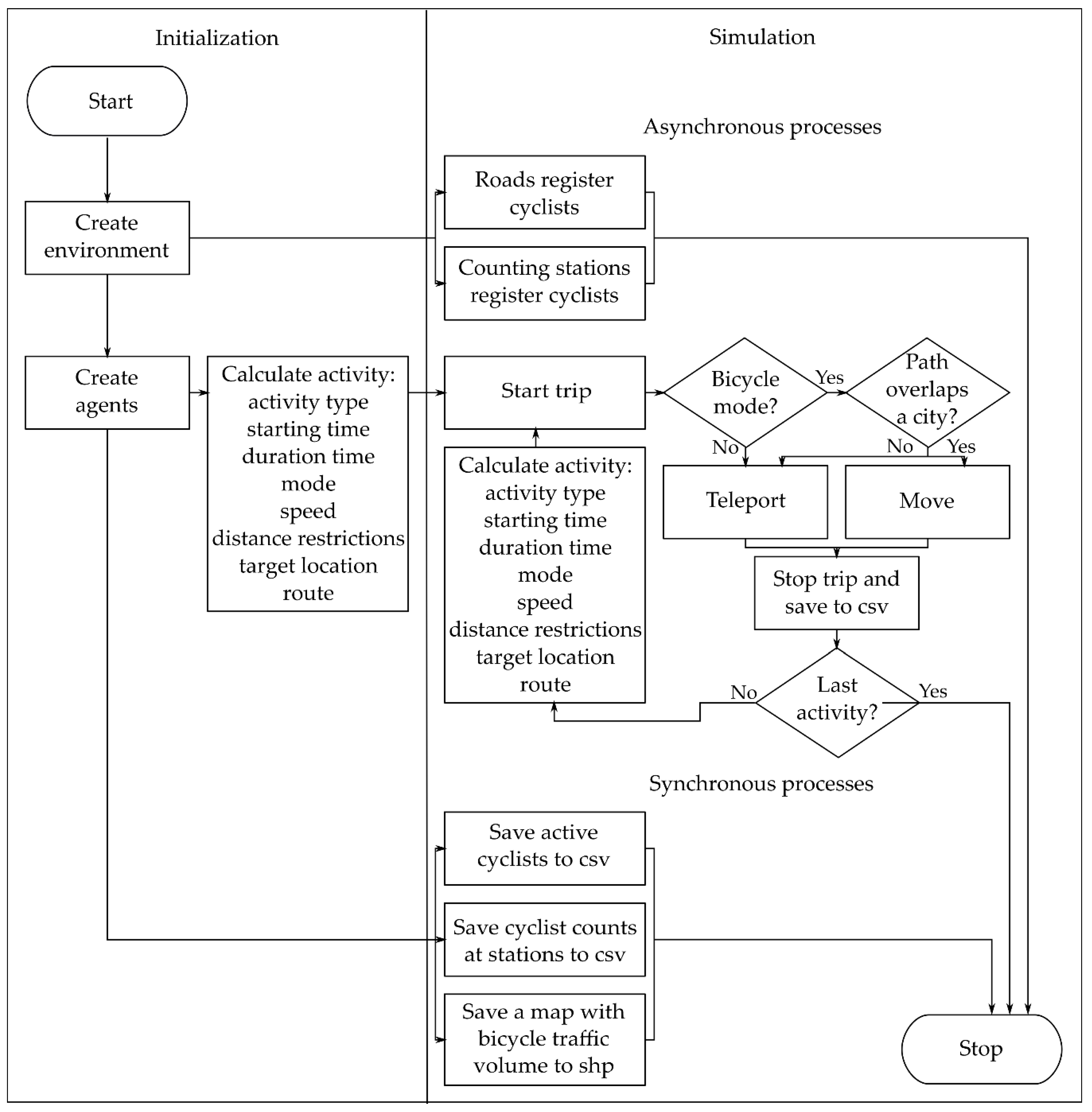
Figure 2 illustrates the key processes that are reenacted in the model every cycle or when conditions are met. Throughout the simulation, persons act asynchronously. They iteratively choose and accomplish desired activities by traveling to facilities by different transportation modes. A person does not have an initial activity chain for the whole day but complements it by assigning a new activity at the end of the current one. The selection of the last activity is integrated as a probability during the activity assignment. Thus, the total amount of activities that a person can undertake depends on the derivatives from the mobility survey. The maximum is eight activities per day.
During the process of activity assignment, behavioral rules determine several activity attributes, such as type, starting time, duration, mode, distance restrictions, speed, and target location. A rule is represented in the form of a probability distribution and characterizes the likelihood of a particular option to be selected. After activity selection, only cyclists that cross a city area travel along a network and register themselves at traversed counting stations and roads. The rest of the persons transfer themselves directly to their destinations, due to the model’s focus is on a bicycle traffic pattern. At the end of each trip, trip-related data, such as synthetic trajectory, distance, travel time, etc., are saved in the “trips” dataset.
Three synchronous processes collect data about traveling cyclists at user-defined time intervals. The “active cyclists” dataset stores the aggregate totals of cyclists traveling around a simulated world according to their trip purposes. Counting stations and a network register the amounts of traversing cyclists into datasets named “counting data” and “traffic volume heatmap”, respectively.

2.1.4. Design Concepts

Several design concepts that define agent-based models were implemented in the bicycle model. The emergence of bicycle traffic flows over space and time is given by the complexity of persons’ diverse mobility behavior, but—at this stage of the model development—not by interactions with each other. Nevertheless, heterogeneity of agents and the probabilistic nature of behavioral rules that govern agents’ decision making make the prediction of traffic volumes emergent. Fitness-seeking behavior is incorporated in the route selection, as persons optimize their paths by safety and distance preferences.
Sensing as the notion of agent awareness of itself and an environment is also implemented in the model. Persons reason about choice options available to them based on the knowledge about their age, gender, and employment. They sense the network quality when navigating to their destinations according to their preferences. Stochasticity is present in the distribution of a population by demographic attributes. Moreover, the modeled rules of activity assignment are based on probability distributions adding the uncertainty of human behavior.
Observation includes monitoring and storing model output for testing and analysis. Active cyclists, traversed cyclists at counting stations, and a network are monitored for verification and validation purposes. For model analysis, trips’ information and roads’ bicycle volumes were collected.

2.1.5. Initialization

During the initialization, the model creates a world with persons and a built environment. The spatial distribution of persons by age, gender, and employment status is calculated from real-world estimates in residential data. For example, if a grid cell has a registered number of female residents aged between 20 and 24, the model will create that number of female persons and assign age randomly within that range.
The model requires a topologically correct network of links for routing operations. Thus, simulated roads connect to a coherent bidirectional network with one-way roads, two-way roads, and restrictions. The network is weighted with a safety index to provide safety-oriented cycling. The adopted calculation of an index follows the indicator-based assessment [35]. Several road indicators are incorporated into the safety index calculation. These are road category, presence of bicycle infrastructure and established cycling routes, vehicle restrictions, gradient, pavement, and maximum motorized speed from the network shapefile.
Counting stations and network intersections are also initialized directly from shapefiles with no additional computation. Next, the model imports probabilities of activity types, modes, and starting and duration times from comma-separated values (CSV) files. Before the simulation day starts, persons are distributed to the initial activity locations.

2.1.6. Submodels

Activity type choice. There are several activity options: staying at home, working, shopping, recreation activity, business-related activity, visiting authorities, visiting doctor, accompanying people, and staying at other places. The probabilities of these options are different for every individual; firstly, because they vary depending on the position of activity in an activity chain (0–7). In Table 1, every column represents the probability distribution of activity types based on the numerical order of a calculated next activity, i.e., activity position. Secondly, an individual’s employment status restricts activity options. For example, a pupil below a certain age can travel to school but cannot go to work. At the beginning of a simulation, every person calculates an initial activity by taking a probability distribution where an activity position is null.
Starting and duration time choices. The process of activity assignment continues with the selection of temporal characteristics. The probability of every activity’s starting time depends on the activity’s type and position in an activity chain. Table A1 in Appendix A shows an example of probabilities for work activity. Throughout a simulated day, passed hours are eliminated from the probability distributions. There are simplified assumptions for school and university activities. Departure time for school is calculated between 7:00 and 8:00, for university, between 8:00 and 18:00. Furthermore, activity types are restricted to possible durations a person can spend at an activity location. In the case of work activity, the duration varies by gender. Moreover, pupils stay at school depending on age. Additional information about duration values can be found in Appendix A (Table A2, Table A3 and Table A4).
Mode choice. There are six available modes, such as walking, bicycle, car, car passenger, public transport, and other transport (Table 2). For the sake of simplification, we assume that a person can only change their mode of transportation at home. The probability distributions of modes vary for every activity type. Moreover, there is a difference between modal splits for region-based and city-based trips.
Distance and speed choice. Another assumption is that modes have different travel distance capacities and speeds. There is a 71% chance a walking trip is shorter than 1 km, and a 29% chance it is between 1 to 5 km. Similar probabilities are given to bicycle trips: distance restrictions can be up to 2 km and 2–8 km with probabilities of 73 and 27%, respectively. Other modes are not restricted by distances. Speed also varies by mode. Walking speed is in the range of 0.7–2.0 m/s, bicycle speed is given 1.6–5.5 m/s. Car, car passenger, and public transport all travel 4.9–14.9 m/s. Other undefined transport has a speed of 2.4–13.6 m/s.
Target choice. A person selects a target location from an available number of relevant facilities that fulfill distance restrictions. The calculation of a suitable workplace has an additional constraint. It takes into account the number of employees every workplace is characterized by. Throughout an activity assignment, a person might not select any activity type or starting time. In such a case, a person returns home and does not travel anymore.
Route choice. The safest and shortest routing options characterize the movement of cyclists and non-cyclists, respectively. The safest routes are calculated using the Dijkstra algorithm and the safety index as impedance. For the shortest routes, the same algorithm uses distance as impedance.
Move. Cyclists whose routes overlap a city area start traveling at calculated departure times along a network toward destinations. The movements are performed according to routing preferences and speed values calculated in prior steps. Non-cyclists and cyclists with trips outside a city do not physically move through a simulated space. They teleport directly to their destinations, and travel times are calculated to represent the real time they would spend on traveling.

2.2. Data

In the proposed agent-based model, we make use of extensive geospatial data sets to define the population, environment, and decision-making rules. Several datasets in Table 3 were acquired to parameterize the bicycle model. The residential data from Statistik Austria [36] provides the basis for modeling the socio-demographic heterogeneity of the underlying population. The data of residency by age, gender, and employment status consists of grid cells with a spatial resolution of 250 m.
The mobility survey data of the province of Salzburg [37] defines behavioral rules. Around 40,000 respondents from the province reported their daily trips. The trips of respondents are ordered in activity chains. Every trip includes attributive information, such as activity ID (sequential number of activity in an activity chain), activity type, timing, distance, and transport mode. The derived distributions of trips by each attribute form probabilistic rules concerning activity types, starting times, modes, distances to a target, and speeds. Furthermore, every simulated activity is characterized by duration time. The corresponding probabilities are inferred from the guidelines and reports of research institutions [38,39,40]. All probability distributions are assembled into separate CSV files for use by the simulation model.
The built environment is represented in the model by an authoritative road network graph [41] and points of interest (POI) from Open Street Map and authoritative sources [42,43,44,45,46]. The workplace facilities are defined by the workplace census information provided by Statistik Austria [47], where employment values are represented as the number of employees per 100 m grid cell. The city’s and region’s outlines are gathered from the official dataset of administrative boundaries in Austria [48]. Lastly, the dataset with existing locations of counting sites in Salzburg [49,50,51] is used to create counting stations in the model.

2.3. Design of Experiments

Given the stochastic nature of probability distributions incorporated in the decision making of agents, a model’s response may vary and include an experimental error [52]. It is recommended to run one simulation several times to achieve meaningful results. The required number of runs is distinct to every model. In order to obtain it, the mean and variability of response values for an increasing number of runs are calculated and analyzed. A response variable can be any record of the model’s non-deterministic output. Lorscheid et al. [52] propose to use the coefficient of variation as an accuracy measure of the mean and standard deviation. To define it, the standard deviation is divided by the mean value. The coefficients of variation fluctuate according to the number of runs until they stabilize, meaning that additional runs do not minimize an error considerably.
In our model, the average execution time of one simulation run is around 40 min. Such an amount of time impedes a 1000-times repetition. A much higher repetition of simulations would be extremely time consuming and just lead to pseudo-accuracy, given the structural model uncertainty due to assumptions. We, thus, consider one simulation run sufficient for the purpose of the model if experimental errors for low simulation runs stay small.
We carry out an analysis to check the variability of errors in model results depending on the increasing number of runs. Restricted by the cost-benefit factor, we limit the maximum number of simulation runs to 10. We choose the daily bicycle volume as a response variable and record it at 20 random locations. At every step, we raise the number of simulation runs and calculate the mean of daily bicycle volumes at single locations as well as the coefficient of variation. The variability of coefficients, such as standard deviation, can then show how the number of additional runs changes the variation in response variables.

2.4. Verification and Validation

Following the common practice in ABM research, the modeling process consists of designing a conceptual model proceeded by formalizing it into an executable program. Wilensky and Rand [23] emphasize the principle of ABM design to progressively implement agents and rules in a model. Thus, at every step of additional complexity, we check if it improves the model according to its stated purpose. This process is coined with monitoring state variables to verify that the model is built correctly. The verification testing is done by displaying the dynamic content of a simulation output on charts and a map within the platform interface. A map displaying the entire environment and moving agents is used to demonstrate that all components of a transportation system are present and responsive as expected. To verify that agents move, some graphs demonstrate temporal distributions of traveling cyclists.
Patterns observed in a real system can facilitate the design and validation of its simplified representation. They often express the structure and underlying processes. The pattern-oriented modeling (POM) framework suggests using patterns to define a model in terms of its components and processes, test its internal organization, and validate results [53]. We use multiple patterns, such as spatial and temporal distributions of cyclists over the study area and their relative frequencies from observed datasets, to indicate the validity of model output.
For the validation, we consider conceptual and operational validities [54]. Conceptual validity tests cause–effect relationships of underlying model concepts using scenario analysis. This step is similar to the POM’s strategy to test how well the alternative theories of decision-making processes reproduce some patterns [53]. We formulate four alternative scenarios (Table 4) to test the impact of the behavioral concepts in our model (behaviorally realistic reference scenario) against the respective null models: activity type choice, target location choice, and starting time choice are tested against random selections, and multi-criteria route choice is tested against the shortest path calculation as its null model.
The comparison of the scenarios is done by investigating the operational validities of their results. Operational validity checks whether the bicycle model and four alternative scenarios are acceptable for the intended purpose. It examines how well model results imitate observed data. According to Kang and Aldstadt [55], validating the output of a spatially explicit model at different spatio-temporal scales increases its reliability. Such validation eliminates the risk of faulty generative mechanisms when a model reproduces patterns either on a macro scale or a micro scale.
Validation data were acquired from the stationary and mobile sensors that captured the movements of cyclists in the region during October–November. The patterns derived from the data serve as validation criteria at different spatial and temporal scales. The acquired counting data represent counts of cyclists at nine stations between 2012 and 2019 [49,50,51]. The minimum temporal granularity is 15 min. The first criterion is the total amount of traversed cyclists at counting stations over a day. The selected pattern is at a spatially local and temporarily long-term scale. The mean absolute error is used as a comparison method. The absolute error is the difference between simulated and observed daily counts at one station. The average of absolute errors at all stations comprises the mean absolute error. This measure of error demonstrates the magnitude of inaccuracy in model results. The second criterion at a spatially local and temporarily short-term scale is the hourly number of traversed cyclists at counting stations throughout the day. Pearson’s correlation analysis is used to show the strength of the association between observed and simulated hourly values.
The two mobile applications that collected spatio-temporal bicycling data are Bike Citizens and Strava [56,57]. Both datasets were spatially matched to the network used in the model. The derived daily totals of traffic volumes per network link are the third validation criterion. The pattern is at spatially local and temporarily long-term scale. Again, Pearson’s correlation analysis is employed.
Finally, validation examines the patterns of relative frequencies in the observed and simulated bicycle traffic at counting stations. Mobility can be influenced by the spatial distribution of attractions and the landscape of a city. Therefore, we inspect the ratio of cyclists between two sides of the city divided by the river Salzach. The next pattern is the ratio of cyclists traversing stations in the city center vs. on the outskirts. At last, we use the morning and afternoon peak ratio to validate bicycle traffic at stations.

3. Results

The model simulated the mobility of around 186,000 persons in the extended region of Salzburg city for one day. Simulated counting stations gathered information about how many cyclists traversed them every hour. The temporal distributions of cyclists and their means are shown in Figure 3 for comparison with the observed data from actual counting stations. The model at the majority of stations captures two distinct peaks of busiest traffic per day. The ratios of cyclists at the morning and afternoon peaks are similar to the observed ratios (Table 5). The variation between stations according to their spatial locations also fits the observed data. Peripheral stations, such as Ischlerbahnstraße and Moosbrücker Weg, have the lowest observed and simulated daily counts, whereas central Rudolfskai and Giselakai stations have the highest. The simulated daily counts at central stations vs. peripheral stations result in a valid ratio of 0.71:0.29 with respect to the observed ratio of 0.85:0.15.
Figure 4a shows the spatial distribution of bicycle traffic flows on the network. It demonstrates heavily used bicycle corridors, such as the one that emerges along the river Salzach. This corridor attracts most cyclists, because it connects northern and southern parts of the city, providing bicycle infrastructure separated from motorized traffic. Minimum obstacles, such as traffic lights and junctions, also characterize the corridor. Several arteries that gather at the Salzach corridor connect the east and west of the city. They represent the evidence of daily relocations of residents between the city halves split by the river. The ratio of registered cyclists at stations on the west side vs. east side is 0.49:0.51, which corresponds well to the observed ratio of 0.53:0.47.
Due to the model’s stochasticity, it is important to check the uncertainty of results depending on the number of simulation runs. Experimental errors are represented as the coefficients of variations in bicycle traffic volumes at 20 random stations. In Figure 5, the variability of coefficients derived from different number of runs is demonstrated as coefficients’ mean, standard deviations, and minimum and maximum values. The majority of coefficients indicate small variabilities in response values. Few locations have null coefficients because of the recorded null bicycle traffic volumes in all of the simulation runs. The standard deviations of coefficients lean towards 0.0 in most of the locations. This means that the different numbers of runs at the low range produce similar results. These outcomes justify that one simulation run is sufficient for using the model.
The scenario analysis compares the model (behaviorally realistic reference model) with four alternative scenarios to demonstrate the significance of implemented model concepts. Figure 4b–e show traffic volumes resulting in alternative scenarios. The pattern is more emphasized in the random activity type choice and unrestricted target location choice scenarios, as there are more trips simulated. The random starting time choice scenario shows less traffic on the network. Lastly, there is a spatially different pattern emerging in the shortest path route choice scenario.
The concepts of activity type choice and target location choice affect activity locations and the total number of trips carried out by individuals. In turn, the first validation criterion, which is daily counts at stations, is responsive to changes in the distribution of activities. Thus, it can best demonstrate the soundness of these two concepts. Figure 6 illustrates the observed and simulated daily numbers of passing cyclists at each counting station for every scenario. In the reference scenario, the mean absolute error of simulated daily counts compared to observed counts are 1002.07 cyclists on average. In the random activity type choice scenario, the random assignment of activity types changes the spatial and temporal distribution of attractive locations. The error increases by 71.04% to 1713.9 cyclists. A greater increase of 255.12% is observed in the unrestricted target location choice scenario. The error is 3257.9 cyclists. According to scenario rules, persons are unrestricted in the selection of destinations in regards to distances. Hence, bicycle trips can be 500 m or as long as 20 km long.
The next model concept is the starting time choice responsible for the temporal distribution of trips. Its validity is checked by the second validation criterion, i.e., the hourly distribution of cyclists at counting stations. The results of the correlation analyses between simulated and observed data for each scenario are listed in Table 6. In the reference (behaviorally realistic) scenario, the correlation coefficients range between 0.60 and 0.89, showing very significant relationships with p < 0.001 at all stations. Persons in the random starting time choice scenario travel at random times of a day causing insignificant relationships. Its correlation coefficients range between 0.09 and 0.35, which are much lower than in the reference scenario.
Maps in Figure 5 show how the concept of route choice, in particular, affects the spatial distribution of cyclists over the network. Thus, we compare the daily traffic volumes over a network with the observed data to justify the concept of route choice in Table 7. Moderate and weak correlations are observed in the reference (behaviorally realistic) scenario. The coefficients are 0.64 and 0.43 with p < 0.001 for Bike Citizens and Strava datasets, respectively. In the shortest path route choice scenario, shortest paths are preferred over safest paths during navigation. The coefficients are 0.35 and 0.14 with p < 0.001. There is a weak positive correlation with the Bike Citizens dataset and absolutely no correlation with the Strava dataset.

4. Discussion and Conclusions

In our research, we simulated bicycle traffic flows as a phenomenon emerging from individual mobility behavior. Such simulation of emergent traffic flows integrates the strengths of two strains of research. First, there are the behaviorally realistic bicycle models that have mainly focused on emergent phenomena at local scale levels [13,14]. Second, there is the traffic-flow modeling at a regional level that has, thus far, mainly been based on aggregated data [15].
The part of the experiment’s design is the assessment of uncertainty in results caused by the model’s stochasticity in decision making. The evaluated experimental errors of results are small and do not strongly vary depending on the number of simulation runs. Given the low coefficient of variation, the model produces results of sufficient accuracy with one simulation run.
Through scenario analysis, we could demonstrate that models with demographically parametrized behavior outperform stochastic null models. We conclude that dynamic activity assignment allows for the inclusion of uncertainty of human behavior as opposed to the appointment of pre-defined activity chains. Although, the strong trends in activity chains are still preserved in probabilistic rules. The sequential number of the next activity is a significant factor in determining its type and start time. Its consideration allows the majority of an active population to start their day with long-term utilitarian activities in the mornings, leaving other activities for the rest of a day. The inclusion of distance limitations for cyclists and pedestrians prevents non-city residents from taking longer trips across a city in a simulation. It confirms the fact that persons tend to choose closer facilities, especially when walking or bicycling. Lastly, the safest routing for cycling better corresponds to the observed data than the shortest routing.
While scenario analysis justified the model’s complexity, the empirical validation showed different, significant relationships between simulated and observed data: strong relationships in terms of temporal patterns and moderate to weak relationships in terms of the spatial distribution of flows, depending on the reference dataset. We are aware of the model’s inaccuracies in its results. However, considering the quality of currently available input and validation data, the model presented in this paper is a step forward in terms of methodology (ABM for macroscopic simulation of bicycle flows) and predictive power. Moreover, the validation of the relative frequencies in bicycle patterns upholds the strength of the model’s internal design. The cycling ratios of morning vs. afternoon peaks, city center vs. outskirts, and west vs. east sides of the city were imitated well in comparison to the observed patterns.
The model is based on a coherent travel theory with a complete set of individual choices. Thus, it simulates the mobility of cyclists that can address planned policy strategies and changes in urban infrastructure. Bicycle traffic flows is an emergent phenomenon that results from mobility. In contrast, widely used traditional four-step models lack such a behavioral background and calculate traffic flows solely based on aggregated assignments of trips. They represent a static modeling system that cannot express individual decisions and connect the characteristics and preferences of travelers with their trips [16].
Including individual preferences leads us from models that are “just” phenomenologically correct to behaviorally realistic simulations. The grand advantage of behaviorally realistic models is that they can adapt to city planning scenarios, and they, thus, provide city planners with a powerful toolset to design holistic concepts for cycling mobility. Questions such as “how will bicycle traffic patterns change, if we build a new company with 1000 new employees at location xy” or “what if we add a bicycle lane to road x” or “where to place bike-sharing stations” can only be answered with a behaviorally realistic model.
Although behavioral realism could improve the model, there are still deviations from real bicycle traffic. The model explains general patterns well but needs further improvement to answer more specific questions. Despite the strongly correlated temporal distributions of cyclists, the problem with the magnitudes of error persists. Considering the ultimate safety preference in routing can be a fallacy. In contrast to the implemented routing, Leao and Pettit [29], in their study, determined that around 80% of recorded GPS tracks of cycling commuters matched a synthesized sample of shortest path trips. The fact that commuting trips are more sensitive to distance is also evident in the study by Broach et al. [58]. Thus, the assumption of the shortest path preference for commuting trips is a potential model improvement.
Furthermore, in the real world, a bicycle path might not always be the optimal option from a safety and distance point of view. This unusual behavior can be an example of unique cognitive processes in human behavior that an agent-based model is not able to capture [59]. The model would benefit from the consideration of traffic lights in routing decisions, since cyclists tend to choose less disturbed paths [60].
There are also deficiencies in the quality of available input and validation data. Currently, travel decisions depend on derivatives from the regional mobility survey. The main concern with such regional surveys is the risk of incompleteness, the biased representation of a population, or the lack of necessary information. For example, the workplace census data has its limits for modeling workplace facilities. The selection of workplace destinations depends on the number of employees at locations of their official registration and not where they actually work. This is a possible cause of observed spatial misbalance of simulated traffic between the eastern and western parts of the city
The incomplete representativeness of crowd-sourced mobility data may attribute to some discrepancies in validation results [61,62]. Data collection by mobile applications used in this study depends on user participation. Users are often health-oriented people interested in recording bicycle trips. Thus, data could omit utilitarian trips to work, schools, and universities by other groups of people. Moreover, the number of trips recorded by the two applications is small (taken trajectories from both applications together, 0.17% of the average daily number of cyclists registered by Rudolfskai counting station) and, thus, of limited representativeness.
Apart from specific data quality, a problem arises from the fact that demographic parameterization of mobility behavior is generally data hungry. Thus, transferability may be limited. The remaining question is: how robust is the model if transferred to other regions? Which components are to be re-parameterized with local data; what are generalizable parameters that can be transferred? If transferability is provided for the key components, “data hungriness” is less problematic.
The results highlight the added value of using transport ABMs at a regional level, where spatio-temporal traffic patterns emerge from the individual behavior of residents. The output data helps to distinguish the usability of existing and potential bicycle paths necessary for planning strategies and investments. Although only bicycle movement is simulated, the simulation of mode choice includes all major transportation modes. This facilitates the potential integration of additional concepts to capture travel patterns of other transportation modes. Moreover, the model can facilitate the investigation of other urban dynamic processes as an integrated transport module.

Author Contributions

Conceptualization, Dana Kaziyeva, Martin Loidl, and Gudrun Wallentin; data curation, Dana Kaziyeva; formal analysis, Dana Kaziyeva; funding acquisition, Martin Loidl; investigation, Dana Kaziyeva; methodology, Dana Kaziyeva, Martin Loidl, and Gudrun Wallentin; project administration, Martin Loidl; resources, Dana Kaziyeva, Martin Loidl, and Gudrun Wallentin; software, Dana Kaziyeva; supervision, Martin Loidl and Gudrun Wallentin; validation, Dana Kaziyeva; visualization, Dana Kaziyeva; writing—original draft, Dana Kaziyeva; writing—review and editing, Dana Kaziyeva, Martin Loidl, and Gudrun Wallentin. All authors have read and agreed to the published version of the manuscript.

Funding

This research was funded by Austrian Research Promotion Agency through the FamoS project, grant number 855034; and by the Austrian Science Fund through the Doctoral College GIScience at the University of Salzburg, grant number DK W 1237-N23.

Institutional Review Board Statement

Not applicable.

Informed Consent Statement

Not applicable.

Data Availability Statement

Publicly available datasets were analyzed in this study. This data can be found together with the model code here: https://www.comses.net/codebase-release/897ca5d7-a00e-4515-8e14-9fc015ea183e/ (accessed on 19 February 2021).

Acknowledgments

Open Access Funding by the Austrian Science Fund (FWF). The authors would also like to thank Bike Citizens for providing trajectory data from their mobile application (https://www.bikecitizens.net/app/ (accessed on 19 February 2021)), Strava Metro for providing aggregated and de-identified trajectory data (https://www.strava.com/mobile (accessed on 19 February 2021)), and the City Administration of Salzburg for providing counts data.

Conflicts of Interest

The authors declare no conflict of interest.

Appendix A

Table A1. Probability distributions of departure hours to work (%) by activity position in an activity chain.
Hour1234567
10.321.260.550.520.970.000.00
20.080.000.050.000.000.000.00
30.120.180.000.000.000.000.00
40.510.090.000.000.000.000.00
51.810.180.050.000.000.000.00
610.112.960.250.000.000.000.00
734.2112.662.201.050.000.000.00
836.7532.325.015.761.950.000.00
99.9215.804.712.620.970.000.00
102.148.443.661.832.602.831.72
111.005.124.866.543.252.831.72
120.564.134.916.816.495.663.45
130.674.6727.9118.3213.645.6613.79
140.773.7721.8418.8519.4816.9810.34
150.291.978.479.6914.949.4310.34
160.191.354.116.8110.0615.0915.52
170.101.714.918.9010.0620.7513.79
180.121.263.315.245.529.4312.07
190.090.812.253.663.906.6010.34
200.100.450.301.052.273.775.17
210.020.090.250.790.970.001.72
220.070.810.251.571.620.000.00
230.030.000.000.000.970.940.00
240.010.000.150.000.320.000.00
Table A2. Durations by activity type.
Activity TypeDuration, hClosing Time
Home0.5–1-
Other place0.25–323:00
Business0.25–318:00
University2–620:00
Shop0.25–318:00
Authority0.518:00
Doctor118:00
Recreation1–323:00
Bringing0.25–118:00
Table A3. Probability distributions of work durations by gender.
Duration, hFemaleMale
0–2.27.83
2.4–4.819.23.3
5–722.43.9
7.2–840.361.3
8.2–11.89.425.2
12–170.83
0–170.10.3
Table A4. School durations by age.
AgeDuration, hClosing Time
6–7616:00
8–9716:00
10–13816:00
Over 156–816:00

References

  1. BMLFUW. Cycling Masterplan 2015–2025; Federal Ministry of Agriculture, Forestry, Environment and Water Management: Vienna, Austria, 2015.
  2. ECF. EU Cycling Strategy: Recommendations for Delivering Green Growth and an Effective Mobility in 2030; European Cyclists’ Federation: Brussels, Belgium, 2017. [Google Scholar]
  3. Mertens, L.; Compernolle, S.; Deforche, B.; MacKenbach, J.D.; Lakerveld, J.; Brug, J.; Roda, C.; Feuillet, T.; Oppert, J.-M.; Glonti, K.; et al. Built environmental correlates of cycling for transport across Europe. Health Place 2017, 44, 35–42. [Google Scholar] [CrossRef] [Green Version]
  4. Pucher, J.; Dill, J.; Handy, S. Infrastructure, programs, and policies to increase bicycling: An international review. Prev. Med. 2010, 50, S106–S125. [Google Scholar] [CrossRef] [PubMed]
  5. Sallis, J.F.; Cerin, E.; Conway, T.L.; Adams, M.A.; Frank, L.D.; Pratt, M.; Salvo, D.; Schipperijn, J.; Smith, G.; Cain, K.L.; et al. Physical activity in relation to urban environments in 14 cities worldwide: A cross-sectional study. Lancet 2016, 387, 2207–2217. [Google Scholar] [CrossRef] [Green Version]
  6. Handy, S.L.; Van Wee, B.; Kroesen, M. Promoting Cycling for Transport: Research Needs and Challenges. Transp. Rev. 2014, 34, 4–24. [Google Scholar] [CrossRef]
  7. Loidl, M.; Stutz, P.; Fernandez La Puente de Battre, M.D.; Schmied, C.; Reich, B.; Bohm, P.; Sedlacek, N.; Niebauer, J.; Niederseer, D. Merging self-reported with technically sensed data for tracking mobility behaviour in a naturalistic in-tervention study. Insights from the GISMO study. Scand. J. Med. Sci. Sports 2020. [Google Scholar] [CrossRef] [Green Version]
  8. Shen, L.; Stopher, P.R. Review of GPS Travel Survey and GPS Data-Processing Methods. Transp. Rev. 2014, 34, 316–334. [Google Scholar] [CrossRef]
  9. Batty, M. A Generic Framework for Computational Spatial Modelling. In Agent-Based Models of Geographical Systems; Heppenstall, A.J., Crooks, A.T., See, L.M., Batty, M., Eds.; Springer Netherlands: Dordrecht, The Netherlands, 2012; pp. 19–50. [Google Scholar]
  10. Ortúzar Salar, J.d.D.; Willumsen, L.G. Modelling Transport, 4th ed.; John Wiley & Sons: Chichester, UK, 2011. [Google Scholar]
  11. Aziz, H.A.; Park, B.H.; Morton, A.; Stewart, R.N.; Hilliard, M.; Maness, M. A high resolution agent-based model to support walk-bicycle infrastructure investment decisions: A case study with New York City. Transp. Res. Part C Emerg. Technol. 2018, 86, 280–299. [Google Scholar] [CrossRef]
  12. Rybarczyk, G. Simulating bicycle wayfinding mechanisms in an urban environment. Urban Plan. Transp. Res. 2014, 2, 89–104. [Google Scholar] [CrossRef] [Green Version]
  13. Agarwal, A.; Zilske, M.; Rao, K.R.; Nagel, K. An Elegant and Computationally Efficient Approach for Heterogeneous Traffic Modelling Using Agent Based Simulation. Procedia Comput. Sci. 2015, 52, 962–967. [Google Scholar] [CrossRef] [Green Version]
  14. Shan, X.; Li, Z.; Chen, X.; Ye, J. A Modified Cellular Automaton Approach for Mixed Bicycle Traffic Flow Modeling. Discret. Dyn. Nat. Soc. 2015, 2015, 1–11. [Google Scholar] [CrossRef] [Green Version]
  15. Jacyna, M.; Wasiak, M.; Kłodawski, M.; Gołębiowski, P. Modelling of Bicycle Traffic in the Cities Using VISUM. Procedia Eng. 2017, 187, 435–441. [Google Scholar] [CrossRef]
  16. Transportation Research Board. Metropolitan Travel Forecasting: Current Practice and Future Direction-Special Report 288; The National Academies Press: Washington, DC, USA, 2007; p. 144. [Google Scholar] [CrossRef]
  17. Fagnant, D.J.; Kockelman, K. A direct-demand model for bicycle counts: The impacts of level of service and other factors. Environ. Plan. B Plan. Des. 2015, 43, 93–107. [Google Scholar] [CrossRef] [Green Version]
  18. Hankey, S.; Lindsey, G.; Wang, X.; Borah, J.; Hoff, K.; Utecht, B.; Xu, Z. Estimating use of non-motorized infrastructure: Models of bicycle and pedestrian traffic in Minneapolis, MN. Landsc. Urban Plan. 2012, 107, 307–316. [Google Scholar] [CrossRef]
  19. Lu, T.; Mondschein, A.; Buehler, R.; Hankey, S. Adding temporal information to direct-demand models: Hourly estimation of bicycle and pedestrian traffic in Blacksburg, VA. Transp. Res. Part D Transp. Environ. 2018, 63, 244–260. [Google Scholar] [CrossRef]
  20. Cooper, C.H. Using spatial network analysis to model pedal cycle flows, risk and mode choice. J. Transp. Geogr. 2017, 58, 157–165. [Google Scholar] [CrossRef]
  21. McDaniel, S.; Lowry, M.B.; Dixon, M. Using Origin–Destination Centrality to Estimate Directional Bicycle Volumes. Transp. Res. Rec. J. Transp. Res. Board 2014, 2430, 12–19. [Google Scholar] [CrossRef]
  22. Loidl, M.; Werner, C.; Heym, L.; Kofler, P.; Innerebner, G. Lifestyles and Cycling Behavior—Data from a Cross-Sectional Study. Data 2019, 4, 140. [Google Scholar] [CrossRef] [Green Version]
  23. Wilensky, U.; Rand, W. An Introduction to Agent-Based Modeling: Modeling Natural, Social, and Engineered Complex Systems with NetLogo; MIT Press: Cambridge, MA, USA, 2015. [Google Scholar]
  24. Axelrod, R. Advancing the art of simulation in the social sciences. Complexity 1997, 3, 16–22. [Google Scholar] [CrossRef] [Green Version]
  25. Loidl, M.; Wallentin, G.; Cyganski, R.; Graser, A.; Scholz, J.; Haslauer, E. GIS and Transport Modeling—Strengthening the Spatial Perspective. ISPRS Int. J. Geo-Inf. 2016, 5, 84. [Google Scholar] [CrossRef] [Green Version]
  26. Miller, H.J.; Shaw, S.-L. Geographic Information Systems for Transportation in the 21st Century. Geogr. Compass 2015, 9, 180–189. [Google Scholar] [CrossRef]
  27. Crooks, A.T.; Castle, C.J.E. The Integration of Agent-Based Modelling and Geographical Information for Geospatial Simulation. In Agent-Based Models of Geographical Systems; Heppenstall, A.J., Crooks, A.T., See, L.M., Batty, M., Eds.; Springer: Dordrecht, The Netherlands, 2012; pp. 219–251. [Google Scholar]
  28. Wallentin, G.; Loidl, M. Agent-based Bicycle Traffic Model for Salzburg City. GI_Forum J. Geogr. Inf. Sci. 2015, 1, 558–566. [Google Scholar] [CrossRef]
  29. Leao, S.Z.; Pettit, C. Mapping Bicycling Patterns with an Agent-Based Model, Census and Crowdsourced Data. In Agent Based Modelling of Urban Systems. ABMUS 2016. Lecture Notes in Computer Science; Namazi-Rad, M.R., Padgham, L., Perez, P., Nagel, K., Bazzan, A., Eds.; Springer: Cham, Switzerland, 2017; pp. 112–128. [Google Scholar] [CrossRef]
  30. Ziemke, D.; Metzler, S.; Nagel, K. Modeling bicycle traffic in an agent-based transport simulation. Procedia Comput. Sci. 2017, 109, 923–928. [Google Scholar] [CrossRef]
  31. Veldhuis, L.O. Applications of Agent Based Modelling: Analysis and Simulation of Bicycle Traffic in Urban Environments; Report; Wageningen University: Wageningen, The Netherlands, 2018. [Google Scholar]
  32. Taillandier, P.; Gaudou, B.; Grignard, A.; Huynh, Q.-N.; Marilleau, N.; Caillou, P.; Philippon, D.; Drogoul, A. Building, composing and experimenting complex spatial models with the GAMA platform. GeoInformatica 2019, 23, 299–322. [Google Scholar] [CrossRef] [Green Version]
  33. Kaziyeva, D.; Wallentin, G.; Loidl, M. Bicycle Model, 2.0.0; CoMSES Computation Model Library. Available online: https://www.comses.net/codebase-release/897ca5d7-a00e-4515-8e14-9fc015ea183e/ (accessed on 1 December 2020).
  34. Grimm, V.; Berger, U.; Bastiansen, F.; Eliassen, S.; Ginot, V.; Giske, J.; Goss-Custard, J.; Grand, T.; Heinz, S.K.; Huse, G.; et al. A standard protocol for describing individual-based and agent-based models. Ecol. Model. 2006, 198, 115–126. [Google Scholar] [CrossRef]
  35. Loidl, M.; Zagel, B. Assessing Bicycle Safety in Multiple Networks with Different Data Models. In Proceedings of the GI_Forum 2014—Geospatial Innovation for Society, Salzburg, Austria, 1–4 July 2014; Osterreichische Akademie der Wissenschaften: Vienna, Austria; Berlin, Germany; Offenbach, Germany, 2015; Volume 2014, pp. 144–154. [Google Scholar]
  36. Federal Statistics Austria. Registerzählung 2011; STATISTIK AUSTRIA: Vienna, Austria, 2011. [Google Scholar]
  37. Federal State of Salzburg—Transport Department. Mobilitätserhebung Land Salzburg; Land Salzburg—Straßenbau und Verkehrsplanung: Salzburg, Austria, 2012.
  38. Austrian Institute of Economic Research. Verteilung der Arbeitszeit WIFO-Beitrag zum Sozialbericht 2015–2016. Available online: http://www.wifo.ac.at/jart/prj3/wifo/resources/person_dokument/person_dokument.jart?publikationsid=59268&mime_type=application/pdf (accessed on 11 January 2018).
  39. Paris Lodron University of Salzburg. Mitteilungsblatt—Sondernummer der Paris Lodron-Universität Salzburg. Available online: https://online.uni-salzburg.at/plus_online/wbMitteilungsblaetter.displayHTML?pNr=46397&pQuery= (accessed on 11 January 2018).
  40. State Education Authority Salzburg. Richtlinien für Schulleitungen 2006. Available online: http://www.za.gierzinger.com/aktuell_files/2010-09-21_schulzeiterlass-LSR_2006_vers3.pdf (accessed on 11 January 2018).
  41. ASFINAG; ITS Vienna Region; Land Burgenland; Land Kärnten; Land Niederösterreich; Land Oberösterreich; Land Salzburg; Land Steiermark; Land Tirol; Land Vorarlberg; et al. Intermodales Verkehrsreferenzsystem Österreich (GIP.at) Österreich. Open Data Österreich. Available online: https://www.data.gv.at/katalog/dataset/3fefc838-791d-4dde-975b-a4131a54e7c5 (accessed on 12 November 2019).
  42. City Administration Salzburg. Open Government Daten der Stadt Salzburg. Stadt Salzburg Web Feature Service OGD. Available online: https://data.stadt-salzburg.at/geodaten/wfs?service=WFS&request=GetFeature&typeNames=ogdsbg:amtsgebaeude (accessed on 2 December 2019).
  43. Federal State of Salzburg—GIS Department. Universitäten Land Salzburg. Open Data Österreich. Available online: https://www.data.gv.at/katalog/dataset/6bcc821d-aef8-4134-aeb5-fdf5993a4dd8 (accessed on 2 December 2019).
  44. Federal State of Salzburg—GIS Department. Ärzte Land Salzburg. Open Data Österreich. Available online: https://www.data.gv.at/katalog/dataset/8bd69af0-d42a-4777-beb6-1e8e87145a23 (accessed on 2 December 2019).
  45. Federal State of Salzburg—IT Department. Verwaltungsadressen—Land Salzburg. Open Data Österreich. Available online: https://www.data.gv.at/katalog/dataset/d49a127d-f60f-4d6f-bb1c-46d70ff14699 (accessed on 20 April 2020).
  46. OpenStreetMap. OSM Dump—Austria. Geofabrik GmbH. Available online: https://download.geofabrik.de/europe/austria.html (accessed on 1 December 2019).
  47. Federal Statistics Austria. Abgestimmte Erwerbsstatistik—Demographie—2013; STATISTIK AUSTRIA: Vienna, Austria, 2013. [Google Scholar]
  48. Bundesamt für Eich- und Vermessungswesen. Verwaltungsgrenzen (VGD)—Stichtagsdaten Grundstücksgenau. Open Data Österreich. Available online: https://www.data.gv.at/katalog/dataset/51bdc6dc-25ae-41de-b8f3-938f9056af62 (accessed on 3 April 2019).
  49. GPV—Günther Pichler GmbH. Radverkehrszählungen Stadt Salzburg. Eco-Counter API. Available online: https://www.eco-visio.net/ (accessed on 23 January 2020).
  50. GPV—Günther Pichler GmbH. Radverkehrszählungen Land Salzburg. Eco-Counter API. Available online: https://www.eco-visio.net/ (accessed on 23 January 2020).
  51. Paris Lodron University of Salzburg—Interfaculty Department Z_GIS. Mobile Radverkehrszählung Z_GIS. Eco-Counter API. Available online: https://www.eco-visio.net/ (accessed on 23 January 2020).
  52. Lorscheid, I.; Heine, B.-O.; Meyer, M. Opening the ‘black box’ of simulations: Increased transparency and effective communication through the systematic design of experiments. Comput. Math. Organ. Theory 2011, 18, 22–62. [Google Scholar] [CrossRef]
  53. Grimm, V.; Revilla, E.; Berger, U.; Jeltsch, F.; Mooij, W.M.; Railsback, S.F.; Thulke, H.-H.; Weiner, J.; Wiegand, T.; DeAn-gelis, D.L. Pattern-Oriented Modeling of Agent-Based Complex Systems: Lessons from Ecology. Science 2005, 310, 987–991. [Google Scholar] [CrossRef] [Green Version]
  54. Rykiel, E.J. Testing ecological models: The meaning of validation. Ecol. Model. 1996, 90, 229–244. [Google Scholar] [CrossRef]
  55. Kang, J.-Y.; Aldstadt, J. Using multiple scale spatio-temporal patterns for validating spatially explicit agent-based models. Int. J. Geogr. Inf. Sci. 2018, 33, 193–213. [Google Scholar] [CrossRef]
  56. Paris Lodron University of Salzburg—Interfaculty Department Z_GIS. Bike Citizens Data. 2019. Available online: https://www.uni-salzburg.at/index.php?id=147&L=1 (accessed on 19 February 2021).
  57. Paris Lodron University of Salzburg—Interfaculty Department Z_GIS. Strava Metro Data. 2020. Available online: https://uni-salzburg.elsevierpure.com/en/activities/gis-in-central-asia-conference-2020 (accessed on 19 February 2021).
  58. Broach, J.; Dill, J.; Gliebe, J. Where do cyclists ride? A route choice model developed with revealed preference GPS data. Transp. Res. Part A Policy Pract. 2012, 46, 1730–1740. [Google Scholar] [CrossRef]
  59. El-Amine, S.; Galland, S.; Yasar, A.-U.-H.; Koukam, A. Demand for Agent-Based Transportation Models & Social Behavioral Challenges. Procedia Comput. Sci. 2017, 113, 210–216. [Google Scholar] [CrossRef]
  60. Van Duppen, J.; Spierings, B. Retracing trajectories: The embodied experience of cycling, urban sensescapes and the commute between ‘neighbourhood’ and ‘city’ in Utrecht, NL. J. Transp. Geogr. 2013, 30, 234–243. [Google Scholar] [CrossRef] [Green Version]
  61. Lissner, S.; Francke, A.; Becker, T. Modeling Cyclists Traffic Volume-Can Bicycle Planning benefit from Smartphone based Data? In Proceedings of the 7th Transport Research Arena TRA 2018, Vienna, Austria, 16–19 April 2018. [Google Scholar]
  62. Watkins, K.; Ammanamanchi, R.; LaMondia, J.; Dantec, C.A.L. Comparison of Smartphone-based Cyclist GPS Data Sources. In Proceedings of the Transportation Research Board 95th Annual Meeting, Washington, DC, USA, 10–14 January 2016. [Google Scholar]
Figure 1. The study area of the greater region of Salzburg city with the transportation network and counting stations.
Ijgi 10 00088 g001
Figure 2. The flowchart of the processes in the bicycle model.
Ijgi 10 00088 g002
Figure 3. The temporal distribution of traversed cyclists at stations by an hour; grey links represent the mean numbers of traverses in simulated results and observed data.
Ijgi 10 00088 g003
Figure 4. Bicycle traffic volumes of one simulation day in scenarios: (a) reference; (b) activity type choice; (c) target location choice; (d) starting time choice; (e) route choice.
Ijgi 10 00088 g004
Figure 5. The box plot of the coefficients of variation of bicycle traffic volumes at random locations depending on the number of simulation runs. Each box represents coefficients’ mean, standard deviations, and maximum and minimum values.
Ijgi 10 00088 g005
Figure 6. The daily totals of traversed cyclists at stations and the average mean absolute errors by scenario.
Ijgi 10 00088 g006
Table 1. Probability distributions of activity types (%) in columns depending on an activity position in an activity chain (0–7).
Activity Position in an Activity Chain
01234567
Home97.440.7770.0313.8158.4918.4647.4425.06
Other place2.566.683.706.603.684.834.443.31
Work0.0040.903.386.272.142.141.631.28
Business0.003.734.173.533.213.033.382.59
Education0.0016.822.221.980.710.560.430.49
Shop0.0016.447.249.164.394.142.871.46
Authority0.000.200.150.100.090.010.020.00
Doctor0.003.470.871.170.410.510.320.13
Recreation0.004.843.079.294.227.354.914.86
Bringing0.005.501.524.013.284.204.023.54
None0.000.643.6644.1019.3754.7730.5657.28
Table 2. Probability distributions of modes (%) by activity type and extent.
WalkBicycleCarCar PassengerPublic TransportOther
City extent
Home25.6322.6228.395.921.8415.60
Other place31.2515.9531.047.441.0613.25
Work21.0625.1037.482.621.6112.14
Business13.0414.9262.372.550.676.45
School29.2617.327.386.986.0433.02
University29.2617.327.386.986.0433.02
Shop34.6616.5832.726.190.489.36
Authority28.139.3831.2518.753.139.38
Doctor18.0517.2933.467.521.8821.80
Recreation27.8718.9029.908.490.8414.00
Bringing16.138.1763.666.880.434.73
Region extent
Home13.488.8155.2310.977.364.16
Other place21.748.1251.5913.222.233.11
Work7.918.0170.485.114.484.01
Business3.752.7583.095.071.993.35
School21.257.5110.7214.8233.1712.53
University21.257.5110.7214.8233.1712.53
Shop18.5210.8057.9210.371.161.23
Authority20.909.7050.7514.183.730.75
Doctor11.645.7058.7917.293.323.26
Recreation22.789.7045.2818.152.091.99
Bringing10.513.7080.284.570.270.68
Table 3. Input data of the bicycle model.
Model ConceptInput Data
Persons’ residency and sociodemographic characteristics
  • Residential data in Salzburg province
Behavioral rules
  • Mobility survey for Salzburg province
  • Social report with working hours of employees in Austria
  • Guidelines for school administrators with duration times in Salzburg Province
  • The European Credit Transfer and Accumulation System (ECTS) guideline at the University of Salzburg with duration times
City and region outline
  • Administrative boundaries in Austria
Network and intersections
  • The intermodal traffic reference system of Austria
Facilities
  • Workplace census data in Salzburg province
  • Locations of doctors, universities, city and federal authorities, schools, shops, recreation, hospitals, kindergartens
Counting stations
  • Locations of counting sites in Salzburg city
Table 4. The alternative scenarios of model concepts with concept descriptions, evaluation criteria, and comparison methods.
Model ConceptReference ScenarioAlternative ScenarioValidation CriteriaComparison Method
Activity type choiceProbability distributionRandom
  • Daily bicycle volume at stations
  • Hourly bicycle volume at stations
  • Daily bicycle volume per network link
  • Mean absolute error
  • Pearson’s correlation analysis
Target location choiceDistance restrictionsUnrestricted
Starting time choiceProbability distributionRandom
Route choiceSafest pathShortest path
Table 5. The ratios of traversed cyclists at stations during the morning peak vs. afternoon peak.
StationObserved RatioSimulated Ratio
Alterbach0.47:0.530.5:0.5
Elisabethkai0.49:0.510.52:0.48
Giselakai0.51:0.490.55:0.45
Ischlerbahnstraße0.45:0.550.52:0.48
Kaufman Steg0.56:0.440.56:0.44
Moosbrücker Weg0.47:0.530.57:0.43
Rudolfskai0.5:0.50.51:0.49
Schanzlgasse0.43:0.570.35:0.65
Wallnergasse0.56:0.440.56:0.44
Table 6. Pearson’s correlation coefficients between the observed and simulated hourly totals of traversed cyclists at stations by scenario.
StationReference (Behaviorally Realistic)Random Activity Type ChoiceUnrestricted Target Location ChoiceRandom Starting Time ChoiceShortest Path Route Choice
Alterbach0.76 ***0.64 ***0.73 ***0.15 ns0.73 ***
Elisabethkai0.77 ***0.78 ***0.73 ***0.32 ns0.77 ***
Giselakai0.79 ***0.82 ***0.74 ***0.18 ns0.79 ***
Ischlerbahnstraße0.60 ***0.55 **0.59 **0.23 ns0.72 ***
Kaufman Steg0.78 ***0.72 ***0.69 ***0.12 ns0.75 ***
Moosbrücker Weg0.79 ***0.74 ***0.68 ***0.09 ns0.72 ***
Rudolfskai0.79 ***0.87 ***0.76 ***0.35 ns0.77 ***
Schanzlgasse0.62 ***0.81 ***0.61 **0.29 ns0.72 ***
Wallnergasse0.89 ***0.77 ***0.88 ***0.21 ns0.82 ***
ns = not significant (p > 0.05), * p < 0.05, ** p < 0.01, *** p < 0.001.
Table 7. Pearson’s correlation coefficients between the observed and simulated daily totals of cyclists on the network by scenario. Simulated data were compared with Bike Citizens and Strava datasets.
Observed DataReference (Behaviorally Realistic)Random Activity Type ChoiceUnrestricted Target Location ChoiceRandom Starting Time ChoiceShortest Path Route Choice
Bike Citizens0.64 ***0.65 ***0.63 ***0.64 ***0.35 ***
Strava0.43 ***0.44 ***0.49 ***0.43 ***0.14 ***
ns = not significant (p > 0.05), * p < 0.05, ** p < 0.01, *** p < 0.001.
Publisher’s Note: MDPI stays neutral with regard to jurisdictional claims in published maps and institutional affiliations.

