Abstract
With the gradual emergence of the separation and dislocation of urban jobs-housing space, rational planning of urban jobs-housing space has become the core issue of national land-spatial planning. To study the existing relationship between workspaces and living spaces, a new method to identify jobs-housing space is proposed, which not only considers the static spatial distribution of urban public facilities but also identifies the jobs-housing space by analyzing the real mobility characteristics of people from a humanistic perspective. This method provides a new framework for the identification of urban jobs-housing space by integrating point-of-interest (POI) and trajectory data. The method involves three steps: Firstly, based on the trajectory data, we analyze the characteristics of the dynamic flow of passengers in the grid and construct the living factors and working factors to identify the distribution of jobs-housing space. Secondly, we reclassify the POIs to calculate the category ratios of different types of POIs in the grid to identify the jobs-housing space. Finally, an OR operation is performed on the results obtained by the two methods to obtain the final recognition result. We selected Haikou City as the experimental area to verify the method proposed in this paper. The experimental results show that the recognition accuracy of the travel flow model is 72.43%, the POI quantitative recognition method’s accuracy is 74.94%, and the accuracy of the method proposed in this paper is 85.90%, which is significantly higher than the accuracy of the previous two methods. Therefore, the method proposed here can serve as a reference for subsequent research on urban jobs-housing space.
1. Introduction
Urban jobs-housing space refers to the living and working space, and it is an important part of urban space. The spatial organization of urban jobs-housing space is one of the core parts of urban planning and has a significant influence on urban traffic, human settlements, and air pollution [1]. With the continuous advancement of urbanization [2,3], the continuous expansion of population size, the construction of a large number of new suburban cities and industrial parks [4], the improvement of urban transportation infrastructure, and the enrichment of transportation methods [5], residents have increasingly more choices about where to live and work, and profound changes have taken place in the characteristics of jobs-housing spaces in Chinese cities. The separation and dislocation of urban jobs-housing spaces have gradually become prominent [6], and the imbalance of urban jobs-housing space has increased, resulting in traffic congestion, residential isolation, and environmental pollution [7]. A series of "urban diseases" has become an important issue affecting the sustainable development of cities [8]. The reasonable planning of urban jobs-housing space and in-depth research and analysis of the characteristics of existing jobs-housing space (the distribution characteristics of workspace and living space that have been formed at this stage) as the basis for analyzing the relationship of jobs-housing space have thus become core topics in urban research, attracting the attention of scholars in various fields, such as urban geography, urban transportation, and urban planning.
The traditional research on the identification of home and work locations is mainly based on questionnaire surveys [9] and census data [10]. For example, Sultana [10] used the workplace and residence data from the 1990 American Traffic Census to study the relationship between commuting patterns and jobs-housing imbalances at the traffic analysis zone (TAZ) level. Although questionnaire surveys and census data have made great contributions, disadvantages such as high acquisition cost, large scale, and poor timeliness make it impossible for researchers to identify the spatial distribution of jobs-housing spaces. In recent years, with the rise of mobile internet, location awareness, and data mining technologies, urban data collection devices, such as the internet, internet of things, GPS positioning terminals, and smartphones, have become increasingly abundant. Consequently, point-of-interest (POI) data [11], mobile phone data [12], smart card data [13], and GPS trajectory data [14] including people’s travel behaviors, (such as taxis, shared bicycles, and car-hailing trajectory data) are now widely recorded to provide new opportunities for identifying jobs-housing space and research urban jobs-housing relationships at a finer scale. However, although the emergence of big data provides new opportunities for urban jobs-housing recognition, due to the limitations of data permissions and data quality, the jobs-housing space recognition accuracy based on a single data source has limitations.
We first developed a framework for identifying the spatial distribution of jobs-housing space by developing a travel flow model that takes into account the spatial distribution of public facilities, which combined static POI data that truly reflect the spatial distribution of urban geographic entities and time-sensitive dynamic trajectory data that record the user’s travel time and location. The experimental results show that the method proposed here can be used to identify urban jobs-housing space.
The remainder of this paper is organized as follows. Section 2 reviews related work. Section 3 introduces the method of identifying the jobs-housing space. Section 4 takes Haikou City as an example to apply the method proposed in Section 3 to identify its jobs-housing space and verify the recognition results. In Section 5, we present the conclusion and a discussion of its limitations.
2. Related Work
Under the background of big data, jobs-housing research is mainly based on mobile phone data, trajectory data, smart card data, social media data, urban POI data, etc. Mobile phone data have the advantages of covering a wide range of people and offering a large-scale and long-term continuous recording of the spatiotemporal characteristics of urban residents’ activities, allowing researchers to more easily and accurately mine the characteristics of users’ jobs-housing space [15,16], however, mobile phone data also contain a great deal of personal information and are relatively difficult to obtain. L Alexander converted mobile phone records into clustered locations first and identified the locations of home and work depending on observation frequency, day of the week, and time of day [17]. In terms of the methods using mobile phone data: (1) Spatial clustering analysis was used to identify individual spatial agglomeration points, which were combined with time properties to determine occupation and residence attributes [18,19]. (2) According to the living habits of urban residents, the working and rest periods were set, and the stay times of individuals in a certain place were used to judge the area’s occupational and residential properties [17,20].
Smart card data store the daily trip information of bus and subway passengers [21], which includes user ID, getting on and off station, transfer station, and time information, providing conditions for researchers to mine user’s job and residence information. In terms of the methods using smart card swiping data, the researchers repeatedly observed the pick-up and drop-off points and the swiping time of the users for multiple days and established a travel rule to identify the user’s jobs-housing space [22]. Another method identified the user’s jobs-housing space by clustering and analyzing the repeated drop-off points of swipe card users [21]. Sari developed a heuristic primary location model based on smart card data, which used journey counts, visit-frequency, and stay-time as the indicator to identify work and home locations [22]. Like mobile phone data, smart card data contains user travel privacy, and the ownership of the data belongs to the operator, making it difficult to obtain.
POI data are static data that can reflect the spatial distribution of facilities [23], existing research is mainly based on POI to identify urban functional areas, which is the sum of the jobs-housing space and other functional spaces, the identification of jobs-housing is a special case of functional area recognition. But POI data usually have problems such as slow updates and poor quality, which affects the identification results of jobs-housing spaces. In terms of identification methods, machine learning algorithms [24] and POI category ratio methods [25] are usually used to identify functional areas.
Trajectory data are time-sensitive and can reflect a user’s daily commuting flow characteristics, but they are discrete data, making it impossible to continuously observe the same user (like with mobile phone data) to accurately identify their jobs-housing area. In terms of identification methods, cluster analysis [14,26] and custom flow models [27]—by calculating the inflow and outflow ratio of passengers in a specific period—are often used to identify functional attributes of the study areas based on taxi trajectory data.
In addition, there are scholars using Weibo sign-in data [28], remote sensing data [29], and a fusion of Baidu heat map and POI data to identify jobs-housing spaces [30]. In summary, although the emergence of big data provides new opportunities for urban jobs-housing recognition, and has contributed significantly to the identification of jobs-housing spaces, due to the limitations of data permissions and data quality, existing research still has the following shortcomings:
(1) Research content: Most of the existing research focuses on the methods of urban functional areas identification and the jobs-housing relationship, there are few studies on the identification methods of the jobs-housing space.
(2) Data: the existing research on jobs-housing is based on single data or multi-source data that is not highly complementary, and there are few studies integrating static POI data and dynamic trajectory data to identify jobs-housing spaces closely related to human activities.
(3) Research unit: existing research mostly uses the traffic analysis zone(TAZ) divided by the road network as its basic research unit, but the trajectory data are distributed on the road, thereby obfuscating which cell the data belong to.
(4) Method: the existing custom model for identifying the functional attributes of the study area based on trajectory data by calculating the inflow and outflow ratio have the following defects: (i) some areas have a situation where the inflow is not zero, but the outflow is zero. The denominator cannot be zero, which leads to this area not being calculated. (ii)Some areas have zero inflow and non-zero outflow, so the result is 0. The identification standard of this method is determining whether the result is greater than 1. If the result of a grid is 0, it will be easily classified as the non-valued area where the inflow and outflow are both zero.
To address these issues, we propose a travel flow model that considers the spatial distribution of public facilities by integrating travel trajectory and POI data, along with using the grid as the basic research unit to identify urban jobs-housing spaces.
3. Methods
The overall structure of the protocol is shown in Figure 1. Here, we use three steps to identify the jobs-housing space. Firstly, based on the travel trajectory data, living factors (which is a model used to identify urban living space) and work factors (which is a model used to identify urban workspace), are proposed to identify the distribution of the urban jobs-housing space. Secondly, by reclassifying the POIs into the three categories of residence, employment, and service, we calculated the proportion of the different categories of POIs to identify the jobs-housing area. The final recognition result is obtained by comparing the two results.
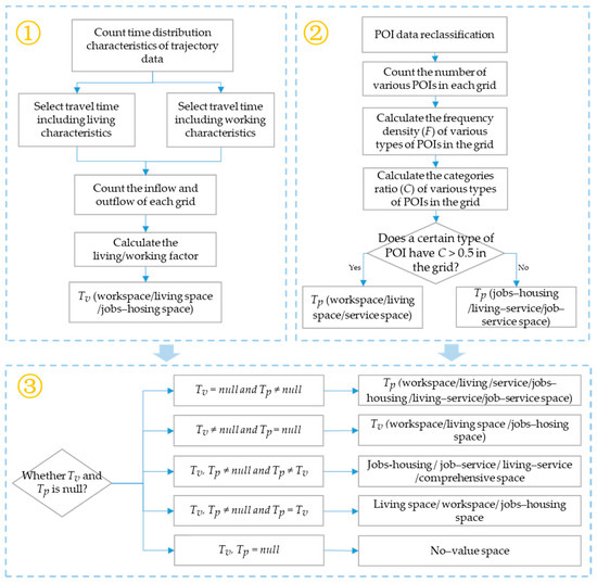
Figure 1.
Flowchart of the proposed method. F represents the frequency density. C represents the category ratio. Tv represents the recognition results from step1. Tp represents the recognition results from step 2.
3.1. Constructing the Travel Flow Model
3.1.1. Data Selection
The trajectory data contain travel records for 24 hours a day. This study analyzed the relationship between residents’ travel times and volumes on weekdays and weekends through the travel time–volume curve, and selected the dates and time that include the travel purpose of residence and work to filter and select travel data and construct an identification model for jobs-housing space.
As shown in Figure 2, the travel peak time occurs earlier on weekdays, and the travel time–volume curve is consistent with the daily travel characteristics of residents who work at sunrise and rest at sunset, so the morning and evening peaks are obvious. The travel peak times occur later on weekends, and the amount of travel is generally greater than the amount of travel during working days. Compared with weekday trips, weekend travel peaks appear in the afternoon. There are diverse travel purposes, making it difficult to capture the various working and living purposes. Therefore, we selected the weekday trip data to construct the model to identify jobs-housing space. According to the time characteristics of the travel peaks in the mornings and evenings of weekdays, we selected 5:00 ≤ t ≤ 9:00 a.m. and 17:00 ≤ t ≤ 19:00 as the morning and evening peak periods to determine the subsequent living and working factors.
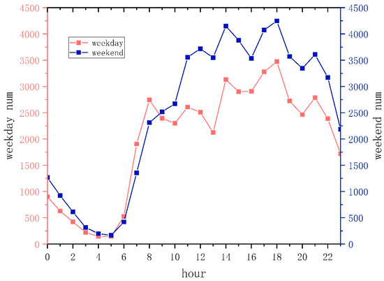
Figure 2.
Resident commuting time–volume chart for weekdays/weekends.
3.1.2. Recognition Model of Living Space
Due to the diversity of passenger destinations during evening rush hours, this study identified living space based on the travel trajectory during the morning rush hour. Based on Figure 2, 5:00 ≤ t ≤ 9:00 a.m. was selected as the morning peak period. When the residents’ travel time lies within this period, the generated trajectory can be used to identify the living space. Next, we count the inflow and outflow of passengers in each grid unit during this period and construct the living factor (LF) to identify the living space. Specifically, LF can be expressed as the difference between the inflow and outflow of passengers in each grid unit during the morning rush hour. LF is expressed as
where LFi is the living factor of the grid i. Since the results of the living spaces identified based on the working days were quite different, this study used a rule-based method to synthesize the identification results of the 21 working days in September 2017. Specifically, we calculated the average number of passenger inflows and outflows during the morning rush periods of 21 working days in each grid and ultimately calculated the living factor of each grid to identify the living space. Here, numin,i and numout,i respectively represent the average number of passenger inflows and outflows in grid i during the morning rush hours of the 21 working days. According to the travel characteristics of morning rush hours on weekdays, when LFi < 0, the outflow of passengers during the morning rush hour in the grid is greater than the inflow, reflecting the residential characteristics. When LFi > 0, the inflow of passengers during the morning rush hour in the grid is greater than the outflow, reflecting other characteristics, such as service characteristics, because the inflow of population in supermarkets, schools, and other service facilities is greater than the outflow during morning rush hours.
LFi = numin,i − numout,i
numin,i = (numin,i,1 + numin,i,2 + …… + numin,i,m)/m
numout,i = (numout,i,1 + numout,i,2 + …… + numout,i,m)/m
3.1.3. Recognition Model of Workspace
Based on Figure 2, 17:00 ≤ t ≤ 19:00 was selected as the evening rush hours. When the residents’ travel time is within the evening rush hours, the generated trajectory can be used to identify the workspace. Next, we count the inflow and outflow of passengers in each grid unit during the evening rush hours and calculate the working factor (WF) in each grid—that is, the difference between the inflow and outflow of passengers during the evening rush hours, which is used to identify the workspace. WF is expressed as:
where WFi is the working factor of the grid i; since the results of the workspace identified based on the workdays are quite different, this study uses a rule-based method to synthesize the identification results of the 21 workdays in September 2017. Specifically, we calculated the average number of passenger inflows and outflows during the evening rush hours of the 21 working days in each grid and then calculated the working factor of each grid to identify the workspace. Here, numin,I and numout,i respectively represent the average number of passenger inflows and outflows in grid i during the peak hours of the 21 working days. According to the travel characteristics of the evening rush hours of the working days, when WFi < 0, the outflow of passengers during the evening rush hours of the grid is greater than the inflow, reflecting the working characteristics; when WFi > 0, the inflow of passengers during the evening rush hours of the grid is greater than the outflow, reflecting other characteristics, such as service characteristics, because the inflow of population in restaurants, entertainment venues, and other service facilities is greater than the outflow during evening rush hours.
WFi = numin,i − numout,i
numin,i = (numin,i,1 + numin,i,2 + …… + numin,i,m)/m
numout,i = (numout,i,1 + numout,i,2 + …… + numout,i,m)/m
3.2. POI Quantitative Identification Method Construction
Previous studies indicated that POI data can be effectively applied to illustrate functional regions [31]. To calculate the point density of each type of POI in all grids, we first allocated the POIs of each category in the grid. Then, for each grid cell, the functional properties were identified by constructing the frequency density (Fi) and the category ratio (Ci). The calculation formula is
where i represents the type of POI; ni represents the number of the ith type of POI in the unit; Ni represents the total number of the ith type of POI; Fi represents the frequency density of the ith type of POI in the total number of POIs; and Ci represents the category ratio of the frequency density of the ith type of POI to the frequency density of all types of POIs in the unit.
According to the formula, the frequency density and category ratio of the POIs in each grid cell can be calculated. We selected the category ratio value of 0.5 as the criterion for judging the functional properties of the cell. When the category ratio of a certain type of POI in the grid cell is 0.5 or above, the grid unit is considered a single functional area for this type of POI, and when the category ratios of all types of POIs in the grid unit do not reach 0.5, the functional area is determined to be a mixed functional area. The mixed type instead depends on the two main POI types in the grid unit. When the grid cell does not contain a POI, the category ratio is null. This type of grid cell is called a valueless area.
Figure 3 illustrates the quantitative identification method for POIs. Table 1 shows the frequency density and the category ratios of various POIs in the two grids. The category ratio of C1 in grid 1 is more than 0.5, so grid 1 is determined to be a functional area of C1. There are no POIs in grid 2 with a category ratio greater than 0.5. Therefore, grid 2 is a mixed functional area, and the ratio of C3 and C4 is the highest. Therefore, grid 2 is considered as a mixed functional area of C3 and C4.
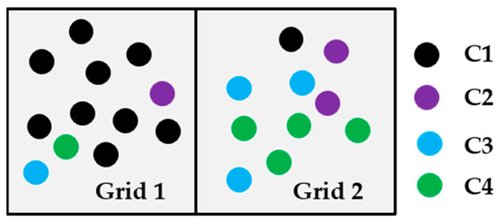
Figure 3.
Illustration of point-of-interest (POI) semantics for functional regions.

Table 1.
POI frequency density (FD) and category ratio (CR) of Figure 3.
3.3. Construction of a Travel Flow Model Considering the Spatial Distribution of Public Facilities
The travel flow model is based on the location data of the pick-up and drop-off points and is used to calculate the flow differences to identify the jobs-housing space. This method only considers the inflows and outflows of passengers in a certain period of the grid. This identification process does not consider the distribution of public facilities in the area, so the recognition results may be over-recognized. For example, consider a large scenic area in a grid. Tourists, as important passengers of Didi Chuxing, will migrate to other areas during the evening rush hours. If only the inflow of the area is considered, this area would likely be recognized as a workspace. Bars, nightclubs, KTVs, and other typical entertainment venues are usually open from 11:00 p.m. to 5:00 or 6:00 a.m. The morning rush hour is thus the off-duty time of the staff in such places. Consequently, the outflow in this area is generally greater than the inflow. If only the trajectory data are considered, this area is likely to be recognized as a living space. Therefore, POI data that can reflect the spatial distribution of public facilities were added to construct a flow model that considers the spatial distribution of public facilities to reduce over-recognition and improve recognition accuracy.
The basic concept of a travel flow model considering the spatial distribution of public facilities is as follows. Firstly, the model determines whether the result of a grid identified by the two methods is a non-value area. If the recognition result of the travel flow model is a non-value area and the POI quantitative identification result is not empty, the final result is the POI quantitative identification result; if the POI quantitative recognition result is a non-value area, and the recognition result of the travel flow model is not empty, then the final result is the recognition result of the travel flow model; if the recognition results of a grid identified by both methods are non-value areas, the grid belongs to the non-value area. Secondly, if the recognition results of the two methods are not empty, we compare whether the recognition results of the travel flow model and the POI quantitative identification method in each grid unit are consistent. If the results are consistent, the area is considered to be a functional area of the current types, and the recognition results include all three types of spaces: workspaces, living spaces, and jobs-housing spaces; if the results are inconsistent, the grid is considered to be a mixed functional area, and the recognition results include 4 types of space: jobs-housing space, job–service space, living–service space, and comprehensive space which is a multifunctional space, in which two or more urban functions are mixed to realize the diversity of urban functions, as shown in the following formula:
where Tf represents the final recognition result; Tv represents the recognition results of the travel flow based on trajectory data; Tp represents the recognition results of the POI quantitative recognition method; S represents the final recognition results when the result of the travel flow model is consistent with the results of the POI quantitative recognition method, mainly including living space, workspace, and jobs-housing space; M represents the final recognition result when the result of the travel flow model is not consistent with the results of the POI quantitative recognition method, mainly including four types: jobs-housing space, job–service space, living–service space, and comprehensive space.
3.4. Accuracy Evaluation
Since jobs-housing spaces are two important components of urban functional areas, the identification of jobs-housing space is a special case of urban functional area identification. The urban functional area is the distribution space of various functional activities within the city. At present, there is no official standard classification data of the urban functional areas. Therefore, the verification of identification accuracy of urban functional areas in existing studies usually adopts the methods of manual identification, comparison to the online map, and qualitative description [14,25,26]. To verify the usability of the jobs-housing space recognition method proposed here, the accuracy of the recognition results is evaluated by the method of coincidence scoring evaluation [32] with reference to online maps of the network, including Gaode map and Baidu Street View Map. This method then manually recognizes the real function type of the sample grid and compares it with the results identified by the method proposed in this article. According to the pre-set scoring rule, this method scores the conformity of the recognition results. Finally, the recognition results are scored according to the pre-set scoring rules, and the recognition accuracy is calculated. The specific scoring rules for each type of functional area are shown in Table 2. When the score of a certain functional area is 3, the type of functional area identified by the method here is the same as the real land-use type; 2 means nearly correct; 1 means slightly correct, and 0 means completely incorrect. The recognition accuracy is calculated as follows:
where P is the recognition accuracy rate; n is the total number of samples selected; xi is the conformity score of the functional area, and Xi is the full score of the functional area.
Table 2.
Scoring rules.
4. Case Study
4.1. Study Area and Data
4.1.1. Study Area
Haikou City, the capital city of Hainan Province, has a total area of 3145.93 km2, including a land area of 2284.49 km2 and a sea area of 861.44 km2. It is the political, economic, technological, and cultural center of Hainan Province and the largest transportation hub. It is also a fulcrum city of the national "One Belt One Road" strategy. This article takes the main urban area of Haikou City as its study area, which has jurisdiction over 21 streets, including Jinmao Street (JM), Zhongshan Street (ZS), and JinYu (JY).
To reflect the distribution of urban jobs-housing space reasonably, the study area should be divided into appropriate research units. The common research units include regular grid and traffic analysis zones (TAZ) divided by road networks. This paper is based on using trajectory data to study an urban jobs-housing space identification method. The trajectory data after coordinating corrections were mainly distributed on the urban road network. If the traffic analysis zone was used as the research unit, it would be impossible to infer which traffic analysis zones the trajectory data distributed on the road belong to. Therefore, we considered 500 m as the research diameter and divided the whole study area into regular grids (500 × 500 m2). The grid size was determined after preliminary experiments based on different grid resolutions. Ultimately, 828 grids were obtained, as shown in Figure 4.
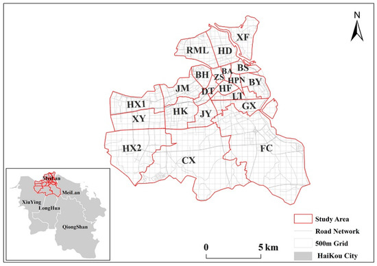
Figure 4.
Study Area. BS, BaiSha Street; BL, BaiLong Street; BH, BinHai Street; BA, BoAi Street; CX, ChengXi Town; DT, DaTong Street; FC, FuCheng Town; GX, GuoXing Street; HD, HaiDian Street Street; HF, HaiFu Street; HK, HaiKen Street; Hx1, HaiXiu Street; Hx2, HaiXiu Town; HPN, HePingnan Street; JinMao Street; JinYu Street; LanTian Street; RML, RenMinglu Street; XX, XiXiu Town; XF, XinFu Town; XY, XiuYing Street.
4.1.2. Study Data and Preprocessing
- Data Source
The trajectory data were obtained from the GAIA open dataset (https://gaia.didichuxing.com, accessed on 23 December 2020) of DiDi ChuXing, which is a data opening plan that was launched by Didi Chuxing in October 2017. DiDi ChuXing is a travel platform for the taxi, private car, express, driving, and bus services. DiDi ChuXing has altered the traditional method of taking a taxi and led the development of modern travel in the era of mobile internet [14]. We selected the 30-day trajectory data of Haikou from September 1st to September 30th, 2017 as the research data. These data mainly contain attribute data such as the order ID, product line ID, city ID, city area code, secondary counties, departure time, arrival time, latitude and longitude of the departure location, and latitude and longitude of the arrival location.
POI data were acquired from the open platform of Gaode Map (https://lbs.amap.com, accessed on 23 December 2020), a leading provider of digital map, navigation, and location services in China. By dividing the main urban area of Haikou into regular grids (2000 × 2000 square meters), we captured the POI data using Visual Studio 2015 software platform based on the C# language. Finally, 15,643 records of POIs data in Haikou were obtained. These data included serial number, name, address, category, district and county, capture time, and latitude and longitude information.
- Data Processing
The trajectory data were recorded by a device with GPS positioning functions and wireless communication equipment installed in the traveling vehicle. Errors in the recording of the instrument or errors in the driver’s operations may cause data errors. To make the research results more accurate, we used Python tools to process the noise data in the raw data. The speed threshold method was mainly used to filter the original data. The speed value was determined by the ratio of the travel distance to the travel time. The driving speed in the urban area is usually greater than 10 km/h, and the maximum speed limit of the expressway is selected as 120 km/h. Therefore, 10 and 120 were set as the upper and lower thresholds for data cleaning. Then, the travel records with an average speed of less than 10 km/h and greater than 120 km/h were eliminated to obtain travel trajectory data that conformed to the actual situation.
The GaoDe POI classification includes eighteen categories. The purpose of this study was to identify jobs-housing space, so we excluded two types of POIs (“Road ancillary facilities” and “Place name address information”) that were irrelevant to the jobs-housing space and reclassified other POIs categories into three new categories: employment, residence, and services. A comparison of the POI data categories before and after reclassification is presented in Table 3.
Table 3.
Categories of POIs.
4.2. Recognition Result of the Travel Flow Model
Based on the travel flow model, three types of results were obtained, namely workspace, living space, and jobs-housing space. As shown in Figure 5, there are 304 grids of workspace, accounting for 15.7% of the total number of grids in the study area; 210 grids of living space, accounting for 10.8% of the total number of grids in the study area; and 303 grids of jobs-housing space, accounting for 15.6% of the total number of grids in the study area. The remaining grids are areas with no value. In general, the workspace grids comprise the largest proportion, and the residential grids comprise the smallest proportion.
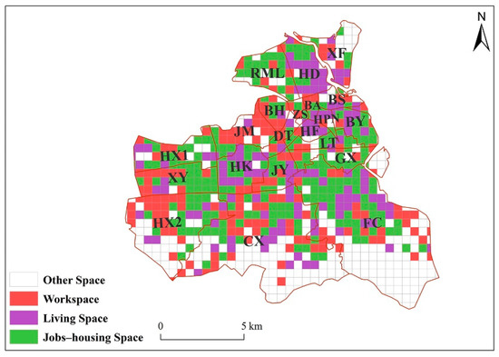
Figure 5.
Recognition results of the travel flow model.
As shown in Table 4, the statistics of the spatial distribution of various types of functional areas show that high-density workspaces are mainly distributed on the BH, DT, JM, JY, and ZS streets, among which BH has the highest density with a value of 4.31; high-density living spaces are concentrated on the BH, HD, HF, HK, and JY streets, among which JY has the highest density with a value of 3.80. The high-density jobs-housing spaces are mainly distributed on the BL, GX, HPN, JY, and LT streets, among which LT has the highest density with a value of 6.24.
Table 4.
Statistics on the number and density (/km2) of street land types.
Comparing the proportions of various types of grids in each street, the results show that 9 streets, BH, DT, HX2, JM, LS, XX, YF, CL, and ZS, are workspace; the 6 streets of BS, BA, HD, HF, HK, and XF are living space; and the 10 streets of BL, CX, FC, GX, HX1, HPN, JY, LT, RML, and XY are jobs–housing.
4.3. POI Quantitative Identification Method Identification Results
The quantitative POI identification results according to the formula (3.7–3.8) are shown in Figure 6. There are 236 grids of workspace, accounting for 12.18% of the total number of grids in the study areas; 289 grids of living space, accounting for 14.92% of the total number of grids in the study areas; 236 grids of service space, accounting for 12.18% of the number of grids in the study areas; 50 grids of living–service space, accounting for 0.26% of the total number of grids in the study area; 55 grids jobs-housing space, accounting for 0.28% of the total number of grids in the study area; and 49 grids of work–service space, accounts for 0.03% of the total number of grids in the study area. By comparing the proportions of various functional areas, it is found that the grids of living space account for the largest proportion, while the grids of living–service space account for the smallest proportion.
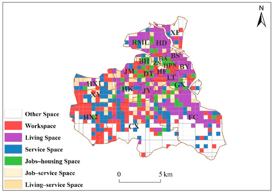
Figure 6.
Recognition results of the POI quantitative recognition.
As outlined in Table 5, the statistics of the spatial distribution of various functional areas indicate that workspaces with high density are mainly distributed on the DT, HF, HPN, LT, and ZS streets, among which LT has the highest density with a value of 3.94; living spaces with high density are mainly distributed on the BL, BS, GX, HD, JY, and LT streets, among which JY streets have the highest density with a value of 6.34; service spaces with high density are mainly distributed on streets such as HX1, HX2, XY, etc., among which XY streets have the highest density with a value of 2.05; jobs-housing spaces with high density are mainly distributed on streets such as BH, DT, and HPN, among which HPN streets have the highest density with a value of 5.34; job-service spaces with high density are mainly distributed on the streets of BA, XY, and ZS, among which BA streets have the highest density with a value of 3.64; living–service spaces with high density are mainly distributed on the HX1, HK, and JY streets, among which the JY street has the highest density with a value of 1.77. On the whole, the density value of the living area on each street is relatively high, the density value of the living–service space on each street is relatively low, and the highest density value of the residential area is 3.6 times that of the highest density value of the living–service mixed area.
Table 5.
Statistics on the number and density (/km2) of street land types.
Comparing the proportions of various types of grids in each street, the results show that the streets of CX, HX2, and LS are workspaces. The streets of BL, BS, FC, GX, HD, HF, HK, JM, JY, LT, RML, XF, and YF are living spaces. The streets of HX1, XX, and CL service spaces. The streets of BH, DT, and HPN are jobs-housing spaces. The streets of BA and ZS are work–service spaces. These streets do not feature living–service spaces. Overall, the quantitative recognition results of the POI show that more than 50% of the streets are mainly of residential types.
4.4. Recognition Results of the Travel Flow Model Considering the Spatial Distribution of Public Facilities
The identification results of the travel flow model considering the spatial distribution of public facilities are shown in Figure 7. In this figure, 282 grids are workspaces, accounting for 14.56% of the total number of grids in the study area; 200 grids are living spaces, accounting for 10.33% of the total number of grids in the study area; 104 grids are service spaces, accounting for 5.37% of the total number of grids in the study area; 294 grids are jobs-housing spaces, accounting for 15.18% of the total number of grids in the study area; 74 grids are job–service spaces, accounting for 3.82% of the total number of grids in the study area; 43 grids are living–service spaces, accounting for 2.22% of the total number of grids in the study area; and 114 grids are comprehensive spaces, accounting for 5.89% of the total number of grids in the study area. Among the seven results, the workspace has the largest proportion, while living–service space has the smallest proportion. Compared to the new results from the travel flow model, the number of work, living, and jobs-housing spaces is reduced, and four new functional space types have appeared—namely, service space, job–service space, living–service space, and comprehensive space. Compared to the new results from the POI quantitative identification method, the number of working, jobs-housing, and job–service spaces increased, but the number of living, service, and living–service space reduced, and a new type of functional area is added: comprehensive space. As shown in Table 6, the functional region of Haikou City is dominated by a single functional region, but the difference in the number of the two types of functional areas is small. Specifically, the single functional region accounts for 52.75%, and the mixed functional region accounts for 47.25%. The main single functional region is the workspace, and the main mixed functional region is the jobs-housing space.
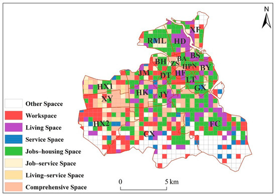
Figure 7.
Recognition results of the travel flow model considering the spatial distribution of public facilities.
Table 6.
Comparison of the recognition results of the three methods.
As shown in Table 7, the statistics on the spatial distribution of various functional areas show that workspaces with high density are mainly distributed on the DT, HF, JM, XY, and ZS streets, among which the DT has the highest density with a value of 2.60. Living spaces with high density are mainly distributed on the BS, HD, HK, JY, and LT streets, among which the JY street has the highest density with a value of 3.80. Service spaces with high density are mainly distributed on the DT street, with a value of 1.30. Jobs-housing spaces with high density are mainly distributed on the DT, GX, HPN, JY, and LT streets, among which the HPN street has the highest density with a value of 8.90. Job–service spaces with high density are mainly distributed on the BH, JY, and ZS streets, among which the BH street has the highest density with a value of 1.80. Living–service space with high density is mainly distributed on the BA and HX1 streets, among which the BA street has the highest density with a value of 0.91. Comprehensive space with high density is mainly distributed on the BA, HK, HX1, XY, and ZS streets, among which the XY street has the highest density with a value of 3.45. Overall, the density value of the jobs-housing space in each street is relatively high, the density value of living–service space in each street is relatively low, and the highest density value of jobs-housing space is nine times that of the highest density value of living–service space.
Table 7.
Statistics on the number and density (/km2) of street land types.
Comparing the proportions of various types of grids in each street, the results show that there are three types of functional districts at the street level in Haikou City—namely, jobs-housing space, workspace, and comprehensive space. Most streets belong to the jobs-housing space, including BL, BS, BH, CX, DT, and 11 other streets; HX2, LS, XX, YF, and CL are workspace; and BA, HX1, XY, and ZS are comprehensive space. No streets belong to the other four types of functional space.
4.5. Accuracy Evaluation
In total, 286 grid samples in the study area were randomly selected to verify the recognition accuracy. Since 16 grids of the 286 selected samples feature no POI distribution and belong to the valueless area, 270 sample grids were available for the quantitative POI identification method. A total of 43 grids lacked dripping travel data distribution and were also non-valued areas. Therefore, 243 sample grids were available for the mobile travel volume model. Table 8 shows the scores of all samples and the overall recognition accuracy of each method. The recognition accuracy of the method proposed here is 85.90%, and the recognition accuracy of the travel flow model and the POI quantitative recognition method is 72.43% and 74.94%, respectively. The accuracy of the method proposed here is significantly higher than that of the other two methods, while the accuracy of the travel flow model is the lowest. Based on the results of the accuracy evaluation, the method proposed here can obtain high recognition accuracy and accurately identify the spatial distribution of urban jobs–housing, which will be helpful for subsequent research on jobs-housing balance.
Table 8.
Comparison of the recognition accuracy rates of different methods.
5. Conclusion and Discussion
Urban jobs-housing space is an important part of a city’s spatial structure and morphological characteristics, affecting the normal operations of urban functions and the commuting modes of residents. Identifying and analyzing the spatial distribution of urban jobs-housing space formed at this stage can help to evaluate the urban jobs-housing relationship, find out the unreasonable places in the existing urban space, and provide a reference for the subsequent rational planning of urban space. Therefore, this paper proposed a travel flow model by integrating trajectory data and urban POI data, which considers the spatial distribution of POIs to identify urban jobs-housing spaces. This model comprehensively considers the dynamic commuting characteristics of urban people and the static spatial distribution characteristics of various urban facilities. We also solved the problem of over-identification caused by using a single travel data sources and the problem of inaccurate identification due to the shortcomings of POI data, such as slow updates and a weak current status. To assess the feasibility and accuracy of the model, we selected 21 streets in Haikou as the study area for verification. (1) The results of the accuracy evaluation showed that the identification accuracy of the travel flow model and the POI quantitative identification method is 72.43% and 74.94%, respectively. The accuracy of the method proposed in this article is 85.90%, which is higher than that of the method using a single data source. (2) The functional region of Haikou City is dominated by workspaces and jobs-housing spaces, but the density of the latter is greater than that of the former. Therefore, the method proposed here can serve as a reference for future research on urban jobs-housing space.
We combined trajectory data and urban POI data to identify jobs-housing spaces. Although the accuracy of the recognition of the method improved compared to research using a single data source, there are still some limitations in this study: (1) the precision of jobs-housing space identification highly depends on the quantity of data. The trajectory data used in this study was collected from Didi Chuxing, however, not all people commute using Didi Chuxing, which brings about a problem of deviation in user samples and affects the recognition results. (2) The quantitative POI identification method in the identification model constructed in this study only considered the frequency density and the category ratios of POIs, ignored other attributes such as facility area, which affects the accuracy of identification. For example, suppose that many residential communities are distributed in a grid, and supporting infrastructure such as supermarkets, barbershops, pharmacies, etc. are distributed around the residential areas. If the functional area is identified by the POI quantitative identification method, the number of POIs of each type needs to be calculated. Since the residential area distributed in the grid may belong to the same community, the number of residential POIs is significantly less than the number of service POIs, the grid is likely to be identified as the service space. (3) To verify the accuracy of the recognition results of the jobs-housing space, this study referred to the Gaode map and the street view map to obtain the true functional attributes of 286 sample grids through manual visual interpretation, although the results obtained by it can more accurately reflect the real world, this method requires a lot of time and labor cost, and is not suitable when the research scope is large. (4) Since grids are used as the basic research unit in this study, the result of job-housing space recognition is easily affected by the Modifiable Areal Unit Problem (MAUP). To reduce the influence of MAUP on the recognition result, an ideal spatial analysis unit must be selected depending on the specific conditions of the study area.
Therefore, future research can improve in the following ways: (1) Add multi-source data. In subsequent research, adding mobile phone data, bus/subway card data, and other types of GPS travel trajectory data with large samples would solve the problem of the single user group and small sample size and improve recognition accuracy. (2) Introduce building area attributes of POI data, the areas of various types of POIs are an important factor in identifying the functional type of the area, subsequent research could use area of interest (AOI) data to calculate the building area and use that area as a weight to identify jobs-housing spaces more accurately. (3) Subsequent research needs to develop a verification method for the identification results of the jobs-housing space, which not only needs to be easy to implement but also truly reflects the accuracy of the identification results. (4) Subsequent research can analyze the degree of influence of MAUP on the recognition model proposed in this paper by calculating the accuracy of the recognition results of jobs-housing space under different spatial scales and find an ideal spatial analysis unit to reduce the influence of MAUP.
Author Contributions
Data curation, Yong Wang; methodology, Ya Zhang; project administration, Jiping Liu; resources, Jiping Liu; writing—original draft, Ya Zhang; writing—review and editing, Yungang Cao and Youda Bai. All authors have read and agreed to the published version of the manuscript.
Funding
This work was supported in part by the National Key Research and Development Plan of China (under project numbers 2017YFB0503601 and 2017YFB0503502), the Basic Business Cost Project for Central-level Scientific Research Institutes (AR2011) and Basic surveying and mapping project (AR2004).
Conflicts of Interest
The authors declare no conflict of interest.
References
- Levine, J.C. Rethinking Accessibility and Jobs-Housing Balance. J. Am. Plan. Assoc. 1998, 64, 133–149. [Google Scholar] [CrossRef]
- Wu, W. Migrant Intra-urban Residential Mobility in Urban China. Hous. Stud. 2006, 21, 745–765. [Google Scholar] [CrossRef]
- Jinping, S.; Enru, W.; Wenxin, Z.; Peng, P. Housing suburbanization and employment spatial mismatch in Beijing. Acta Geogr. Sin. 2007, 62, 387–396. [Google Scholar]
- Zhou, J.; Wang, Y.; Cao, G.; Wang, S. Jobs-housing balance and development zones in China: A case study of Suzhou Industry Park. Urban Geogr. 2016, 38, 363–380. [Google Scholar] [CrossRef]
- Liu, W.; Hou, C. Urban Residents’ Home-work Space and Commuting Behavior in Guangzhou. Sci. Geogr. Sin. 2014, 34, 272–279. [Google Scholar]
- Deng, Y.; SI, Y. The spatial pattern and influence factors of urban expansion: A case study of Beijing. Geogr. Res. 2015, 34, 2247–2256. [Google Scholar]
- Song, X.; Wang, Y.; Yang, Y.; Zhang, K.; Niu, X. Statistical Verification of Home-Work Separation based on Commuting Distance. J. Geo-Inf. Sci. 2019, 21, 1699–1709. [Google Scholar]
- Liu, Y.; Chen, L.; An, Z.; Zhang, X. Research on Job-Housing and Commuting in Wuhan based on Bus Smart Card Data. Econ. Geogr. 2019, 39, 93–102. [Google Scholar]
- Liu, D.; Yang, Y.; Zhu, C. Characteristics of jobs-housing spatial organization in Lanzhou City. Arid Land Geogr. 2012, 35, 288–294. [Google Scholar]
- Sultana, S. Job/Housing Imbalance and Commuting Time in the Atlanta Metropolitan Area: Exploration of Causes of Longer Commuting Time. Urban Geogr. 2002, 23, 728–749. [Google Scholar] [CrossRef]
- Li, M.; Kwan, M.; Wang, F.; Wang, J. Using points-of-interest data to estimate commuting patterns in central Shanghai, China. J. Transp. Geogr. 2018, 72, 201–210. [Google Scholar] [CrossRef]
- Wang, D.; Li, D.; Fu, Y. Employment space of residential quarters in Shanghai: An exploration based on mobile signaling data. Acta Geograhica Sin. 2020, 75, 1585–1602. [Google Scholar]
- Zou, Q.; Yao, X.; Zhao, P.; Wei, H.; Ren, H. Detecting home location and trip purposes for cardholders by mining smart card transaction data in Beijing subway. Transportation 2018, 45, 1–26. [Google Scholar] [CrossRef]
- Liu, X.; Tian, Y.; Xue, Z.; Wan, Z. Identification of Urban Functional Regions in Chengdu Based on Taxi Trajectory Time Series Data. ISPRS Int. J. Geo-Inf. 2020, 9, 158. [Google Scholar] [CrossRef]
- Wang, B.; Wang, L.; Liu, Y.; Yang, B.; Huang, X.; Yang, M. Characteristics of jobs-housing spatial distribution in Beijing based on mobile phone signaling data. Prog. Geogr. 2020, 39, 2028–2042. [Google Scholar] [CrossRef]
- Zhou, Z. Study on the job-housing spatial characteristics in Zhuhai based on mobile location data. World Reg. Stud. 2020, 29, 1172–1180. [Google Scholar]
- Alexander, L.; Jiang, S.; Murga, M.; Gonzalez, M.C. Origin–destination trips by purpose and time of day inferred from mobile phone data. Transp. Res. Part C Emerg. Technol. 2015, 58, 240–250. [Google Scholar] [CrossRef]
- Isaacman, S.; Becker, R.; Cáceres, R.; Kobourov, S.; Martonosi, M.; Rowland, J.; Varshavsky, A. Identifying Important Places in People’s Lives from Cellular Network Data. In Proceedings of the Pervasive Computing, Heidelberg, Germany, 12–16 September 2011; pp. 133–151. [Google Scholar]
- Liu, X.; Dong, L.; Jia, M.; Tan, J. Urban Jobs-Housing Zone Division Based on Mobile Phone Data. In Blockchain and Trustworthy Systems; Springer: Guangzhou, China, 2020; pp. 534–548. [Google Scholar]
- Ahas, R.; Aasa, A.; Silm, S.; Tiru, M. Daily rhythms of suburban commuters’ movements in the Tallinn metropolitan area: Case study with mobile positioning data. Transp. Res. Part C Emerg. Technol. 2010, 18, 45–54. [Google Scholar] [CrossRef]
- Long, Y.; Thill, J.-C. Combining smart card data and household travel survey to analyze jobs-housing relationships in Beijing. Comput. Environ. Urban Syst. 2013, 53, 19–35. [Google Scholar] [CrossRef]
- Sari Aslam, N.; Cheng, T.; Cheshire, J. A high-precision heuristic model to detect home and work locations from smart card data. Geo-Spat. Inf. Sci. 2018, 22, 1–11. [Google Scholar] [CrossRef]
- Han, Z.; Cui, C.; Miao, C.; Wang, H.; Chen, X. Identifying Spatial Patterns of Retail Stores in Road Network Structure. Sustainability 2019, 11, 4539. [Google Scholar] [CrossRef]
- Jiang, S.; Alves, A.; Rodrigues, F.; Ferreira, J.; Pereira, F.C. Mining point-of-interest data from social networks for urban land use classification and disaggregation. Comput. Environ. Urban Syst. 2015, 53, 36–46. [Google Scholar] [CrossRef]
- Yi, D.; Yang, J.; Liu, J.; Liu, Y.; Zhang, J. Quantitative Identification of Urban Functions with Fishers’ Exact Test and POI Data Applied in Classifying Urban Districts: A Case Study within the Sixth Ring Road in Beijing. ISPRS Int. J. Geo-Inf. 2019, 8, 555. [Google Scholar] [CrossRef]
- Yu, B.; Wang, Z.; Mu, H.; Sun, L.; Hu, F. Identification of Urban Functional Regions Based on Floating Car Track Data and POI Data. Sustainability 2019, 11, 6541. [Google Scholar] [CrossRef]
- Wu, Q.; Zhang, L.; Wu, Z. Identifying City Functional Areas Using Taxi Trajectory Data. J. Geomat. Sci. Technol. 2018, 35, 413–417 + 424. [Google Scholar]
- Zhao, P.; Cao, Y. Jobs-Housing Balance Comparative Analyses with the LBS Data: A Case Study of Beijing. Acta Sci. Nat. Univ. Pekin. 2018, 54, 1290–1302. [Google Scholar]
- Yao, Y.; Qian, C.; Hong, Y.; Guan, Q.; Chen, J.; Dai, L.; Jiang, Z.; Liang, X. Delineating Mixed Urban “Jobs-Housing” Patterns at a Fine Scale by Using High Spatial Resolution Remote-Sensing Imagery. Complexity 2020, 2020, 1–13. [Google Scholar] [CrossRef]
- Wang, L.; Chang, F. The study of job-housing relationship of city based on multisource big data-taking central urban area of lanzhou as an examplemain city area. Human Geogr. 2020, 35, 65–75. [Google Scholar]
- McKenzie, G.; Janowicz, K. The Effect of Regional Variation and Resolution on Geosocial Thematic Signatures for Points of Interest. In Societal Geo-Innovation; Springer: Cham, Switzerland, 2017; pp. 237–256. [Google Scholar]
- Kang, Y.; Wang, Y.; Xia, Z.; Chi, J.; Jiao, L.; Wei, Z. Identification and classification of wuhan urban districts based on POI. Geomat 2018, 43, 81–85. [Google Scholar]
Publisher’s Note: MDPI stays neutral with regard to jurisdictional claims in published maps and institutional affiliations. |
© 2021 by the authors. Licensee MDPI, Basel, Switzerland. This article is an open access article distributed under the terms and conditions of the Creative Commons Attribution (CC BY) license (http://creativecommons.org/licenses/by/4.0/).