Deep Learning for Toponym Resolution: Geocoding Based on Pairs of Toponyms

Abstract

Geocoding aims to assign unambiguous locations (i.e., geographic coordinates) to place names (i.e., toponyms) referenced within documents (e.g., within spreadsheet tables or textual paragraphs). This task comes with multiple challenges, such as dealing with referent ambiguity (multiple places with a same name) or reference database completeness. In this work, we propose a geocoding approach based on modeling pairs of toponyms, which returns latitude-longitude coordinates. One of the input toponyms will be geocoded, and the second one is used as context to reduce ambiguities. The proposed approach is based on a deep neural network that uses Long Short-Term Memory (LSTM) units to produce representations from sequences of character n-grams. To train our model, we use toponym co-occurrences collected from different contexts, namely textual (i.e., co-occurrences of toponyms in Wikipedia articles) and geographical (i.e., inclusion and proximity of places based on Geonames data). Experiments based on multiple geographical areas of interest—France, United States, Great-Britain, Nigeria, Argentina and Japan—were conducted. Results show that models trained with co-occurrence data obtained a higher geocoding accuracy, and that proximity relations in combination with co-occurrences can help to obtain a slightly higher accuracy in geographical areas with fewer places in the data sources.

1. Introduction

Geocoding is a core part of the broader text geoparsing task (also known as toponym resolution), in addition to geotagging. While geotagging deals with the automatic recognition of named entities (i.e., named entity recognition) corresponding to places, geocoding aims to match the identified place entities to the corresponding locations. Usually, the task consists of associating real-world coordinates (i.e., latitude-longitude) or polygon boundaries to toponyms. One important challenge in geocoding is related to toponym disambiguation [1] which faces, among other types of ambiguity issues [2], the problem of referent ambiguity (also known as geo/geo ambiguity). Referent ambiguity refers to toponyms having multiple locations [3] (e.g., Sofia (capital of Bulgaria) ≠ Sofia (province in Bulgaria)). Additionally, as gazetteer lookup methods are widely used for geocoding, gazetteer completeness (i.e., appropriate geospatial and temporal coverage) is also a major issue for the geocoding task. For instance, in the case of historical document analysis, new methods were proposed in order to geocode toponyms and solve toponym ambiguity without using gazetteers [4,5,6].

Place names are often grounded to their geographic area, and specific character sequences—e.g., prefixes and suffixes—can be found in close locations. For instance, place names in south-west of France tend to end with the suffix “-ac”. Character n-grams have been proven efficient for different natural language processing tasks, involving spelling errors or neologisms. Therefore , we propose a deep neural network architecture to model toponym co-occurrences in various contexts, combining n-gram embeddings with Long Short-Term Memory (LSTM) units (The code is available online: https://git.liris.cnrs.fr/jfize/toponym-geocoding (accessed on 28 November 2021)). The proposed architecture takes pairs of toponyms as input and returns latitude and longitude coordinates as outputs. For each pair, the first entry is the toponym that we want to geocode, and the second entry is used as context. This particular matching choice can easily adapt to different geocoding scenarios or applications (e.g., resolving place names referenced in textual paragraphs or place names appearing in tables or spreadsheets). We describe several experiments and evaluation results based on various contexts. For instance, we built several datasets of pairs of toponyms in order to evaluate the contribution of different relations between toponyms. We consider three types of relations, namely (1) co-occurrences of toponyms in text, based on Wikipedia articles describing geo-located places, (2) spatial proximity, computed from Geonames data and based on a buffer radius around each toponym, and (3) spatial inclusion, also computed from Geonames data and based on the feature type hierarchy (e.g., a city included in an administrative region).

This article is organised as follows: Section 2 presents related work, while Section 3 describes the proposed architecture and the data used for the model training. Section 4 presents several experiments and evaluation scores obtained on different datasets. Then, Section 5 discuss limitations in of our proposal, and Section 6 concludes the paper.

2. Related Work

We distinguish four categories of methods for geocoding: two using gazetteer matching with either heuristics or machine learning techniques, and two using no gazetteer data and leveraging language models or deep learning methods.

Several studies used map-based approaches or distance heuristics in combination with gazetteer lookup methods [1,7,8]. These methods are mainly based on the calculation of distance between place candidates and unambiguous toponyms. Lieberman et al., proposed to combine different spatial contexts: a global context that integrates knowledge from external datasets (i.e., gazetteers) and a local context that uses information extracted from the text itself [9]. In the context of hiking description analysis, Moncla et al. proposed a method based on the DBSCAN clustering algorithm (Density-Based Spatial Clustering) [10], grapping all toponym referents and then selecting the cluster of places that contains the maximum number of distinct toponyms [11]. Other heuristics, such as subtyping using feature type metadata, are also used. In addition to the spatial context (e.g., distance, proximity, density, centroid, etc.), methods involving other different types of heuristics (e.g., importance, size, population count, semantic or ontology hierarchical relations, etc.) have also been proposed [12,13,14].

Other data-driven approaches are also based on gazetteers and use machine learning instead of manually designed combinations of heuristics [15,16,17,18]. Hu and Ge used machine learning algorithms such as decision trees on a probability matrix between toponyms and place candidates. Each weight is computed by comparing geographical features of all candidates [15]. Lieberman and Samet proposed to use the combination of features from the toponym to be disambiguated and other toponyms that appears in a context window [16]. Molina-Villegas et al. proposed the use of word embedding for geographic named entity recognition and geographic entity disambiguation [17]. This approach aims to explore semantic relationships of words and documents in Mexican Spanish. They use Wikipedia articles of locations to enrich the semantic space of word embedding models with information from different topics such as culture, economy and history.

Several gazetteer-free methods have also been developed. Some of these are based on language models, defined in [19] as a model that “[...] assigns a probability of likelihood of a given word (or a sequence words) to follow a sequence of words”. In geocoding, approaches that use language models compute the probability of a word (or word sequence) to be associated with a geographic footprint. Delozier et al. propose to learn the probabilities for words (including toponyms) to be associated to a region, the latter being defined by rectangular area [4]. Kamallo and Rafieri use different language models learned on specific features, combining them to associate a ranking for each place candidate to a toponym [20]. Speriosu and Baldridge propose different geocoding algorithms, one based on geographical features only (from Geonames) and three text-driven approaches using a subset of Wikipedia, named GEOWIKI, that corresponds to articles for geographic places [21].

More recent studies rely on deep neural network architectures [22,23,24]. For instance, Gritta et al. proposed a network architecture that learns from multiple inputs: context words, context place mentions, and MapVec, i.e., a vector that encodes all place coordinates that share the same toponym as the input [22]. Cardoso et al. [23] combined context-aware word-embeddings [25] and a recurrent neural network based on Bidirectional LSTMs [26].

Context-based methods can obtain a high geocoding accuracy. However, most of these approaches require external resources (even after training) and are still based on analysis performed at the word level. They can thus be unfit for toponym variations or spelling errors. Considering these issues, our contribution lies on proposing a model that does not require a gazetteer and is trained on a subword level. In addition to reducing the impact of spelling errors, the use of sub-words (or character n-grams) has been known to be efficient in different natural language processing tasks. Most importantly, certain subwords can integrate spatial properties due to their usage. For instance, the prefix tre- is commonly used in Bretagne, FR because it means populated place in the local language. Additionally, in France, the suffix -ac is found almost exclusively in names of places located in the south west of France.

3. Materials and Methods

To address the problem of geocoding toponyms, we propose a neural network architecture that takes two toponyms as input and returns latitude and longitude coordinates corresponding the location of the first one. We chose to use only two toponyms because we want our model to geocode place names from data with few contextual information such as tabular data, historical documents, images or map captions) The two input toponyms are defined as follows: the first toponym t is the one to be geocoded. The second toponym $ct$ is a contextual toponym that helps to disambiguate t. The model can be defined as a function f such as $f(t,ct)\to (t_{lat},t_{lon})\in {\mathbb{R}}^2$ where $t_{lat}$ and $t_{lon}$ refer to the latitude and the longitude of t. For our model to adapt to toponym variations (aliases, spelling errors, etc.) and to learn geographic properties of certain affixes, input toponyms are transformed to sequences of character n-grams. For instance, if the sequence size n is 2, the toponym Paris will be represented as the following sequence: {Pa,ar,ri,is}. In this study, based on preliminary experiments, n is set to 4.

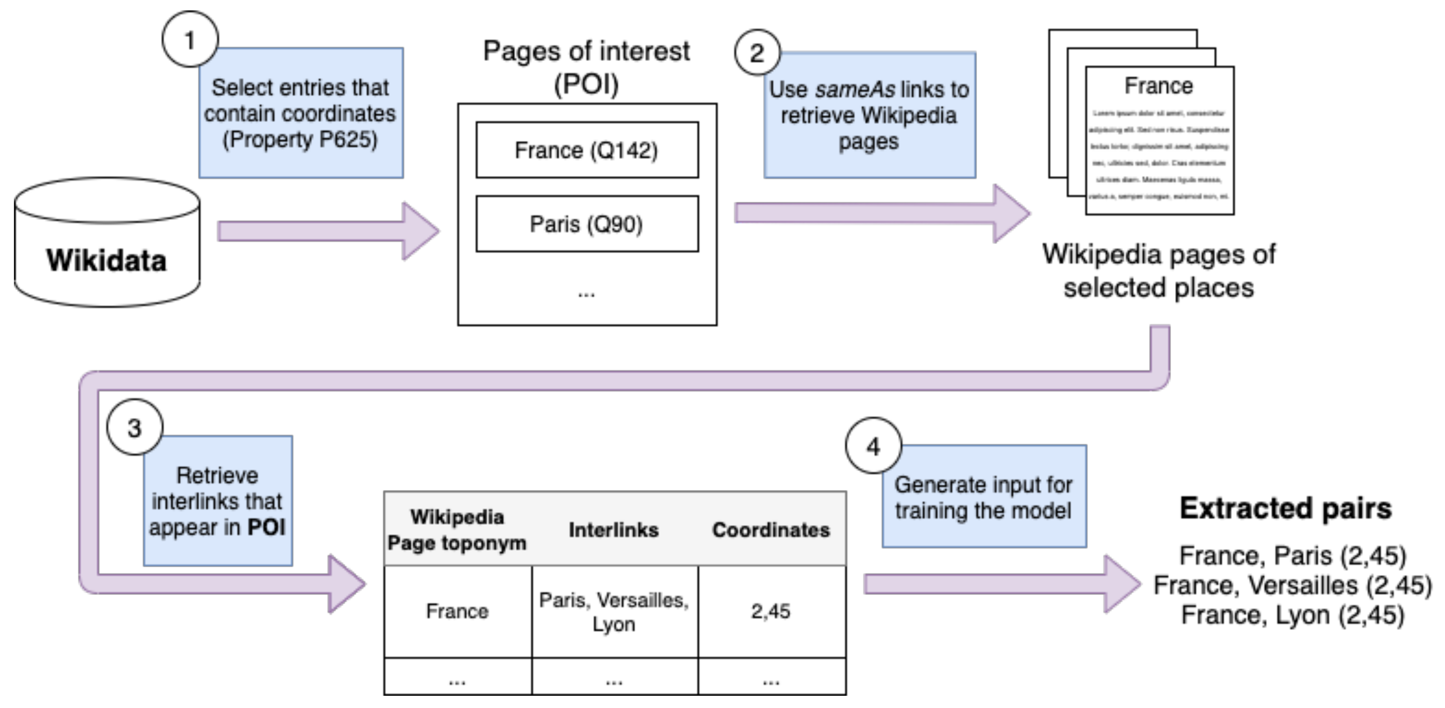
3.1. Process Overview

The process workflow is divided into three steps: (i) toponym transformation to character n-grams; (ii) latitude-longitude prediction using a recurrent neural network architecture; (iii) reprojecting output coordinates into the WGS84 (https://fr.wikipedia.org/wiki/WGS_84 (accessed on 28 November 2021)) coordinate system.

The first step takes and transforms each input toponym into a character n-gram sequence. In order to be compatible with the neural network, we need to assign each n-gram to a row in an embedding matrix, which contains vector representations for a defined vocabulary, e.g., a set of words or word n-grams. In our approach, this corresponds to every n-gram found in a large set of toponyms collected from both Geonames and Wikipedia in multiple languages. N-gram embeddings are generated using the Word2vec Skip-gram model [27]. As a first experiment, we did not use more recent approaches like ELMo or BERT because these embeddings are contextualized on larger textual utterances (e.g., sentences), whereas we do not use much textual context in our approach (only two toponyms, and not entire sentences as in several other NLP studies).

Once the input is transformed, the next step consists of predicting the coordinates using the neural network illustrated in Figure 1. This neural network is divided into two parts, with one responsible for the feature extraction (i.e., a Bidirectional LSTM), and the second responsible for predicting coordinates using the extracted features. Bi-LSTM or Bidirectional LSTM networks are well known for their efficiency in extracting features from sequential data. The LSTM cell formula is as follows:

$$\begin{array}{cc}\hfill f_t& ={\sigma }_g(W_f{x}_t+U_f{h}_{t-1}+b_f),\hfill \\ \hfill i_t& ={\sigma }_g(W_i{x}_t+U_i{h}_{t-1}+b_i),\hfill \\ \hfill o_t& ={\sigma }_g(W_o{x}_t+U_o{h}_{t-1}+b_o),\hfill \\ \hfill {\tilde{c}}_t& ={\sigma }_c(W_c{x}_t+U_c{h}_{t-1}+b_c),\hfill \\ \hfill c_t& =f_t\circ c_{t-1}+i_t\circ {\tilde{c}}_t,\hfill \\ \hfill h_t& =o_t\circ {\sigma }_h\left(c_t\right),\hfill \end{array}$$

where $x_t\in {\mathbb{R}}^d$ is the input vector to the LSTM unit; $f_t\in {\mathbb{R}}^h$ is a forget gate’s activation vector; $i_t\in {\mathbb{R}}^h$ is the input/update gate’s activation vector; $o_t\in {\mathbb{R}}^h$ is hte output gate’s activation vector; $h_t\in {\mathbb{R}}^h$ is the hidden state vector also known as output vector of the LSTM unit; ${\tilde{c}}_t\in {\mathbb{R}}^h$ is the cell input activation vector; $c_t\in {\mathbb{R}}^h$ is the cell state vector; $W\in {\mathbb{R}}^{h\times d}$, $U\in {\mathbb{R}}^{h\times h}$ and $b\in {\mathbb{R}}^h$ are weight matrices and bias vector parameters which need to be learned during training.

Bi-LSTMs are frequently used in NLP for named entity recognition [26,28] or for producing contextual word-embeddings [25]. Once the features are extracted by the Bi-LSTM, we use two multi-layer perceptrons, one for predicting each coordinate (latitude and longitude). Each one is composed of two layers of 500 neurons with a ReLU activation function [29]. The two output layers for each coordinate are finally associated with a sigmoïd activation function.

$$sigmoid\left(x\right)=\frac{1}{1+e^{-x}},$$

$$ReLU\left(x\right)=\left\{\begin{array}{ccc}\hfill 0& \mathrm{si}& x<0\hfill \\ \hfill x& \mathrm{si}& x\ge 0.\hfill \end{array}\right.$$

Since the network output corresponds to latitude-longitude coordinates, we use the great-circle distance as loss function. This function is defined by the following formula:

$$D=2arcsin\left(\sqrt{{sin}^2\left(\frac{{\delta }^{\prime }-\delta }{2}\right)+cos\delta ·cos{\delta }^{\prime }·{sin}^2\left(\frac{{\lambda }^{\prime }-\lambda }{2}\right)}\right)$$

where $\delta$ is the latitude and $\lambda$ is the longitude. All coordinate ($\delta ,{\delta }^{\prime },\lambda ,{\lambda }^{\prime }$) values are normalised between 0 and 1 and converted to radians before computing the distance. Finally, the output coordinates (latitude and longitude) between 0 and 1 are re-projected to WGS84 in the final step.

3.2. Generating Pairs of Toponyms for Training

In order for the neural network to predict the closest latitude-longitude coordinates, we train the network with specific input data. Particularly, our model uses toponyms that appear in the same context to perform geocoding. In this section, we present the different contexts in which pairs of toponyms are generated, or extracted from well-know sources—Wikipedia and Geonames—to build training datasets.

3.2.1. Textual Context

Places that are geographically close also tend to appear together in a same text. For instance, imagine we want to geocode the pair Paris and Texas, with Paris the toponym to geocode and Texas the context toponym. In this example, Paris can be associated with Paris, TX due to their proximity. However, most of the time, capital cities or important cities like Paris, FR are chosen for all Paris toponym occurrences. Therefore, we propose to build our first training dataset with pairs coming from toponym relationships extracted from texts.

To learn from place co-occurrences in a textual context, we decided to use Wikipedia pages of places. Particularly, we use interlinks between Wikipedia pages. For instance, the Wikipedia page for Paris contains links to other pages of places such as Versailles or Tour Eiffel. Therefore, the following pairs will be generated: {Paris, Versailles; Paris, Tour Eiffel}. To do this, we designed the process illustrated in Figure 2. The process is defined as follows: first, for identifying pages of places, we use the Wikidata (https://www.wikidata.org/ (accessed on 28 November 2021)) dataset in a process illustrated in Figure 2. Wikidata is a knowledge base where each entity is characterised by statements. Each statement is represented as a triplet subject-property-value, e.g., <subject>Barack Obama</subject> <property>is born</property> on the <value>4th of August in 1961</value>. The process starts by filtering places from Wikidata. To do that, we select Wikidata entries based on the appearance of the P625 property used to associate latitude-longitude coordinates with the entry. Then, using the existing mapping between Wikidata and Wikipedia [30], we recover the content for place pages and extract the interlinks used to generate the toponyms pairs.

3.2.2. Spatial Context

If two toponyms, Paris and Lyon appear in the same context, we can assume that Paris refers to Paris (France). Again, if Lyon is replaced by Dallas, then the most likely answer would be Paris (Texas). In this example, we geocode Paris based on the proximity between the two places. Therefore, to complete co-occurrence information from textual data, we propose to increase our training dataset with pairs of toponyms built from two spatial relationships, namely inclusion and proximity. An inclusion relation means that one place is contained in another one, e.g., Paris → France. We define the proximity relationship as the co-location of two places within a defined radius. To extract such relationships, we based our extraction procedure on the Geonames dataset, which includes official toponyms and centroid coordinates for each place. Concerning inclusion relationships, we use the Geonames hierarchy dataset (Available at this address: http://download.geonames.org/export/dump/ (accessed on 28 November 2021)) which states directly inclusion relationships between places. As for proximity relationships, we use a simple approach that avoids heavy computation. We use the hierarchical projection method named Healpix [31] to associate latitude-longitude coordinates to a cell index. The cell area over the globe is defined by a parameter $nside$, and this parameter was set by default to 256. All places within a cell are considered adjacent.

3.2.3. Sampling

In the case of adjacency pairs and co-occurrence pairs, collecting all available combinations within a cell can overload the training dataset. Therefore, we establish a sampling strategy for co-occurrence and proximity pairs. Concerning the proximity pairs, for each place $p_i$ in Geonames, the sampling parameter corresponds to the number of places randomly selected in the same area as $p_i$. Then, each selected place is associated with $p_i$ to form a pair. For co-occurrence pairs, each place is associated to co-occurrent place names found in Wikipedia (see Section 3.2.1). For each place, we sampled k co-occurrent place names. Then, each selected co-occurrent place name is associated with $p_i$ to form a pair. In our experiments (see Section 4), we compare models trained with datasets generated using different sampling values, set to 4 and 50.

3.3. Training/Validation Dataset Generation

Based on extracted pairs of toponyms, we built different datasets combining different contexts of extraction. Therefore, we build a dataset that contains only co-occurrences, one that contains co-occurrences and proximity, etc. Once the pairs from different contexts are gathered, we need to split the produced datasets into training and test toponym pairs. In order, to keep a geographic consistency, our stratified splitting strategy is to concatenate different random splits executed on different subdivisions of the area of interest. To obtain cells with equal area, we use the Healpix [31] grid system. Healpix allows us to obtain different cell sizes based on a selected resolution, and we set this value to 128.

4. Model Evaluation

To evaluate our model, we designed three experiments. First, we evaluate our model on pairs of toponyms built using co-occurrences from Wikipedia. Second, we evaluate the capacity of the model to geocode a Wikipedia page based on its toponyms. Thirdly, we evaluate our model using well known datasets proposed in the literature (i.e., SpatialML, TR-CONLL, Lake District Corpus and War of the Rebellion).

4.1. Datasets

In our experiments, we chose to train our model on different geographic areas: France (FR), United-States (US), Great-Britain (GB), Japan (JP), Argentina (AR) and Nigeria (NG).

Table 1. Size of the dataset (number of pairs of toponyms contained in both the train and test sets) used for model training.

Dataset Type		Proximity		Cooccurrences		Inclusion
Sampling		4	50	4	50	⌀
Country	FR	394,036	4,925,450	376,088	714,974	36,476
	US	995,760	12,447,000	795,750	1,550,502	52,401
	GB	123,240	1,540,500	295,133	668,501	12,496
	JP	219,820	2,747,750	56,147	101,269	8341
	AR	30,712	383,900	8512	13,830	759
	NG	244,160	3,052,000	5639	9378	3786

shows the number of pairs for each dataset according to the context (i.e., proximity, inclusion and cooccurrences).

4.2. Evaluation Metrics

Since asking for exact coordinates for relatively large places (e.g., cities) is difficult, we need to measure the average distance and the accuracy of our model given a threshold tolerance value. In order to do that, we use the accuracy@k metric [22], defined in the following formula where k is the tolerance variable. Based on the literature [32], results in the following experiments are given with $k=161$ km.

$$\mathrm{accuracy}@\mathrm{k}(\mathrm{y},\tilde{\mathrm{y}})=\frac{1}{\left|y\right|}\sum _{i=0}^{\left|y\right|}\left\{\begin{array}{cc}\mathrm{dist}({\mathrm{y}}_{\mathrm{i}},{\tilde{\mathrm{y}}}_{\mathrm{i}})<k\hfill & 1\hfill \\ otherwise\hfill & 0,\hfill \end{array}\right.$$

where $\mathrm{dist}(\mathrm{x},\mathrm{y})$ function corresponds to the haversine distance between point x and y; y corresponds to the coordinates predicted by the model, and $\tilde{\mathrm{y}}$ corresponds to the true coordinates. As an extension of accuracy@k we also compute the Area Under the Curve (AUC) for accuracy@k from 0 km to 1000 km [33]. This method gives a more precise overview of the performance of the models than a single score.

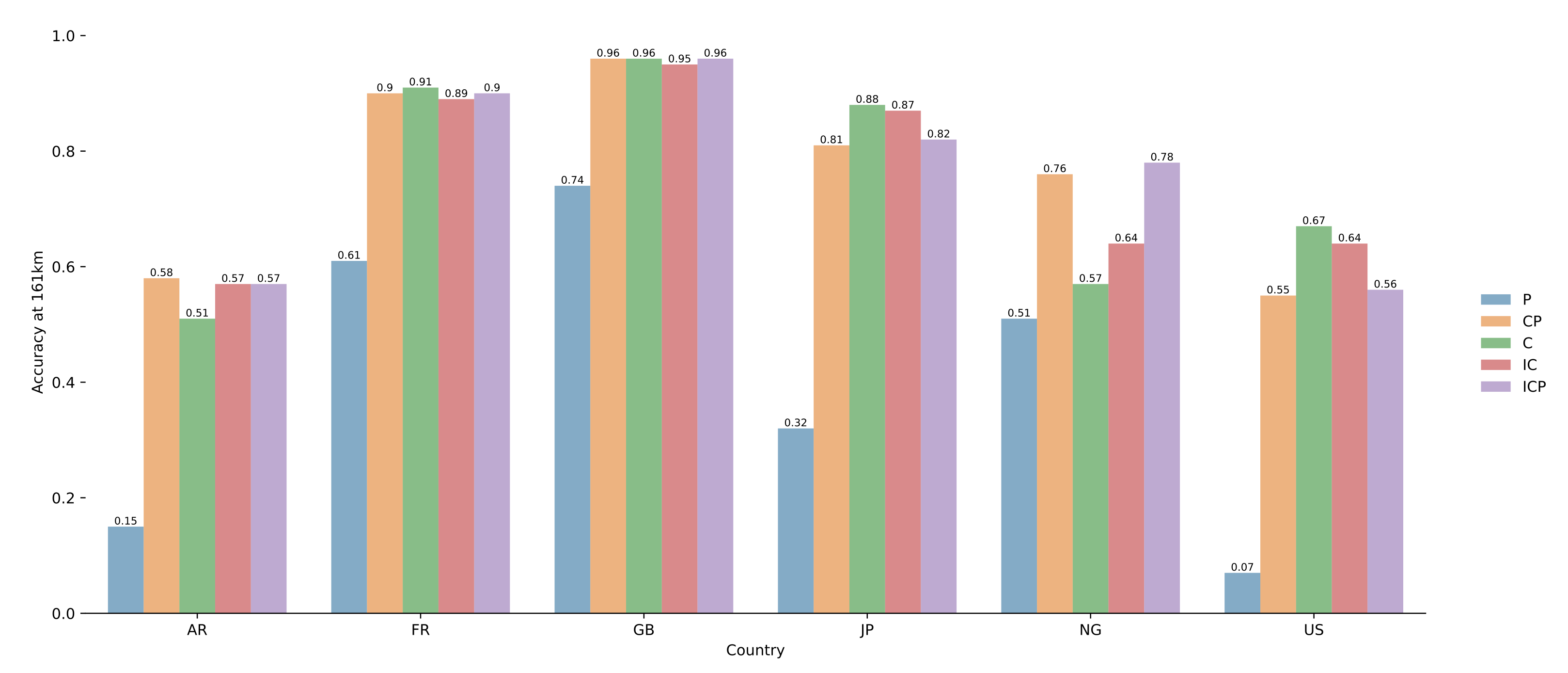
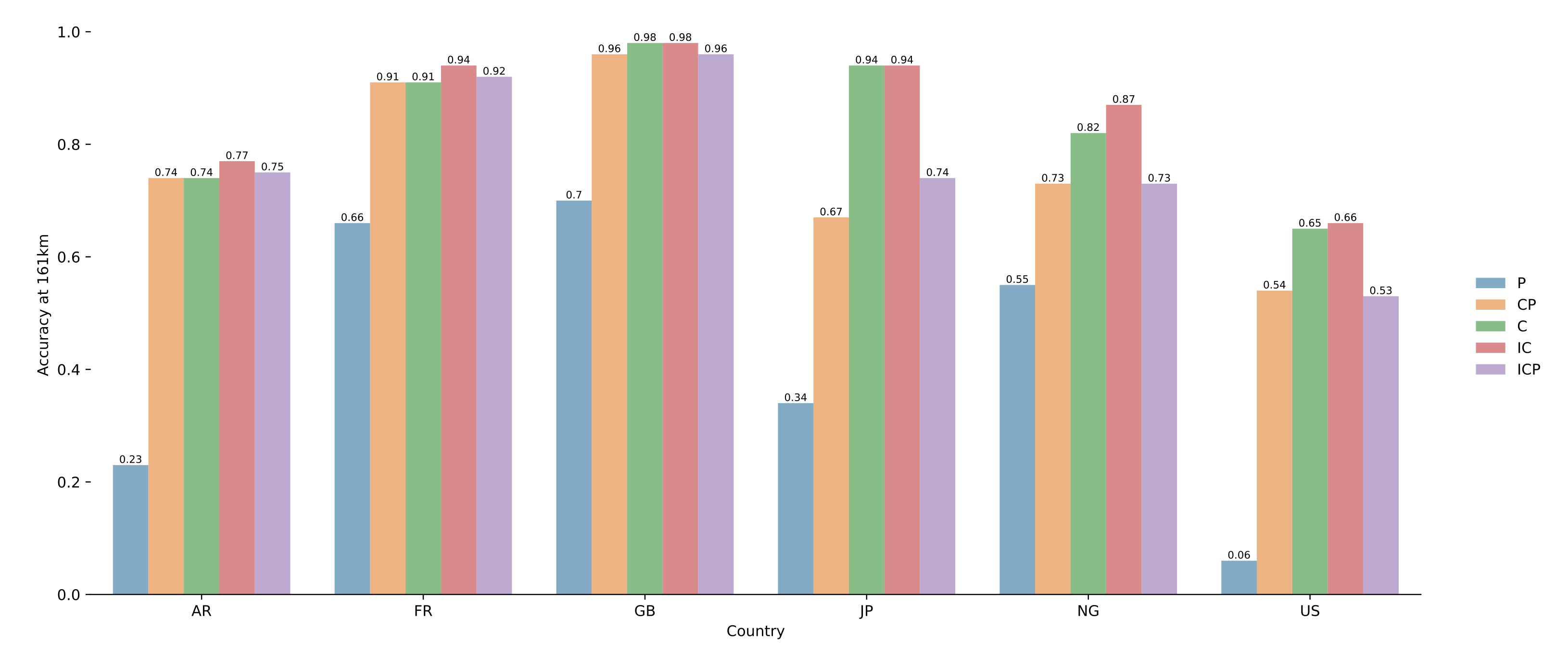
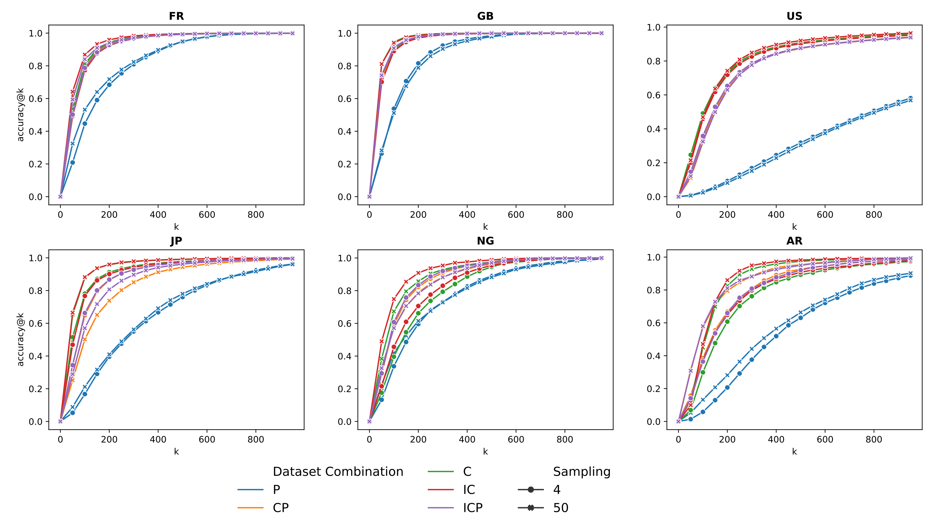
4.3. Results on Pairs of Toponyms

In a first experiment, we evaluate the geocoding accuracy of the model on pairs of toponyms. In order to replicate real-world requests on the model, we use pairs extracted from co-occurrences of places in Wikipedia. Figure 3 and Figure 4 show the results obtained considering different sampling strategies. Figure 5 shows the accuracy@k curve for each geographical scope, sampling, and dataset combination. We observe that models trained with pairs from the proximity-only dataset obtain the lowest accuracy. Furthermore, as shown on Figure 5, to obtain a high accuracy, the threshold value k needs to be high compared to other models. Focusing on the results obtained with a lower sampling (i.e., 4), our model shows high accuracies except for the US (Figure 3). Furthermore, models trained with only co-occurrences achieve the highest accuracies for some countries such as France (0.91), Great Britain (0.96), Japan (0.88), and the US (0.67). However, for countries like Argentina and Nigeria, co-occurrences are not enough and, for those, the addition of pairs from proximity and inclusion relationships increases the accuracy of the model. For instance, there is a 19% difference between the CP (co-occurrences + proximity) and C (co-occurrence only) models for Nigeria. We observe that pairs from proximity relationships increase the accuracy of some models, mostly for countries with less data. Table 1 highlights the difference between the number of co-occurrence pairs between France (376,088) and Nigeria (5638). A same observation can be made on the evolution of the loss value in Figure 6 where values for co-occurrence only model are higher than those for the other models with the combination of proximity and co-occurrences.

Figure 4 shows the results where models have been trained with pairs generated with a higher sampling. Most observations that were made with a lower sampling still apply. In terms of accuracy@k, co-occurrence pairs still give the best models. In addition, the increase of the number of pairs used in the training improves the model accuracy (France $0.91\to 0.94$, AR $0.58\to 0.77$, Nigeria $0.78\to 0.87$, Japan $0.88\to 0.94$, Great-Britain $0.96\to 0.98$.).

4.4. Geocoding Wikipages

In the per pair experiments, we evaluate the model in its ability to correctly geocode a toponym based on one pair (using another toponym as context). In real-world data, the number of context toponyms most of the times exceeds one. Thus, in this experiment, we evaluate the accuracy for geocoding a place using all the toponyms that appear in its Wikipedia page. To do that, we propose to use our model with the following simple heuristic: we predict the coordinates of every possible pair for a toponym $t_i\in T$ and the rest $C=\left\{(t_i,t_m)\right|t_m\in T-\left\{t_i\right\}\}$ appearing in the same context (i.e., the content of the Wikipedia page). Once the coordinates are recovered, we assign the coordinates $c_{t_i}$ following the next formula:

$$c_{t_i}=\{\frac{1}{\left|C\right|}\sum _{c\in \mathrm{coords}\left(\mathrm{C}\right)}{c}_{latitude},\frac{1}{\left|C\right|}\sum _{c\in \mathrm{coords}\left(\mathrm{C}\right)}{c}_{longitude}\},$$

where $\mathrm{coords}\left(\mathrm{C}\right)$ corresponds to coordinates returned by the model for each pair of C.

Figure 7 and Figure 8 show the results obtained with models trained with different sampling parameters. Figure 9 shows the accuracy@k curve for each geographical scope, sampling strategy, and dataset combination. Following the same trends as in the per pair geocoding experiments, with a sampling threshold value of 4, co-occurrence-only models obtain a high accuracy except for Nigeria and Argentina, where the addition of pairs from proximity and inclusion relationships improves the model accuracy. Unlike models trained with datasets with a lower sampling, a higher sampling causes the co-occurrence-only model to obtain the highest accuracy for every country, even Argentina and Nigeria. In a similar way, proximity-only trained models mostly obtain the lowest accuracy. As illustrated in Figure 9, these models only obtain high accuracies with a high value for k. Finally, there is no significant improvement in the highest accuracy between models trained with datasets with a different sampling.

4.5. Geocoding Results with Standard Corpora

In order to compare our model with other geocoding approaches, we evaluate also our model on geocoding datasets used in the literature. Here, we use SpatialML [34], TR-CONLL [35], the Lake District Corpus [36], and the War Of The Rebellion corpus [37].

Since our models are trained on pairs of toponyms from specific countries, the SpatialML and TR-CONNL datasets were divided by toponym country membership. Furthermore, there are no places located in Argentina or the United-States in SpatialML. Results are shown in

Table 2. Results obtained on state of the art corpora.

Dataset	Country	A@161	A@100	A@50	MDE	AUC
SpatialML	FR	0.36	0.33	0.33	304.86	0.77
	US	-	-	-	-	-
	JP	0.49	0.41	0.27	164.34	0.85
	AR	-	-	-	-	-
	NG	0.46	0.31	0.08	232.20	0.75
	GB	1.00	1.00	0.95	16.49	0.96
TR-CONLL	FR	0.28	0.28	0.23	317.17	0.72
	US	0.15	0.13	0.08	859.28	0.30
	JP	0.37	0.30	0.16	192.18	0.83
	AR	1.00	0.46	0.00	116.99	0.88
	NG	0.92	0.15	0.00	146.53	0.81
	GB	0.92	0.74	0.66	24.05	0.92
Lake District Corpus	GB	0.80	0.66	0.42	65.46	0.84
War of the Rebellion	US	0.11	0.05	0.02	603.17	0.38

. For the SpatialML dataset, we obtain high accuracies with places in Great-Britain but poor accuracies with toponyms from other countries. Concerning TR-CONLL, we obtain accurate predictions for toponyms from Argentina, Nigeria and Great Britain. For the Lake District Corpus, we also obtain an overall good accuracy. Finally, we obtain a very low accuracy for the War Of The Rebellion corpus as expected since our US model obtains the lowest scores. The fact that our models are trained on contemporary toponyms can also explain why we obtain lower accuracies. Like in the previous experiments, results obtained with the model trained on the United-State are weaker than in the other countries. In comparison, other methods succeed to obtain a 93% accuracy [37]. We investigate the reason of such low accuracies for the US in Section 5.4.

5. Discussion

This section presents summary discussion on the results...

5.1. Scalability

Neural network training can be time-consuming. Therefore, in this preliminary work, we trained different models on specific and controlled geographical areas. We only addressed the scalability issue by sampling pairs of toponyms generated with co-occurrences and proximity relationships. Concerning proximity, we decided to draw random pairs of toponyms in a specific region. As for co-occurrences, we decided to limit the number of pairs of toponyms extracted per article through a random selection process. Two issues arise from these choices. First, the proximity relation process is oversimplified, and a better extraction should lead to a significant impact of proximity in the model performance. Second, both selection processes allow duplicates, which may reduce the number of distinct pairs of toponyms.

5.2. Selection of Model Parameters

To analyse the impact of different parameter values, we compare the accuracy obtained on the France model by changing the n-gram size, the n-gram generation processes, and the number of LSTM sub-networks. Concerning the n-gram generation process, we compare other processes that split toponyms at the word level or by using the WordPiece algorithm used by BERT [38], which tokenizes a word into specific character n-grams known for their high occurrence in text.

Table 3. Impact of n-gram size, number of LSTM subnetwork, token split method (WP = Wordpiece, WL = word level)).

Parameter		LSTM		n-Gram
		1	2	2	3	4	5	6	WL	WP
Accuracy	@100 km	0.87	0.75	0.32	0.66	0.87	0.89	0.89	0.08	0.11
	@50 km	0.58	0.47	0.16	0.36	0.58	0.65	0.69	0.03	0.04
	@20 km	0.17	0.16	0.05	0.10	0.17	0.22	0.26	0.00	0.01

shows the results obtained by changing these different parameters. The results obtained with one LSTM sub-network correspond to a higher accuracy compared to a model with two LSTM sub-networks. Second, we observe that an increase of the size of the n-grams improve the model accuracy until 5-grams. Finally, the use of n-grams on the word level or generated with WordPiece lead to a worse accuracy.

5.3. Impact of Sampling

As the total number of toponym pairs for a country can be very high, we sample from all available pairs. Figure 10 shows the positive impact of a larger sampling for model training. For France and US, we only consider a sampling with k = 10 because of memory limits and the impact is thus limited. The impact is also limited for Great Britain, with only a small increase. For countries with less data, especially with less co-occurrences found on Wikipedia pages, the increase of the sampling has a high effect.

5.4. Why It Does Not Work for the US?

Our model trained with toponyms for different countries performs well except for the United States. In order to investigate this issue, we first produce prediction maps like the ones in Figure 11a,b. The aim is to reveal regions where our model performed well and where it has not. For producing these maps, we use the “per pair” experimental results and we associate each pair and its predicted coordinates with an hexagon cell using the H3 grid system. Finally, we compute, for each cell, the percentage of predictions that were correctly made (with a distance less than 161 km). Four countries covering the different types of results were selected: France, United States, Argentina and Japan. We observe in Figure 11a,d that predictions for pairs over France and Japan are mainly accurate, except for small areas (on the south west of France or the north of Japan). Places in these areas are sparse, which may explain the results. Figure 11b shows that for the US many areas are badly predicted by our model, mainly covering the West and South regions. Same as in France or Japan, places in these areas are more sparse. This is different from the North-East, where the model performed well around major US cities like New-York, Philadelphia, or Chicago. Therefore, one possible reason for the worse performance lies in place sparsity (at least in the dataset used in our tests). This is something we can also highlight for Argentina, as illustrated in Figure 11c.

Another lead lies in the referent ambiguity of toponyms for the selected countries. For quantifying the ambiguity of toponyms, we computed the average number of places for one toponym for each country. Results are shown in

Table 4. Average duplicates per toponym in Geonames.

Country	Average Number of Duplicates
FR	1.461936
GB	1.246243
AR	1.410444
NG	1.291725
US	1.640997
JP	1.286867

. If we compare France and the US, we can see that US toponyms belong to more places, but the difference seems not to be very significant and we will investigate further in future work.

6. Conclusions

In this article, we described an approach for geocoding toponyms using deep learning and character n-gram sequences. Our architecture is based on a neural network using LSTM cells to extract features for the character n-gram sequence. Our model requires two toponyms as input and returns latitude-longitude coordinates as output. The first toponym is the one to be geocoded, and the second is used as context to help the model resolve any reference ambiguity. We trained our model on six geographical areas and conduct three types of experiments for evaluation. The first evaluates the model efficiency for pairs of toponyms. The second evaluates the model efficiency for geocoding toponyms based on their Wikipedia webpages (using multiple pairs and a straight-forward heuristic). The third evaluates our model for geocoding standard datasets used in the literature. Results show high accuracy values in the first two experiments except for the US. They also shown that models trained with co-occurrences get the highest accuracies in most cases. However, when the country has a lower number of pages in Wikipedia, adding pairs generated from proximity and inclusion relationships enables us to increase the efficiency of the model.

For future work, we can consider the training and the development of a geocoding process that covers the entire world and not just one country. A second possibility for future work is to evaluate the potential of one such model with historical places, and assess the contribution of certain affixes in the geocoding.

References

1. Smith, D.A.; Crane, G. Disambiguating geographic names in a historical digital library. In Proceedings of the International Conference on Theory and Practice of Digital Libraries, Darmstadt, Germany, 4–9 September 2001; pp. 127–136. [Google Scholar]
2. Monteiro, B.R.; Davis, C.A., Jr.; Fonseca, F. A survey on the geographic scope of textual documents. Comput. Geosci. 2016, 96, 23–34. [Google Scholar] [CrossRef]
3. Buscaldi, D. Approaches to Disambiguating Toponyms. Sigspatial Spec. 2011, 3, 16–19. [Google Scholar] [CrossRef] [Green Version]
4. DeLozier, G.; Baldridge, J.; London, L. Gazetteer-Independent Toponym Resolution Using Geographic Word Profiles. In Proceedings of the 29th AAAI Conference on Artificial Intelligence, Austin, TX, USA, 25–30 January 2015. [Google Scholar]
5. Ardanuy, M.C.; Sporleder, C. Toponym disambiguation in historical documents using semantic and geographic features. In Proceedings of the 2nd International Conference on Digital Access to Textual Cultural Heritage, Göttingen, Germany, 1–2 June 2017; pp. 175–180. [Google Scholar]
6. Moncla, L.; McDonough, K.; Vigier, D.; Joliveau, T.; Brenon, A. Toponym disambiguation in historical documents using network analysis of qualitative relationships. In Proceedings of the 3rd ACM SIGSPATIAL International Workshop on Geospatial Humanities, Chicago, IL, USA, 5 November 2019; pp. 1–4. [Google Scholar]
7. Leidner, J.L. Toponym resolution in text: Annotation, evaluation and applications of spatial grounding. In ACM SIGIR Forum; ACM: New York, NY, USA, 2007; Volume 41, pp. 124–126. [Google Scholar]
8. Buscaldi, D.; Rosso, P. A conceptual density-based approach for the disambiguation of toponyms. Int. J. Geogr. Inf. Sci. 2008, 22, 301–313. [Google Scholar] [CrossRef]
9. Lieberman, M.D.; Samet, H.; Sankaranarayanan, J. Geotagging with local lexicons to build indexes for textually-specified spatial data. In Proceedings of the 26th International Conference on Data Engineering (ICDE), Long Beach, CA, USA, 1–6 March 2010; pp. 201–212. [Google Scholar]
10. Ester, M.; Kriegel, H.P.; Sander, J.; Xu, X. A Density-Based Algorithm for Discovering Clusters in Large Spatial Databases with Noise. In Proceedings of the 2nd International Conference on Knowledge Discovery and Data Mining KDD’96, Portland, OR, USA, 2–4 August 1996; pp. 226–231. [Google Scholar]
11. Moncla, L.; Renteria-Agualimpia, W.; Nogueras-Iso, J.; Gaio, M. Geocoding for texts with fine-grain toponyms: An experiment on a geoparsed hiking descriptions corpus. In Proceedings of the 22nd ACM SIGSPATIAL International Conference on Advances in Geographic Information Systems, Dallas, TX, USA, 4 November 2014; pp. 183–192. [Google Scholar]
12. Amitay, E.; Har’El, N.; Sivan, R.; Soffer, A. Web-a-where: Geotagging web content. In Proceedings of the 27th Annual International ACM SIGIR Conference on Research and Development in Information Retrieval, Sheffield, UK, 25–29 July 2004; pp. 273–280. [Google Scholar]
13. Overell, S.; Rüger, S. Using co-occurrence models for placename disambiguation. Int. J. Geogr. Inf. Sci. 2008, 22, 265–287. [Google Scholar] [CrossRef]
14. Batista, D.S.; Ferreira, J.D.; Couto, F.M.; Silva, M.J. Toponym disambiguation using ontology-based semantic similarity. In Proceedings of the International Conference on Computational Processing of the Portuguese Language, Coimbra, Portugal, 17–20 April 2012; pp. 179–185. [Google Scholar]
15. Hu, Y.H.; Ge, L. A Supervised Machine Learning Approach to Toponym Disambiguation. In The Geospatial Web: How Geobrowsers, Social Software and the Web 2.0 Are Shaping the Network Society; Scharl, A., Tochtermann, K., Eds.; Springer: London, UK, 2007; pp. 117–128. [Google Scholar]
16. Lieberman, M.D.; Samet, H. Adaptive Context Features for Toponym Resolution in Streaming News. In Proceedings of the 35th International ACM SIGIR Conference on Research and Development in Information Retrieval, Portland, OR, USA, 12–16 August 2012; pp. 731–740. [Google Scholar]
17. Molina-Villegas, A.; Muñiz-Sanchez, V.; Arreola-Trapala, J.; Alcántara, F. Geographic Named Entity Recognition and Disambiguation in Mexican News using word embeddings. Expert Syst. Appl. 2021, 176, 114855. [Google Scholar] [CrossRef]
18. Santos, J.; Anastácio, I.; Martins, B. Using machine learning methods for disambiguating place references in textual documents. GeoJournal 2015, 80, 375–392. [Google Scholar] [CrossRef]
19. Goldberg, Y. Neural network methods for natural language processing. Synth. Lect. Hum. Lang. Technol. 2017, 10, 1–309. [Google Scholar] [CrossRef]
20. Kamalloo, E.; Rafiei, D. A coherent unsupervised model for toponym resolution. In Proceedings of the 2018 World Wide Web Conference, Lyon, France, 23–27 April 2018; pp. 1287–1296. [Google Scholar]
21. Speriosu, M.; Baldridge, J. Text-driven toponym resolution using indirect supervision. In Proceedings of the 51st Annual Meeting of the Association for Computational Linguistics (Volume 1: Long Papers), Sofia, Bulgaria, 4–9 August 2013; pp. 1466–1476. [Google Scholar]
22. Gritta, M.; Pilehvar, M.T.; Limsopatham, N.; Collier, N. What is missing in geographical parsing? Lang. Resour. Eval. 2018, 52, 603–623. [Google Scholar] [CrossRef] [PubMed] [Green Version]
23. Cardoso, A.B.; Martins, B.; Estima, J. Using Recurrent Neural Networks for Toponym Resolution in Text. In Proceedings of the EPIA Conference on Artificial Intelligence, Vila Real, Portugal, 3–6 September 2019; pp. 769–780. [Google Scholar]
24. Kulkarni, S.; Jain, S.; Hosseini, M.; Baldridge, J.; Le, E.; Zhang, L. Multi-Level Gazetteer-Free Geocoding. In Proceedings of the International Combined Workshop on Spatial Language Understanding and Grounded Communication for Robotics, Bangkok, Thailand, 6 August 2021; pp. 79–88. [Google Scholar]
25. Peters, M.E.; Neumann, M.; Iyyer, M.; Gardner, M.; Clark, C.; Lee, K.; Zettlemoyer, L. Deep contextualized word representations. In Proceedings of the 2018 Conference of the North American Chapter of the Association for Computational Linguistics (NAACL), New Orleans, LA, USA, 1–6 June 2018. [Google Scholar]
26. Huang, Z.; Xu, W.; Yu, K. Bidirectional LSTM-CRF models for sequence tagging. arXiv 2015, arXiv:1508.01991. [Google Scholar]
27. Mikolov, T.; Chen, K.; Corrado, G.; Dean, J. Efficient Estimation of Word Representations in Vector Space. In Proceedings of the 1st International Conference on Learning Representations, ICLR Workshop Track Proceedings, Scottsdale, AZ, USA, 2–4 May 2013. [Google Scholar]
28. Akbik, A.; Bergmann, T.; Vollgraf, R. Pooled Contextualized Embeddings for Named Entity Recognition. In Proceedings of the 2019 Annual Conference of the North American Chapter of the Association for Computational Linguistics (NAACL), Minneapolis, MN, USA, 3–5 June 2019; pp. 724–728. [Google Scholar]
29. Agarap, A.F. Deep learning using rectified linear units (relu). arXiv 2018, arXiv:1803.08375. [Google Scholar]
30. Vrandečić, D.; Krötzsch, M. Wikidata: A Free Collaborative Knowledgebase. Commun. ACM 2014, 57, 78–85. [Google Scholar] [CrossRef]
31. Gorski, K.M.; Hivon, E.; Banday, A.J.; Wandelt, B.D.; Hansen, F.K.; Reinecke, M.; Bartelmann, M. HEALPix: A Framework for High-Resolution Discretization and Fast Analysis of Data Distributed on the Sphere. Astrophys. J. 2005, 622, 759–771. [Google Scholar] [CrossRef]
32. Cheng, Z.; Caverlee, J.; Lee, K. You are where you tweet: A content-based approach to geo-locating twitter users. In Proceedings of the 19th ACM International Conference on INFORMATION and Knowledge Management, Toronto, ON, Canada, 26–30 October 2010; pp. 759–768. [Google Scholar]
33. Jurgens, D.; Finethy, T.; McCorriston, J.; Xu, Y.T.; Ruths, D. Geolocation prediction in twitter using social networks: A critical analysis and review of current practice. In Proceedings of the Ninth International AAAI Conference on Web and Social Media, Oxford, UK, 26–29 May 2015. [Google Scholar]
34. Mani, I.; Hitzeman, J.; Richer, J.; Harris, D.; Quimby, R.; Wellner, B. SpatialML: Annotation Scheme, Corpora, and Tools. In Proceedings of the Sixth International Conference on Language Resources and Evaluation (LREC'08), Marrakech, Morocco, 28–30 May 2008. [Google Scholar]
35. Leidner, J.L. Toponym Resolution in Text: Annotation, Evaluation and Applications of Spatial Grounding of Place Names. Ph.D. Thesis, University of Edinburgh, Edinburgh, UK, 2007. [Google Scholar]
36. Rayson, P.; Reinhold, A.; Butler, J.; Donaldson, C.; Gregory, I.; Taylor, J. A deeply annotated testbed for geographical text analysis: The corpus of lake district writing. In Proceedings of the 1st ACM SIGSPATIAL Workshop on Geospatial Humanities, Redondo Beach, CA, USA, 7–10 November 2017; pp. 9–15. [Google Scholar]
37. DeLozier, G.; Wing, B.; Baldridge, J.; Nesbit, S. Creating a Novel Geolocation Corpus from Historical Texts. In Proceedings of the 10th Linguistic Annotation Workshop held in conjunction with ACL 2016 (LAW-X 2016), Berlin, Germany, 11 August 2016; pp. 188–198. [Google Scholar]
38. Devlin, J.; Chang, M.W.; Lee, K.; Toutanova, K. BERT: Pre-training of Deep Bidirectional Transformers for Language Understanding. arXiv 2019, arXiv:1810.04805. [Google Scholar]
Figure 1. Overview of our proposed deep neural network architecture.
Ijgi 10 00818 g001
Figure 2. Process of extracting Wikipedia co-occurrences extraction.
Ijgi 10 00818 g002
Figure 3. Geocoding accuracy per country and dataset combination with sampling = 4.
Ijgi 10 00818 g003
Figure 4. Geocoding accuracy per country and dataset combination with sampling = 50.
Ijgi 10 00818 g004
Figure 5. Evolution curve for geocoding accuracy@k.
Ijgi 10 00818 g005
Figure 6. Evolution of the loss value for the different models (sampling 50).
Ijgi 10 00818 g006
Figure 7. Accuracy for geocoding Wikipedia pages, per country and dataset combination with a sampling = 4.
Ijgi 10 00818 g007
Figure 8. Accuracy for geocoding Wikipedia pages, per country and dataset combination with a sampling = 50.
Ijgi 10 00818 g008
Figure 9. Accuracy@k evolution curve for geocoding Wikipedia pages.
Ijgi 10 00818 g009
Figure 10. Sampling Effect (PC).
Ijgi 10 00818 g010
Figure 11. Prediction maps for the results of our model.
Ijgi 10 00818 g011