Trajectory Similarity Analysis with the Weight of Direction and k-Neighborhood for AIS Data

Abstract

Automatic Identification System (AIS) data have been widely used in many fields, such as collision detection, navigation, and maritime traffic management. Similarity analysis is an important process for most AIS trajectory analysis topics. However, most traditional AIS trajectory similarity analysis methods calculate the distance between trajectory points, which requires complex and time-consuming calculations, often leading to substantial errors when processing AIS trajectory data characterized by substantial differences in length or uneven trajectory points. Therefore, we propose a cell-based similarity analysis method that combines the weight of the direction and k-neighborhood (WDN-SIM). This method quantifies the similarity between trajectories based on the degree of proximity and differences in motion direction. In terms of its effectiveness and efficiency, WDN-SIM outperformed seven traditional methods for trajectory similarity analysis. Particularly, WDN-SIM has a high robustness to noise and can distinguish the similarities between trajectories under complex situations, such as when there are opposing directions of motion, large differences in length, and uneven point distributions.

1. Introduction

Rapid developments in wireless communication technology and continuous improvements to positioning accuracy have led to significant progress in terms of the collection, analysis, and application of trajectory data. Trajectory data contains substantial information, which provides strong support for determining motion patterns and feature extraction. In the maritime transport field, the Automatic Identification System (AIS) is a new type of digital navigation aid system and maritime safety equipment that can record and transmit the position, heading, speed, and other information of a ship in real time [1,2]. AIS has a high spatiotemporal resolution, large data volumes, and covers the ports and seas in most global regions [3,4]. It has been used by an increasing number of studies to analyze various maritime traffic problems [5,6,7].

With the aid of cluster analysis, neural networks, association analysis, feature analysis, and other data mining technologies, massive quantities of AIS data can be analyzed to potentially extract useful rules from chaotic ship trajectory points [8,9,10,11,12]. This has important implications for various applications, including maritime safety [13,14], vessel destination prediction [15,16], collision risk identification [17,18], and maritime traffic management [19]. Among the currently popular ship trajectory analysis topics (e.g., trajectory classification, clustering, and trajectory anomaly detection, etc.), calculating the similarity between trajectories is one of the most important and basic processes [20,21,22]. As different data types or application scenarios require distinct similarity analysis methods, the trajectory similarity analysis method has a substantial impact on the accuracy of AIS ship trajectory data mining [20,23].

In the current research, the main similarity analysis methods used can be divided into warping-based methods (including Dynamic Time Warping (DTW), Longest Common Subsequence (LCSS), and Edit Distance on Real sequence (EDR), etc.) and shape-based methods (including the Hausdorff distance, One Way Distance (OWD), and the Fréchet distance, etc.) [24]. These methods and their extensions have promoted the research of AIS ship trajectory similarity analysis methods, widely used in maritime traffic. However, these traditional methods must calculate the distance between the sampling points, this calculation is complicated and is characterized by a substantial computational load. In particular, the message transmission frequency of AIS system is high, hence the trajectory points of ships are densely distributed, which consumes more computing time. Furthermore, due to the complicated maritime navigation conditions and the uncertain sampling interval, the sampling rate of most trajectories is uneven, which increases the distance between the trajectory points and affects the accuracy of the similarity results [25]. Therefore, Mariescu-Istodor et al. [26] proposed a faster and simpler method, referred to as Cell Similarity (C-SIM). C-SIM suggests that two trajectories are similar if they overlap upon expressing the trajectories on 2-D grid cells (Figure 1a shows the grid cell mapping method). C-SIM calculates the number of overlapping cells between the representative cell sequences of two trajectories, then divides it by the total number of cells to produce the similarity for the two trajectories. The authors also proposed Hierarchical Cell Similarity method (HC-SIM) [27], which optimized C-SIM at different zoom levels, extending the cell length to six levels (0.5%, 1%, 2%, 4%, 8%, and 16%). Calculations of the C-SIM measurement results are performed on each layer, taking the average value as the final result.

As an easily understandable and implementable method, C-SIM is based on the number of overlapping cells, thus avoiding the complicated distance calculation process. The computational load significantly decreases because the number of representative cells in the trajectory is usually less than the number of trajectory points. Most importantly, the use of grid cells instead of trajectory points reduces the impact that the distribution of sampling points has on the results, which addresses the issue of uneven sampling of ship trajectories. These are also the main reasons why we use cell sequences to represent trajectories in this study.

However, two challenges for similarity analyses of ship trajectories still remain. (1) The influence of diverse shipping directions on trajectory similarity is ignored. C-SIM only considers the spatial location of the track while ignoring the direction of movement. Two ships with similar routes may move in opposite directions which should not be treated as being similar trajectories. However, C-SIM fails to deal with this situation reasonably. (2) The equal and fixed importance of neighborhood cells does not adapt to complex analysis. C-SIM considers neighborhood cells and target cells to be equally important and fixed to eight neighborhoods. However, for tracks T₁, T₂, and T₃, as shown in Figure 1b, the similarity (T₁, T₂) = similarity (T₁, T₃) can be calculated. It is obvious that the distance between T₁ and T₂ is less than the distance between T₁ and T₃. Therefore, C-SIM is not suitable for analyzing trajectory similarity in the complex situation with high precision requirements.

To solve these two problems, we propose a cell-based similarity analysis method that combines the weight of the direction and k-neighborhood methods (WDN-SIM). Similar to C-SIM, WDN-SIM calculates the trajectory similarity based on the number of overlapping cells, but WDN-SIM additionally considers the movement direction relationship between two trajectories at the grid cell scale. Moreover, based on distance attenuation, WDN-SIM creates multi-level neighborhoods for the cells and sets different weights for neighborhoods at different levels. WDN-SIM also considers the overall characteristics of the trajectory and converts the similarity measurement result to the range of [−1, 1] to facilitate the comparison of similarity.

The remainder of this paper is organized as follows. Section 2 introduces the theoretical basis and principles of the WDN-SIM similarity analysis method. Section 3 presents a series of experiments to show the effectiveness and advantages of WDN-SIM. Section 4 discusses, in detail, the relevant parameters that affect the measurement results. Finally, Section 5 presents our conclusions and directions for future research.

2. Related Research

Researchers have recently developed many methods for trajectory similarity analyses. One of the most common methods is DTW [28], which obtains the cumulative distance between all optimally matched trajectory points through an iterative approach, thereby allowing the local expansion and contraction of the trajectory. DTW is widely used in AIS-related data analysis. For example, Li et al. [29] applied DTW to the robust ship trajectory clustering. Zhao et al. [30] improved DTW by considering the direction of trajectory point motion and the weight of endpoints. Liu et al. [31] combined DTW with the adaptive Douglas-Peucker (ADP) algorithm to improve the efficiency and accuracy of similarity measurements. However, the DTW method is sensitive to noise.

To overcome this noise sensitivity, Lachos et al. [32] combined the LCSS model with trajectory similarity measurements. The LCSS method quantifies the distance between 0 and 1. By setting a distance threshold, track point pairs, whose distance is less than the threshold, are added to the common trajectory sequence. The trajectory similarity is the distance for the longest common subsequence. LCSS has no strict requirements for the number of trajectory points or trajectory lengths and exhibits good robustness. However, the result is greatly affected by the distance threshold [33]. Furthermore, the EDR method was originally used to calculate the smallest number of operations (i.e., addition, deletion, and modification) required between two strings for complete consistency. This method has been widely used and was extended to similarity analyses of spatiotemporal trajectories [34,35,36,37,38]. However, similar to LCSS, this method cannot easily determine the distance threshold; LCSS and EDR only consider the similar or different components, respectively, such that the results of the similarity analysis are not ideal with uneven sampling point distributions or significant variations in the number of track points.

The methods mentioned above are all based on warping distance, but other studies have also proposed methods based on shape distance [24]. The Hausdorff distance method is a typical method based on shape distance. It calculates the maximum value of the shortest distance from a point on one trajectory to all points on the other trajectory. Wang et al. [39] found that the Hausdorff distance has an optimal effect when measuring the shape similarity between trajectories. However, as the Hausdorff distance must calculate the minimum value of the distance between a point and all points of the other trajectory, and does not consider the time sequence, the calculation efficiency is low and cannot identify the direction of motion. Therefore, Zhen et al. [22] proposed an improved Hausdorff distance method, which expresses the directional distance as the absolute value of the difference between the average course of two tracks. In some cases, this method can distinguish the trajectories of different motion directions but determining the weight of the directional distance remains difficult. Additionally, there are significant variations in the directions of movement when a ship moves at sea because of the influences of wind and seawater. Therefore, using the average direction of movement of all trajectory points as the direction of movement for the entire trajectory cannot yield the true direction of the ship at each point. Ma et al. [40] introduced OWD for the similarity calculation of ship trajectories when conducting research on ship motion pattern recognition. OWD calculates the average of all of shortest distances between two trajectory points [41]. OWD can reduce sensitivity to noise points, but still cannot identify the direction of movement.

Among shape-based methods, another commonly used technique is the Fréchet distance, which originates from the problem associated with the shortest leash length required when walking a dog, i.e., the shortest distance required for the intersection of two curves. Therefore, unlike the Hausdorff distance and OWD, the Fréchet distance considers the time relationship between the trajectory points, such that the resulting trajectories in the same and opposite directions are highly different [42,43,44]. However, as the distance between curves is difficult to obtain, the discrete Fréchet distance is now more commonly used, i.e., calculating the maximum value of the minimum distance between discrete point pairs [45,46].

3. Methodology

3.1. Overall Idea

The method proposed in this study divides the 2-D space where the trajectory is located into regular grids while combining the spatial neighborhood and direction of the trajectory to analyze the similarity between trajectories. Figure 2 shows the process of this method, which was divided into three steps.

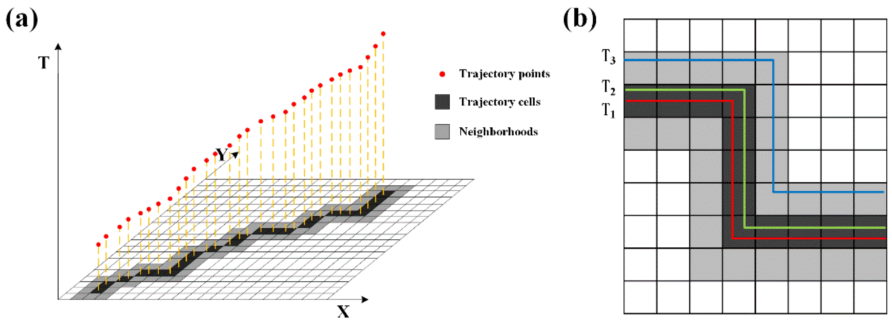
• Reconstruct the representative trajectory. Based on the Maritime Mobile Service Identity (MMSI) code, navigation state, and time interval of the trajectory point, we extracted the trajectory segment. The trajectory segment was then mapped to the corresponding grid cells according to its spatial position. The constructed cell sequence was used to calculate the trajectory similarity.
• Quantify the direction and neighborhood of the trajectory. We assigned corresponding weights to various directional relationships for different trajectories on the same grid cell. The directional relationships included three types: same direction, inclined direction, and opposite direction. Meanwhile, different neighborhoods of the central cells were also given corresponding weights according to the degree of proximity to the central cell.
• Calculate similarity between trajectories. The similarity between the trajectories was measured by calculating the number and proportion of overlapping cells between representative trajectories, followed by assigning corresponding weights to the k-neighborhood and motion direction characteristics.

3.2. Reconstructing the Representative Trajectory Based on Cell

A ship trajectory is a set of points arranged in chronological order by a series of trajectory points with time labels [23], which can be expressed as $\mathrm{P}=\left({\mathrm{p}}_1,{\mathrm{p}}_2,{\mathrm{p}}_3,{\mathrm{p}}_4,\dots ,{\mathrm{p}}_n\right)$, where n is the number of track points in a certain track and ${\mathrm{p}}_n$ is the nth track point present in an AIS record. The attributes of an AIS record include the ship name, call sign, International Maritime Organization (IMO) code, MMSI code, ship type, navigation status, length, width, draft, heading, course, speed, longitude, latitude, destination, estimated time of arrival, and time. The track points for different ships can usually be identified by their unique MMSI code [47]. Reconstructing a representative trajectory mainly includes two steps: trajectory identification and trajectory point mapping.

Trajectory segment identification. Owing to the large time intervals in AIS data, the AIS data for a ship includes all previous voyage information. After obtaining the AIS record of each ship, identifying the records for different voyages is thus necessary. We identified the stopping points in the trajectories to separate different trajectory segments. First, we sorted all trajectory points belonging to the same ship in chronological order, then divided the trajectory points of that ship into sailing and stopping points. The stopping points included situations where the navigation status was docking, anchoring, loading or unloading cargo, stranded, or maintenance, etc., which indicated that either the ship has ceased operation or that the time interval between one point and the following track point exceeds 12 h. The sailing points describe the condition when a ship operates normally at sea. Based on the above rules, we divided the trajectory points of ships into different trajectories according to the positions of stopping points. Figure 3 illustrates a diagram of trajectory identification based on stopping points. As shown in Figure 3b, when a stopping point appears, the original trajectory is divided into two new trajectories by the stopping point. Figure 3a shows multiple consecutive stopping points, in which the first stopping point is the end of the previous trajectory and the last stopping point is the starting point of the next trajectory.

When gridding the trajectory, we used a square structure. Storing and indexing was convenient because the division method for the square grid was more consistent with the latitudinal and longitudinal axes. In contrast, as our method required the calculation of all cells within a certain range surrounding the central cell, the square neighborhood divided the cell into more layers within a smaller distance.

For trajectory point mapping, the speed of the ship usually varied; due to unstable signals at sea, trajectory points were often missing. Simply assigning the attributes of all trajectory points to the grid cells when mapping the trajectory points would produce a trajectory with multiple moving directions in the same cell or interruptions in the constructed representative trajectory. To solve these problems, we set the following rules. (1) As shown in Figure 4a, when a trajectory had consecutive trajectory points passing through the same cell, the average value of the directions of these trajectory points was taken as the direction of the entire trajectory on the cell. (2) As shown in Figure 4b, when the representative trajectory was interrupted, the last trajectory point before the interruption (d₆) and the first trajectory point after the interruption (d₇) form a line, the cell passing through the midpoint of the line was added to the representative trajectory. The average value of the directions of d₆ and d₇ was used as the movement direction in cells with missing information, until there was no interruption in the trajectory.

3.3. Weight of Direction and Neighbor Cell

In this section, we introduce the method for measuring the direction relations and neighborhoods, which is not considered in C-SIM; however, these are important factors that affect the results of ship trajectory similarity measurements. As we calculated the similarity between the trajectories based on the number of overlapping cells, we quantified the relationship between the direction of motion between two trajectories in overlapping cells and the different levels of neighborhoods for each cell. This was then added to the final similarity calculation function in the form of a weight.

3.3.1. Weight of Direction

As the course of each point was recorded in the AIS data, we used it to indicate the direction of the track point. We used the average course for all points in the same cell as the trajectory direction in the cell. To obtain the movement direction relationship of two trajectories for each overlapping cell, we used the absolute value of subtracting their directions in the cell, as represented by Ɵ (Ɵ ∈ [0°, 180°]). The larger the value of Ɵ, the greater the difference in direction.

To avoid excessive interference from the direction, as the direction of ship movement was unstable, we simplified the directional relationship between the trajectories into the following three relationships: same direction, inclined direction, or opposite direction. We divided Ɵ at equal intervals, using 60° as the boundary, to allocate equal proportions to the three relations. (1) The same direction, with a Ɵ range of [0°, 60°], represents the highest directional similarity, such that the highest weight of 1 was assigned. (2) The inclined direction, with a Ɵ range of (60°, 120°], represents a relatively high direction similarity, such that the weight of 0.5 was assigned. (3) The opposite direction, with a Ɵ range of (120°, 180°], represents the lowest direction similarity, such that the lowest weight of −1 was assigned. The weight was set to a negative value because an opposite directional relationship weakens the overall similarity. The mathematical expression is as follows:

$$\{\begin{array}{c}{w}_D^1=1, \mathrm{if} \mathsf{Ɵ}\in \left[0°,60°\right]\\ w_D^2=0.5, \mathrm{if} \mathsf{Ɵ}\in \left(60°, 120°\right]\\ w_D^3=-1, \mathrm{if} \mathsf{Ɵ}\in \left(120°, 180°\right]\end{array},$$

(1)

where $w_D^1$, $w_D^2$, and $w_D^3$ are the weights corresponding to different directional relationships between the trajectories.

3.3.2. Weight of Neighbor Cells

As the distance increases, the degree of similarity between the trajectories slowly decreases, but due to the arbitrary division of grid cells, adjacent points may be assigned to different cells, which makes the similarity directly change from 1 (same) to 0 (completely different). Therefore, to fully consider the influence of the spatial relationship between trajectories and improve the rationality of the similarity measurement, we added the k-neighborhood of the trajectory grid cell, where k is the maximum number of neighborhoods that participate in the calculation. We set different weight values for neighborhoods at different distances for smoother change in similarity. Figure 5a shows the division method, where “a” is the central cell to which the neighborhood belongs and the remaining cells of the same color represent the same level of neighborhood for “a”. The number in the cell corresponds to the level of the neighborhood: cell 1 is the nearest neighbor domain for central cell and cell 2 is the second nearest neighbor domain, extending outward in turn. The number of neighborhood levels involved in the calculation can be determined based on the size of the study area and the density of the trajectory points.

To determine the weights of neighborhoods at different levels, as a greater distance between cells results in a lower similarity, we introduced Inverse Distance Weighted method (IDW). We used different neighborhood levels as “distances” and the largest neighborhood level k participating in the calculation as the “distance threshold” to assign corresponding weights to the neighborhoods of each level. The higher the neighborhood level, the smaller the weight. This method can be expressed as follows:

$$w_N^k=\frac{1}{{\left(k+1\right)}^{0.5}} ,$$

(2)

where $w_N^k$ is the weight of the k-neighborhood and k is the level of the neighborhood. According to the above formula, the weights of 1–5 levels are 0.707, 0.577, 0.500, 0.447, 0.408, respectively.

3.4. Measuring Similarity between Trajectories

The key to trajectory similarity analysis is the determination of the distance. We used the number of overlapping cells between representative trajectories as the “trajectory distance”, assigning corresponding weights to different movement direction relationships and neighborhood levels for each overlapping cell (see Section 3.3 for the weight calculation rules). The calculations for this method included two steps: (1) calculate the degree of overlap between two cell sequences and (2) calculate the proportion of the overlapping part of the trajectories in the total length. Finally, we multiplied the results of these two steps.

When calculating the degree of overlap, to make the similarity calculation results more comparable, we divided the number of overlapping cells, considering the weight of the direction and neighborhood, by the total number of overlapping cells. This result was converted to the range of [−1, 1], where 1 indicates that the two trajectories were identical and in the same direction, −1 indicates that the two trajectories were identical and in opposite directions, and 0 indicates that the two trajectories were irrelevant; the closer the result is to 0, the lower the degree of similarity.

When the total number of cells in the trajectories was identical, if the ratio of overlapping cells in the two trajectories to the total cells was high, the similarity between them was also high. Therefore, we considered the proportion of the overlapping part of the trajectories to the total length. This is achieved by calculating the ratio of the number of overlapping cells to the total number of cells in the two trajectories, where the similarity was expressed as follows:

$$S=\frac{{{\displaystyle \sum }}_{i=1,j=0}^{n,k}{w}_N^j\left(w_D^1{c}_1^{ij}+w_D^2{c}_2^{ij}+w_D^3{c}_3^{ij}\right)}{{{\displaystyle \sum }}_{i=1,j=0}^{n,k}\left(c_1^{ij}+c_2^{ij}+c_3^{ij}\right)}\ast \frac{C_{overlap}}{C_{all}},$$

(3)

where $S$ is the similarity for the two trajectories involved in the calculation; $i$ is the $i^{th}$ overlapping cell between the trajectories; $n$ is the total number of overlapping cells between the trajectories; $w_N^j$ is the weight of the j-neighborhood and $j$ is the level of the neighborhood; $w_D^1$, $w_D^2$, and $w_D^3$ are the weights corresponding to different directional relationships between the trajectories; $c_1^{ij}$ is the number of motion directions at the same interval in the j-neighborhood of the $i^{th}$ overlapping cell between the two trajectories; $c_2^{ij}$ is the number of motion directions in adjacent intervals to the j-neighborhood of the $i^{th}$ overlapping cell between the two trajectories; $c_3^{ij}$ is the number of motion directions in opposite intervals in the j-neighborhood of the $i^{th}$ overlapping cell between the two trajectories; $C_{all}$ is the total number of cells in the two trajectories; and $C_{overlap}$ is the number of overlapping cells.

4. Performance Evaluation

4.1. Experimental Design

4.1.1. Experimental Dataset

The dataset used in this study was AIS data purchased from the Shipping News Network of Elane, Inc. The collection period was from 1 to 7 January 2015, and the range was 94° E–127° E and 6° S–26° N. We first processed the data and deleted records with incorrect MMSI codes, incomplete attributes, and repeated records [3]. The ship type was then set to cargo. The data used in experiments to quantitatively analyze the effectiveness and efficiency of the WDN-SIM method were selected from this AIS dataset.

4.1.2. Trajectory Similarity of Different Positional Relationships

The experiment designed herein verified the rationality of the proposed method (WDN-SIM) by evaluating the calculated similarity results between the trajectories of different position relationships in real application scenarios. As WDN-SIM can distinguish whether the trajectory movement direction is the same or opposite, this experiment specifically compared the two cases. Furthermore, this experiment compared and analyzed the similarity of different parts of a trajectory to compare the calculation results of different position relationships using the proposed method. Figure 6 shows the trajectory data selected for this experiment, where Trajectories 1, 2, and 3 had 324, 265, and 310 trajectory points, respectively, and the average sampling interval was approximately 500 m; the direction of movement between trajectories 1 and 2 was the same, while the direction of movement between trajectories 1 and 3, and between trajectories 2 and 3 were opposite; A, B, and C were the further divided areas; the arrows represented the direction of movement of the trajectory.

4.1.3. Comparisons with Other Similarity Measurement Methods

In this section, we used four trajectory transformation experiments and compared the proposed method (WDN-SIM) with several typical ship trajectory similarity measurement methods to verify the effectiveness and efficiency of WDN-SIM [21,48]. The methods used for comparison included DTW, EDR, LCSS, the Fréchet distance, the Hausdorff distance, OWD, and HC-SIM.

Parameter Settings. The parameters involved in the WDN-SIM method included the cell length (L) and maximum neighborhood level (k). By achieving an optimal balance between the trajectory compression rate and feature point retention, after numerous comparison experiments, we set L and k as 2 km and 2, respectively (please see Section 4 for a detailed discussion on the methods of parameter setting and their influence on the results). To maintain consistency, the distance threshold of the LCSS and EDR was correspondingly set as 2 km. After testing, we found that grid cell sizes ≥ 24 km yielded similarity results with negligible changes, so the minimum cell length of HC-SIM was set to 0.75 km. Unless explicitly stated, the parameters in all experiments were set to the above values (

Table 1. Parameter settings of different methods.

Parameter (km)	LCSS	EDR	HC-SIM	WDN-SIM
Distance threshold (km)	2	2	- 1	-
Minimum cell length (km)	-	-	0.75	-
Cell length (L) (km)	-	-	-	2
Maximum neighborhood level (k)	-	-	-	2

¹—indicates that the method does not require to set the corresponding parameters.

).

Additionally, except for WDN-SIM and HC-SIM, several other methods required the calculation of distances. Haversine is a formula that obtains the arc distance between two points on longitude and latitude; this method can approximate the shortest distance between points on the surface of Earth [49], allowing the measurement of distance as follows:

$$d=2r\ast {\sin }^{-1}\sqrt{{\sin }^2\left(\frac{\Delta Lat}{2}\right)+\cos \left(La{t}_1\right)\ast \cos \left(La{t}_2\right)\ast {\sin }^2\left(\frac{\Delta Lon}{2}\right)},$$

(4)

where $d$ is the Haversine distance between two points; $r$ is the approximate radius of Earth (6371 km); $\Delta Lat$ denotes subtraction between the latitudes of two points; $\Delta Lon$ denotes subtraction between the longitudes of two points; and $La{t}_1$ and $La{t}_2$ are the latitudes of the two points, respectively.

Effectiveness. Our experiments used 20 adjacent trajectory pairs in different regions from the AIS dataset, taking the average value as the final result. The average number of points for each trajectory was 350, and the sampling interval was about 500 m. The effectiveness of WDN-SIM was tested by comparing the measured results of the different methods in various transformations (including changing sampling, adding noise, changing direction, and deleting endpoints). Owing to the lack of benchmarks for the similarity of two trajectories, the measurement results for the various methods had different ranges of value and significance; for example, LCSS, EDR, HC-SIM, and WDN-SIM obtained comparable degrees of similarity, whereas DTW, Fréchet, Hausdorff, and OWD only calculated the distance, such that we applied the change rate in the results for comparison:

$$R=\frac{\left|r^{\prime }-r\right|}{r}\ast 100,$$

(5)

where $R$ is the change rate of similarity measurement result, $r$ is the result before a change, and $r^{\prime }$ is the result after a change.

The four types of transformations methods applied in this study are described in detail as follows.

Changing sampling rate. It includes two types: increasing sampling rate and decreasing sampling rate. Increasing sampling rate was achieved by randomly adding the midpoint, $p_m$, of two continuous sampling points, $p_i$ and $p_{i+1}$, where the coordinates, time, speed, and course of $p_m$ were the mean of $p_i$ and $p_{i+1}$. Decreasing sampling rate was achieved by randomly deleting a portion of trajectory points from the original trajectory. In this experiment, the sampling rate range was set to 50–150%, where the robustness of the method to a change in sampling rate was evaluated by comparing the changing rate of the measurement result. Additionally, to avoid deleting important points and causing large errors, we used the Threshold-guided Sampling method, proposed by Zhang et al. [50], to extract feature points. The feature points of the trajectory were not changed when adding or deleting points. The specific method was as follows. First, the trajectory points in a trajectory were sorted in chronological order. Changes in the speed between two continuous trajectory points were then calculated, in addition to the course. Finally, based on experience, trajectory points with direction changes > 5° or speed changes > 2 knots were set as feature points.

Adding noise. Noise points were added by randomly moving 1–10% of the original trajectory points in the range of 2–10 km. The change rate reflected the sensitivity of different methods to noise points.

Changing direction. In this experiment, we rotated one of the two trajectories moving in the same direction by 90° and 180°, where the direction of rotation was clockwise and the center of rotation was the midpoint of the trajectory. The course was also increased by 90° and 180°, such that the movement direction relationship between the trajectories after rotation became vertical and reverse, respectively. By comparing the similarity measurement results before and after the transformations, we tested the recognition ability of the different methods with respect to the three movement direction types.

Deleting endpoints. We deleted 5–20% of the points from one end of a trajectory; the resulting change rate was used to measure the ability of the method to identify the length differences between trajectories.

To sum up, during the experiment of changing sampling rate or adding noise, if the change rate after transformation was smaller, the method was less affected by such transformation, hence the stability was higher. However, during the experiment of deleting endpoints, if the change rate after transformation was smaller, the ability to recognize similarities between trajectories of different lengths was weaker.

Finally, we measured the similarity of trajectory pairs containing different numbers of trajectory points. The efficiency of the method was evaluated by comparing the time required for each method to obtain the similarity between two trajectories.

4.2. Results and Analysis

4.2.1. Results of Different Positional Relationship Experiments

Figure 7a–c shows the experimental results between trajectories 1 and 2, 2 and 3, and 1 and 3. Figure 7 suggests that the similarity between trajectories 1 and 2 was the largest and positive, indicating that the similarity between trajectories 1 and 2 was the highest and the movement direction was identical overall. The similarity results of trajectories 3 and 1, and 3 and 2 were negative because the movement directions between the two trajectories were opposite. The results show that the WDN-SIM method can distinguish the similarity between trajectories with the same and opposite movement directions based on the positive and negative values of the measurement results. From the results of each part, the proximity of different parts between the trajectories was different and the similarity results were also different. From the similarity measurement result of trajectories 2 and 3 in part A (Figure 7b), the similarity between the mutually perpendicular trajectories tended to be 0. Comparing the similarity results in part B between each trajectory pair, the closer the trajectories, the greater the absolute value of the similarity results. In part C, the three trajectories were the closest to each other and the similarity result value was also the highest. The results indicate that WDN-SIM can sufficiently distinguish the similarities between trajectories with different spatial relationships.

4.2.2. Results of Measurement Comparison Experiments

Figure 8 shows the result of the experiment when changing the sampling rate. WDN-SIM was less affected by the sampling rate because the neighborhood cell had a buffering effect; the cells were filled even when the cells were interrupted. Among other methods, DTW was the most sensitive to changes in the sampling rate because it needed to match all trajectory points when calculating the distance, such that changes in the number of points and distance had a significant effect on the results of this method.

As shown in Figure 9, DTW remained the most sensitive to added noise points. OWD was the least sensitive to noise points because it used the mean of the minimum distance; the change in the distance caused by a small number of noise points was weakened by the other tracking points. The other methods were not sensitive to the added noise points.

Table 2. Results of experiment with a changing direction.

Direction	DTW 1	EDR	LCSS	Fréchet 1	Hausdorff 1	OWD 1	HC-SIM	WDN-SIM
Same	1468.933	0.593	0.652	38.764	36.379	4.580	0.785	0.479
Perpendicular	22,980.964	0.012	0.014	142.549	97.059	51.139	0.112	0.005
Opposite	30,262.603	0.009	0.014	197.429	36.379	4.577	0.787	−0.453

¹ Units for the DTW, Fréchet, Hausdorff, and OWD methods are km.

lists the result of the experiment with changing directions. WDN-SIM identified the similarity of trajectories with the same, perpendicular, and opposite directions, which allowed finer classification and clustering. For trajectories with the same and opposite directions, the similarity can be distinguished by the positive and negative values of measurement results. For trajectories with the same and perpendicular directions, the similarity can be distinguished by the value of the measurement result. The Hausdorff, OWD, and HC-SIM methods could not distinguish the similarity of trajectories in the same and opposite directions. DTW, EDR, LCSS, Fréchet, and WDN-SIM could not distinguish the similarity of trajectories with vertical and opposite directions. Among the methods of comparison, WDN-SIM was the only method that could distinguish the three directional relationships.

As shown in Figure 10, for two similar trajectories, when the length of one changed, the DTW, OWD, and WDN-SIM methods showed higher acuity than the other methods, indicating that these methods were better at identifying differences in the trajectory length.

As shown in Figure 11, when the trajectory had a small number of points, WDN-SIM was less efficient than other methods, mainly because WDN-SIM searched for cell neighborhoods, and was thus time-consuming. However, when there were many trajectory points, WDN-SIM was more efficient than other methods because they required traversing the trajectory points multiple times. For distance-based methods, more trajectory points require a longer calculation time. Cell-based methods did not require measuring the distance, such that HC-SIM and WDN-SIM were less affected by the increase in the number of trajectory points. Moreover, because HC-SIM needed to calculate the average of the similarity of six different cell lengths, its efficiency was lower than that of WDN-SIM.

5. Discussion

5.1. Grid Cell Size Selection Problem

The proposed method extracted the representative trajectory by mapping the trajectory points on a regular grid cell. Different cell sizes have a significant impact on the accuracy of trajectory extraction results. If the cell size is too large, the trajectory is excessively compressed and key features are blurred. In contrast, an excessively small grid cell size increases the number of cells in the representative trajectory and increases the computational load. Therefore, this section designed an experiment to find the optimal cell size. Specifically, as the selection of the cell size is mainly related to the shape and distribution density of the trajectory, we set different cell sizes to compare the relationship between the trajectory point compression rate and the feature point missing rate. We used the Threshold-guided Sampling method (discussed in Section 4.1.3) to extract the feature points of the trajectory [50]. Additionally, we used cell length to reflect the grid cell size. Based on

Table 3. Results of the trajectory point compression rate and the feature point missing rate for different cell lengths.

	Cell Length (km)
	1	2	3	4	5
Trajectory point compression rate (%)	28	71	76	82	87
Feature point missing rate (%)	3	10	17	29	38

, for the experimental data in this study, when the cell length was set to 2 km, the two indices reached an optimal balance.

5.2. k Setting Problem

To illustrate the influence that the k value has on the results of the similarity measurement, the following comparative experiment was conducted. We chose six adjacent trajectories moving in the same direction for the experiment (as shown in Figure 12). The change in the similarity measurement results was then compared for different k values. To compare the results, a certain trajectory was used as the target trajectory. Figure 12 shows the similarity results between the target trajectory and other trajectories, where the horizontal axis is arranged in descending order according to the degree of proximity. Overall, when considering the neighborhood, the value of the similarity measurement result was significantly increased, while the order of proximity remained unchanged. According to the results between trajectories 1 and 3, 1 and 4, and 3 and 5, some trajectory pairs that did not have a similar relationship when not considering the neighborhood, exhibited low similarity when considering the neighborhood. This shows that using neighbor cells can expand the range of the trajectory similarity comparison. However, the more neighborhood levels considered, the longer the execution time required by the program. Therefore, the running time must be considered when determining the k value. We also note that when k = 2, the neighbor grid involved in the calculation was exactly equivalent to the eight neighborhoods of the central cell, therefore, the diagonal cell was not ignored. Based on the above analysis, k was generally set as 2.

6. Conclusions

We proposed a similarity analysis method for AIS ship trajectories in this study, referred to as WDN-SIM, which addresses the problem of C-SIM, which cannot identify the trajectory direction and yields an unreasonable neighborhood weight. WDN-SIM was compared with several traditional trajectory similarity analysis methods (i.e., DTW, EDR, LCSS, discrete Fréchet distance, Hausdorff distance, OWD, and HC-SIM), which showed that WDN-SIM was comparatively less affected by the trajectory sampling rate and noise points, could identify trajectories of different lengths, and performed well in terms of the efficiency, so WDN-SIM is suitable for the similarity analyses of AIS data.

WDN-SIM can not only recognize the similarity between trajectories with different motion direction relationships, but it can also obtain entirely different similarity results for trajectories with the same, perpendicular, and opposite directions. Existing methods can only identify two of these relationships. Therefore, WDN-SIM can obtain more finely resolved trajectory similarity results, which can improve the accuracy of subsequent trajectory classifications and clustering analyses. Additionally, the similarity results obtained with WDN-SIM ranged from −1 to 1. A fixed range such as this can improve the comparability of the results.

WDN-SIM provides new insights for improving the methods used to quantify the similarities between different ship trajectories. This is important in terms of logistics, shipping efficiency, and course plotting, among other issues, in addition to facilitating trajectory analyses, such as clustering, classification, or anomaly detection. To generalize the proposed method, our future research needs to explore the spatio-temporal similarities in AIS trajectories. In addition, since we judge the movement direction of the trajectory in each grid cell by calculating the average value of the direction, the direction will be inaccurate for complex situations such as zigzag movement or circular movement. Thus, further research should investigate the direction recognition method in complex scenes.

References

1. Metcalfe, K.; Bréheret, N.; Chauvet, E.; Collins, T.; Curran, B.K.; Parnell, R.J.; Turner, R.A.; Witt, M.J.; Godley, B.J. Using satellite AIS to improve our understanding of shipping and fill gaps in ocean observation data to support marine spatial planning. J. Appl. Ecol. 2018, 55, 1834–1845. [Google Scholar] [CrossRef]
2. Yan, Z.; Xiao, Y.; Cheng, L.; Chen, S.; Zhou, X.; Ruan, X.; Li, M.C.; He, R.; Ran, B. Analysis of global marine oil trade based on automatic identification system (AIS) data. J. Transp. Geogr. 2020, 83, 102637. [Google Scholar] [CrossRef]
3. Cheng, L.; Yan, Z.J.; Xiao, Y.J.; Chen, Y.M.; Zhang, F.L.; Li, M.C. Using big data to track marine oil transportation along the 21st-century maritime silk road. Sci. China Technol. Sci. 2019, 62, 677–686. [Google Scholar] [CrossRef]
4. Feng, M.; Shaw, S.L.; Peng, G.; Fang, Z. Time efficiency assessment of ship movements in maritime ports: A case study of two ports based on AIS data. J. Transp. Geogr. 2020, 86, 102741. [Google Scholar] [CrossRef]
5. Mou, N.; Ren, H.; Zheng, Y.; Chen, J.; Niu, J.; Yang, T.; Zhang, L.; Liu, F. Traffic Inequality and Relations in Maritime Silk Road: A Network Flow Analysis. ISPRS Int. J. Geo-Inf. 2021, 10, 40. [Google Scholar] [CrossRef]
6. Riveiro, M.; Pallotta, G.; Vespe, M. Maritime anomaly detection: A review. Wiley Interdiscip. Rev. Data Min. Knowl. Discov. 2018, 8, e1266. [Google Scholar] [CrossRef] [Green Version]
7. Zhao, L.; Shi, G. A trajectory clustering method based on Douglas-Peucker compression and density for marine traffic pattern recognition. Ocean Eng. 2019, 172, 456–467. [Google Scholar] [CrossRef]
8. Zhao, L.; Shi, G. Maritime Anomaly Detection using Density-based Clustering and Recurrent Neural Network. J. Navig. 2019, 72, 894–916. [Google Scholar] [CrossRef]
9. Chen, R.; Chen, M.; Li, W.; Wang, J.; Yao, X. Mobility Modes Awareness from Trajectories Based on Clustering and a Convolutional Neural Network. ISPRS Int. J. Geo-Inf. 2019, 8, 208. [Google Scholar] [CrossRef] [Green Version]
10. Mascaro, S.; Nicholson, A.; Korb, K. Anomaly detection in vessel tracks using Bayesian networks. Int. J. Approx. Reason. 2014, 55, 84–98. [Google Scholar] [CrossRef]
11. Ji, Y.; Zhang, J.; Meng, J.; Wang, Y. Point association analysis of vessel target detection with SAR, HFSWR and AIS. Acta Oceanol. Sin. 2014, 33, 73–81. [Google Scholar] [CrossRef]
12. Zhang, X.; Chen, G.; Wang, J.; Li, M.; Cheng, L. A GIS-based spatial-temporal autoregressive model for forecasting marine traffic volume of a shipping network. Sci. Program. 2019, 2019, 1–14. [Google Scholar] [CrossRef]
13. Alizadeh, D.; Alesheikh, A.; Sharif, M. Vessel Trajectory Prediction Using Historical Automatic Identification System Data. J. Navig. 2021, 74, 156–174. [Google Scholar] [CrossRef]
14. Tu, E.; Zhang, G.; Rachmawati, L.; Rajabally, E.; Huang, G.B. Exploiting AIS data for intelligent maritime navigation: A comprehensive survey from data to methodology. IEEE Trans. Intell. Transp. Syst. 2018, 19, 1559–1582. [Google Scholar] [CrossRef]
15. Zhang, C.; Bin, J.; Wang, W.; Peng, X.; Wang, R.; Halldearn, R.; Liu, Z. AIS data driven general vessel destination prediction: A random forest based approach. Transp. Res. Part C Emerg. Technol. 2020, 118, 102729. [Google Scholar] [CrossRef]
16. Pallotta, G.; Vespe, M.; Bryan, K. Vessel Pattern Knowledge Discovery from AIS Data: A Framework for Anomaly Detection and Route Prediction. Entropy 2013, 15, 2218–2245. [Google Scholar] [CrossRef] [Green Version]
17. Silveira, P.A.M.; Teixeira, A.P.; Soares, C.G. Use of AIS data to characterise marine traffic patterns and ship collision risk off the coast of Portugal. J. Navig. 2013, 66, 879–898. [Google Scholar] [CrossRef] [Green Version]
18. Zhang, W.; Goerlandt, F.; Montewka, J.; Kujala, P. A method for detecting possible near miss ship collisions from AIS data. Ocean Eng. 2015, 107, 60–69. [Google Scholar] [CrossRef]
19. Lin, C.; Dong, F.; Le, J.; Wang, G. AIS system and the applications at the harbor traffic management. In Proceedings of the 4th International Conference on Wireless Communications, Networking and Mobile Computing, Dalian, China, 12–14 October 2008; pp. 1–3. [Google Scholar] [CrossRef]
20. LU, N.; Liang, M.; Yang, L.; Wang, Y.; Xiong, N.; Liu, R.W. Shape-Based Vessel Trajectory Similarity Computing and Clustering: A Brief Review. In Proceedings of the 2020 5th IEEE International Conference on Big Data Analytics (ICBDA), Xiamen, China, 8–11 May 2020; pp. 186–192. [Google Scholar] [CrossRef]
21. Zhang, Y.; Shi, G. Trajectory Similarity Measure Design for Ship Trajectory Clustering. In Proceedings of the 2021 6th IEEE International Conference on Big Data Analytics (ICBDA), Xiamen, China, 5–8 March 2021; pp. 181–187. [Google Scholar] [CrossRef]
22. Zhen, R.; Jin, Y.; Hu, Q.; Shao, Z.; Nikitakos, N. Maritime Anomaly Detection within Coastal Waters Based on Vessel Trajectory Clustering and Naïve Bayes Classifier. J. Navig. 2017, 70, 648–670. [Google Scholar] [CrossRef]
23. Mao, Y.Z.; Zhong, H.S.; Xiao, X.J.; Li, X.F. A segment-based trajectory similarity measure in the urban transportation systems. Sensors 2017, 17, 524. [Google Scholar] [CrossRef]
24. Besse, P.C.; Guillouet, B.; Loubes, J.; Royer, F. Review and Perspective for Distance-Based Clustering of Vehicle Trajectories. IEEE Trans. Intell. Transp. Syst. 2016, 17, 3306–3317. [Google Scholar] [CrossRef] [Green Version]
25. Xu, Y.; Li, Z.R.; Meng, J.L.; Zhao, L.P.; Wen, J.X.; Wang, G.L. Extraction method of marine lane boundary from exploiting trajectory big data. J. Comput. Appl. 2019, 39, 105–112. [Google Scholar] [CrossRef]
26. Mariescu-Istodor, R.; Fränti, P. Grid-based method for GPS route analysis for retrieval. ACM Trans. Spat. Algorithms Syst. (TSAS) 2017, 3, 1–28. [Google Scholar] [CrossRef]
27. Fränti, P.; Mariescu-Istodor, R. Averaging GPS segments competition 2019. Pattern Recognit. 2021, 112, 107730. [Google Scholar] [CrossRef]
28. Keogh, E.J.; Pazzani, M.J. Scaling up dynamic time warping for datamining applications. In Proceedings of the 6th ACM SIGKDD International Conference on Knowledge Discovery and Data Mining, Boston, MA, USA, 20–23 August 2000; ACM: New York, NY, USA, 2000; pp. 285–289. [Google Scholar] [CrossRef] [Green Version]
29. Li, H.; Liu, J.; Liu, R.W.; Xiong, N.; Wu, K.; Kim, T.H. A dimensionality reduction-based multi-step clustering method for robust vessel trajectory analysis. Sensors 2017, 17, 1792. [Google Scholar] [CrossRef] [PubMed] [Green Version]
30. Zhao, L.; Shi, G. A Novel Similarity Measure for Clustering Vessel Trajectories Based on Dynamic Time Warping. J. Navig. 2019, 72, 290–306. [Google Scholar] [CrossRef]
31. Liu, J.; Li, H.; Yang, Z.; Wu, K.; Liu, Y.; Liu, R.W. Adaptive Douglas-Peucker Algorithm With Automatic Thresholding for AIS-Based Vessel Trajectory Compression. IEEE Access 2019, 7, 150677–150692. [Google Scholar] [CrossRef]
32. Lachos, M.; Kollios, G.; Gunopulos, D. Discovering similar multidimensional trajectories. In Proceedings of the l8th International Conference on Data Engineering, San Jose, CA, USA, 26 February–1 March 2002; pp. 673–684. [Google Scholar] [CrossRef]
33. Fernandes, C.; Kiwi, M. Repetition-free longest common subsequence of random sequences. Discret. Appl. Math. 2016, 210, 75–87. [Google Scholar] [CrossRef] [Green Version]
34. Chen, L.; Ng, R. On The Marriage of Lp-norms and Edit Distance. In Proceedings of the 30th International Conference on Very Large Data Bases, VLDB, Toronto, ON, Canada, 31 August 2004–3 September 2004; pp. 792–803. [Google Scholar] [CrossRef]
35. Chen, L.; Özsu, M.T.; Oria, V. Robust and fast similarity search for moving object trajectories. In Proceedings of the 24th ACM International Conference on Management of Data, Baltimore, MD, USA, 14–16 June 2005; ACM: New York, NY, USA, 2005; pp. 491–502. [Google Scholar] [CrossRef]
36. Zhai, W.; Bai, X.; Peng, Z.R.; Gu, C. From edit distance to augmented space-time-weighted edit distance: Detecting and clustering patterns of human activities in Puget Sound region. J. Transp. Geogr. 2019, 78, 41–55. [Google Scholar] [CrossRef]
37. Zhu, J.; Hu, B.; Shao, H. Trajectory similarity measure based on multiple movement features. Geomat. Inf. Sci. Wuhan Univ. 2017, 42, 1703–1710. [Google Scholar] [CrossRef]
38. Wang, Y.; Qin, K.; Chen, Y.; Zhao, P. Detecting Anomalous Trajectories and Behavior Patterns Using Hierarchical Clustering from Taxi GPS Data. ISPRS Int. J. Geo-Inf. 2018, 7, 25. [Google Scholar] [CrossRef] [Green Version]
39. Wang, L.; Chen, P.; Chen, L.; Mou, J. Ship ais trajectory clustering: An hdbscan-based approach. J. Mar. Sci. Eng. 2021, 9, 566. [Google Scholar] [CrossRef]
40. Ma, W.; Wu, Z.; Yang, J.; Li, W. Vessel Motion Pattern Recognition Based on One-Way Distance and Spectral Clustering Algorithm. In Proceedings of the Algorithms and Architectures for Parallel Processing, ICA3PP 2014, Dalian, China, 24–27 August 2014; Springer: Cham, Switzerland; pp. 461–469. [Google Scholar] [CrossRef]
41. Lin, B.; Su, J. One way distance: For shape based similarity search of moving object trajectories. GeoInformatica 2008, 12, 117–142. [Google Scholar] [CrossRef]
42. Chen, P.; Xu, K.; Li, G.; Wan, J. A Segmented Template Optimization Using the Fréchet Distance. In Proceedings of the 9th International Symposium on Computational Intelligence and Design, Hangzhou, China, 10–11 December 2016; pp. 414–417. [Google Scholar] [CrossRef]
43. Shahbaz, K. Applied Similarity Problems Using Fréchet Distance. Doctoral Dissertation, Carleton University, Ottawa, ON, Canada, 2013. [Google Scholar]
44. Sharma, K.P.; Pooniaa, R.C.; Sunda, S. Map matching algorithm: Curve simplification for Fréchet distance computing and precise navigation on road network using RTKLIB. Clust. Comput 2018, 22, 13351–13359. [Google Scholar] [CrossRef]
45. Cao, J.; Liang, M.H.; Li, Y.; Chen, J.W.; Li, H.H.; Liu, R.W.; Liu, J.X. PCA-based hierarchical clustering of AIS trajectories with automatic extraction of clusters. In Proceedings of the 2018 IEEE 3rd International Conference on Big Data Analysis (ICBDA), Shanghai, China, 9–12 March 2018; pp. 448–452. [Google Scholar] [CrossRef]
46. Roberts, S.A. A shape-based local spatial association measure (LISShA): A case study in maritime anomaly detection. Geogr. Anal. 2019, 51, 403–425. [Google Scholar] [CrossRef]
47. Zaman, M.B.; Kobayashi, E.; Wakabayashi, N.; Maimun, A. Risk of navigation for marine traffic in the Malacca Strait using AIS. Procedia Earth Planet. Sci. 2015, 14, 33–40. [Google Scholar] [CrossRef] [Green Version]
48. Wang, H.; Su, H.; Zheng, K.; Sadiq, S.; Zhou, X. An effectiveness study on trajectory similarity measures. In Proceedings of the Twenty-Fourth Australasian Database Conference, Adelaide, Australia, 29 January–1 February 2013; Australian Computer Society: Darlinghurst, Australia; pp. 13–22. [Google Scholar]
49. Valsamis, A.; Tserpes, K.; Zissis, D.; Anagnostopoulos, D.; Varvarigou, T. Employing traditional machine learning algorithms for big data streams analysis: The case of object trajectory prediction. J. Syst. Softw. 2017, 127, 249–257. [Google Scholar] [CrossRef] [Green Version]
50. Zhang, S.K.; Shi, G.Y.; Liu, Z.J.; Zhao, Z.W.; Wu, Z.L. Data-driven based automatic maritime routing from massive AIS trajectories in the face of disparity. Ocean Eng. 2018, 155, 240–250. [Google Scholar] [CrossRef]
Figure 1. (a) Schematic illustration of the process to represent trajectory points in real space as a two-dimensional (2-D) grid cells (including neighborhoods). (b) Problem associated with the unreasonable weights set using the C-SIM method for neighborhoods. In (b), T1, T2, and T3 represent three trajectories; using the C-SIM method, the similarity result between T1 and T2 is the same as that between T1 and T3.
Ijgi 10 00757 g001
Figure 2. Technical framework for the trajectory similarity analysis method proposed in this study.
Ijgi 10 00757 g002
Figure 3. Trajectory identification based on stopping points. (a) Multiple stopping points appear continuously and (b) a single stopping point appears. p1 to p10 are consecutive trajectory points of the same ship arranged in chronological order.
Ijgi 10 00757 g003
Figure 4. Rules for trajectory point mapping. (a) The trajectory has consecutive trajectory points passing through the same cell and (b) the representative trajectory is interrupted. d1 to d7 indicate the direction of movement, where AVG represents the average value.
Ijgi 10 00757 g004
Figure 5. Schematic of the k-neighborhood grid cell search. (a) Rule for distinguishing neighborhoods and (b) neighborhood of a trajectory segment represented by the grid cells when k = 2 using the rule shown in (a).
Ijgi 10 00757 g005
Figure 6. Experimental data used for the correctness test. A, B, and C represent the further divided areas; while arrows of different colors respectively indicate the movement direction of the trajectory of the same color.
Ijgi 10 00757 g006
Figure 7. Similarity measurement result of the entire trajectory and part of the area. Similarity measurement result between (a) trajectories 1 and 2, (b) trajectories 2 and 3, and (c) trajectories 1 and 3. In the three images, A, B, and C represent the further divided areas. S is the similarity measurement result of the entire trajectory. SA, SB, and SC are the similarity measurement results in parts A, B, and C, respectively.
Ijgi 10 00757 g007
Figure 8. Results of the experiment with a changing sampling rate. The horizontal axis is the range of sampling rate changes, while the vertical axis is the change rate of similarity measurement results.
Ijgi 10 00757 g008
Figure 9. Results of the experiment with added noise. The horizontal axis is the ratio of noise points added by randomly moving the original trajectory points in the range of 2–10 km, while the vertical axis is the change rate of similarity measurement results.
Ijgi 10 00757 g009
Figure 10. Result of the experiment with deleted endpoints. The horizontal axis is the ratio of the deleted endpoints, while the vertical axis is the change rate of similarity measurement results.
Ijgi 10 00757 g010
Figure 11. Results of the efficiency experiment. The horizontal axis is the number of points included in the calculated two trajectories, while the vertical axis is the average time spent.
Ijgi 10 00757 g011
Figure 12. Influence of the k value on the results of the similarity measurement. The first image is the trajectory data used in the experiment, while the remaining images are the similarity calculation results when trajectories 1, 2, 3, 4, 5, and 6 are respectively regarded as target trajectories.
Ijgi 10 00757 g012