Abstract
Gully erosion is the most severe type of water erosion and is a major land degradation process. Gully erosion susceptibility mapping (GESM)’s efficiency and interpretability remains a challenge, especially in complex terrain areas. In this study, a WoE-MLC model was used to solve the above problem, which combines machine learning classification algorithms and the statistical weight of evidence (WoE) model in the Loess Plateau. The three machine learning (ML) algorithms utilized in this research were random forest (RF), gradient boosted decision trees (GBDT), and extreme gradient boosting (XGBoost). The results showed that: (1) GESM were well predicted by combining both machine learning regression models and WoE-MLC models, with the area under the curve (AUC) values both greater than 0.92, and the latter was more computationally efficient and interpretable; (2) The XGBoost algorithm was more efficient in GESM than the other two algorithms, with the strongest generalization ability and best performance in avoiding overfitting (averaged AUC = 0.947), followed by the RF algorithm (averaged AUC = 0.944), and GBDT algorithm (averaged AUC = 0.938); and (3) slope gradient, land use, and altitude were the main factors for GESM. This study may provide a possible method for gully erosion susceptibility mapping at large scale.
1. Introduction
Gully erosion refers to the erosion process that occurs with concentrated runoff [1], which is the most severe type of water erosion and a significant land degradation process [2,3]. Gully occurrence is controlled by a wide range of factors, including topographic parameters (e.g., contributing drainage area, slope gradient), land use, soil types, et al. [1,4], and is associated with the velocity and volume of the surface runoff [5]. Understanding the spatial distribution of gullies is essential for watershed management, soil and water conservation measurements, and infrastructure planning. Gully erosion susceptibility mapping (GESM) is of great interest to researchers as it is beneficial for predicting the spatial probability of gully occurrence [6].
Previous efforts in gully distribution modeling have included topographical threshold models, traditional statistical methods, and machine learning (ML) algorithms. Topographical threshold models are most commonly used for gully initiation prediction [7]. For example, Chaplot et al. [8] predicted gully erosion headcuts in the steep slopes of Laos based on topographic thresholds. Majhi et al. [9] evaluated the applicability of the terrain threshold method in the Rarh plain. Dewitte et al. [10] used slope-area threshold (S–A) analysis with a logistic regression model to predict the gully erosion in Algeria. The model parameters varied with environmental parameters, which limited its application, especially at large scale [11]. Some traditional statistical models have been applied to access GESM, such as logistic regression (LR) [12], analytical hierarchical process (AHP) [13], conditional analysis (CA) [14], evidential belief function (EBF) [15], frequency ratio (FR) [16], and weight of evidence (WoE) [17]. ML algorithms have recently been used in GESM with the developments in information technology. ML algorithms have been found successful in discovering complex relationships among various influence factors without strict assumptions and can be used to handle much bigger datasets [18]. GESM prediction accuracy has been greatly improved using ML algorithms compared with traditional statistical methods. Typical ML algorithms used in GESM, such as by Arabamari et al. [19], explored a new model based on the genetic algorithm-extreme gradient boosting (GE-XGBoost). Their results showed that this model was of great significance for predicting large-scale gully erosion susceptibility maps. Gayen et al. [20] used multivariate additive regression splines (MARS), flexible discriminant analysis (FDA), random forest (RF), and support vector machine (SVM) to predict the susceptibility map of gully erosion in the Pathro River Basin of India. They found that RF had the highest prediction accuracy (AUC = 0.962) and FDA had the worst performance (AUC = 0.842). Arabamari et al. [21] used alternating decision tree (ADTree), Naïve-Bayes tree (NBTree), and logistic model tree (LMT) approaches to evaluate the susceptibility of gully erosion on the Bastam watershed. It was found that the three extended models based on the decision tree produced excellent prediction results (AUC > 0.922). Saha et al. [22] applied random forest (RF), gradient-boosted regression tree (GBRT), Naïve-Bayes tree (NBT), and tree ensemble (TE) models to evaluate gully erosion susceptibility in the Hinglo River basin. They found that RF has the highest prediction accuracy and the best simulation effect and proposed that this model could also be used to evaluate gully erosion susceptibility in other areas with the same geological environment conditions.
However, predicting gully erosion susceptibility maps efficiently, accurately, and interpretably remains a challenge. The parameters for terrain threshold models vary with the mechanism of gully erosion [4,23]. For the traditional statistical methods, strict assumptions have to be defined before research, which is considered a drawback of such methods [24,25]. The prediction accuracy is relatively low by using these methods [26,27,28]. The application of ML algorithms in GESM is also limited by computing efficiency since most of the above algorithms need pixel-by-pixel prediction using the regression method, especially when predicting the gully erosion susceptibility map in large regions or when using very high-resolution datasets. In some cases, the spatial resolution has to be reduced to improve computing efficiency, but this may also reduce the prediction accuracy. The high performance in terms of modeling can only be reached by sacrificing the interpretability of the model results [29]. A more efficient and interpretable method that can predict the gully erosion susceptibility map with high accuracy still needs to be found, especially in complex areas, where severe erosion often occurs.
This research aims to explore options for such a better way for GESM in the Loess Plateau area in China with very complex terrain types where GESM study is still limited. Since the traditional statistical methods are usually time-efficient and the ML algorithms are more accurate in GESM prediction, combining the two methods might be a valuable way to solve the problem. The weight of evidence (WoE) model is a traditional statistic model and was used by Arabameri et al. [30] and Shit et al. [31] to explain the relative importance of conditioning factor classes to gully erosion locations successfully. It was selected as the traditional statistical method in this research. Three commonly used machine learning models (XGBoost, GBDT, and RF) were selected. The resulting combined WoE and machine learning classification fitting model (WoE-MLC) for GESM was explored. The results of this research would be important in gully mapping application at large scale since a time-efficient, interpretable, and relatively accurate method for gully mapping method was offered. The organization of this paper is outlined as follows: Section 2 describes the study area, dataset, and the methods used; Section 3 and Section 4 report the model results and discussion; and Section 5 supplies the conclusions of this study.
2. Materials and Methods
2.1. Study Area
The study area is the Mizhigou watershed, a small watershed with an area of 10.9 km2 in Loess Plateau, China, within latitudes 37°41′ and 37°43′ N, and longitudes 109°56′ and 109°59′ E (Figure 1). The altitude ranges from 898 to 1151 m. The average slope gradient is 28.7°, with 27.1% of the hillslopes steeper than 40°. It is a typical loess gully and hilly area. The soil erosion in the watershed is serious [32]. This area belongs to the semi-arid climate zone; the average yearly precipitation total is 430 mm. The soil type is loess, and the soil particles are mainly silt particles that are easy to erode. The land use in the watershed is mainly grassland and cultivated land. There is still some sloping farmland distributed scattered in this watershed. Most of the farmland on hillslopes steeper than 25° has been built into terraces. Most of the gullies in the study area are V-shaped.
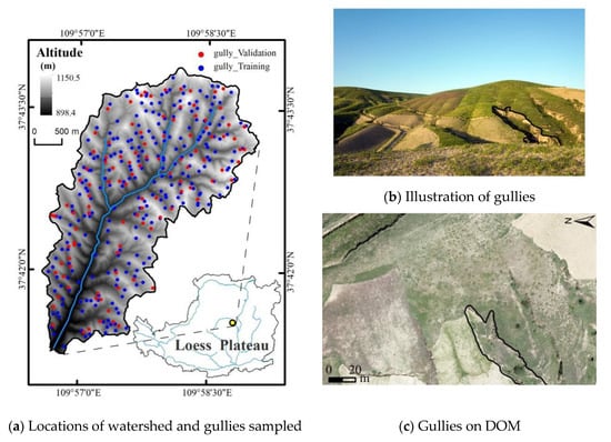
Figure 1.
Study area.
2.2. Base Data and Data Processing
The base datasets included digital orthophoto maps (DOM) and digital surface models (DSM) and were obtained using Unmanned Arial Vehicles (UAV). The drone used was a DJI 4 RTK, and the ground image control points were set up to improve the data accuracy. The Pix4dmapper software was used for data processing; it is based on image content, uses unique optimization techniques and regional network adjustment techniques to calibrate images, and can generate the DSM and DOM automatically and quickly. The resolution of DOM and DSM was 0.09 m. The DSM was resampled to 1 m for later use. The DOM and DSM datasets were obtained on 28 August 2019. Gaussian filtering was applied to reduce the effects of noise.
Vegetation is an important source of ground elevation error when using UAV-sourced datasets. In this study area, most of the hillslopes were covered by a low and relatively homogeneous height of grass or were bare land during the time of the flight. We assumed this had limited influence on the later analyses. There are some trees at the bottom of the valleys and on a tiny part of the hillslope. In these areas, the points with surface elevation values around the trees were obtained manually. Then, the 1 m-resolution DSM in these places was obtained by interpolation based on those points and mosaiced to the resampled 1 m DSM to make the final DSM dataset.
We used RTK GNSS instruments composed of base stations and mobile stations to carry out field measurements. The mobile station simultaneously receives the observation data from the base station broadcast, and the mobile station antenna receives the observation data from the satellite, which forms the RTK observation model [33]. Its horizontal precision is 2.5 mm ± 2 ppm and its vertical precision is 5 mm ± 2 ppm.
2.3. Experimental Procedure
The basic procedure of the experiment included five steps (Figure 2). In Step 1, the base datasets including DOM, DSM, gully erosion inventory map, and gully erosion conditioning factors were obtained. Step 2 was multi-collinearity analysis using tolerance and variance inflation factor (VIF); in Step 3, the relative importance of conditioning factor classes to gully erosion locations was determined using the weight of evidence model; Step 4 was gully erosion susceptibility mapping using RF, GBDT, and XGBoost; and Step 5 was validation through AUC. About 30 % (in number) of gullies belonged to testing datasets, which were used for validation. The other 70% of gullies belonged to the training dataset, which was used for model building.
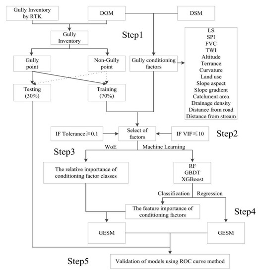
Figure 2.
Study flow diagram.
2.4. Gully Erosion Inventory Mapping
Gully erosion inventory mapping is essential for GESM since it is the base dataset for model building and validation [34]. The gully erosion inventory map used in this research was obtained by visual interpretation based on 0.09 m DOM.
Stratified random sampling was used for selecting the interpreted gullies used for gully erosion inventory mapping. The study area was firstly divided into 30 sub-watersheds based on hydrological analysis; then, the numbers and locations of the selected gullies were determined according to the watershed area and geomorphological types in each sub-watershed. The drainage area for each selected gully was chosen as the corresponding non-gully sample. There were other types of non-gully areas, such as construction land, cultivated land, water body, and so on. We selected these non-gully areas with a square with a side length of 10 m as a unit. In total, 353 gully polygons were selected, 70% (247 gullies) were used in the model building, and the remaining 30% (106 gullies) were used for the model validation; 502 non-gully polygons were selected, 70% (351 non-gullies) were used in the building of the model, and the remaining 30% (151 non-gullies) were used for the validation. The selected gullies range in length from more than ten meters to hundreds of meters and width from a few meters to dozens of meters. Many gullies hang on both sides of the gully, and the elevation continues to drop from the head of the gully. The shape of the gullies is mostly V-shaped.
The accuracy of the visually interpreted gullies was validated based on 32 field-measured gully data obtained using GNSS RTK (Figure 3) using Equations (1) to (4) [29,30]. The accuracy was 96.78%, which showed the interpreted results were of sufficient accuracy for use.
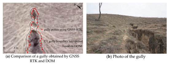
Figure 3.
Comparison of a gully obtained by GNSS RTK and DOM, and photo of a gully in the study area.
In these equations, M is the field measured area of the gully, V indicates the gully area obtained by visual interpretation of DOM, I is the intersection area of A and B, N is the number of gullies, and Precision is the overall accuracy.
2.5. Gully Erosion Conditioning Factors
An important task is to select practical geo-environmental factors to assess gully erosion susceptibility, as they influence the prediction quality of the models [14]. There is no global consensus or universal regulation for the selection of gully conditioning factors. Based on previous studies [6,20,35], available data, and field perceptions of the study area, we selected a total of 14 conditioning factors (Figure 4) for GESM. These factors are the slope gradient, slope aspect, altitude, curvature, topographic wetness index (TWI), stream power index (SPI), drainage density, distance from the stream, land use, distance from the road, catchment area, distribution of terrace, slope length (LS), and fractional vegetation cover (FVC). In this study, we used ArcGIS 10.5 to extract topographic factors such as slope aspect, slope gradient, curvature, TWI, SPI, LS, and catchment area from the digital elevation model and the DOM was used to extract land use, stream network, and road distribution maps, FVC, and terraced fields. Subsequently, the layers of distance from stream and road, as well as drainage density, were produced using the Euclidean distance and Line density tools in ArcGIS 10.5 software, respectively.
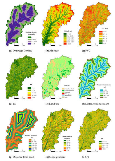
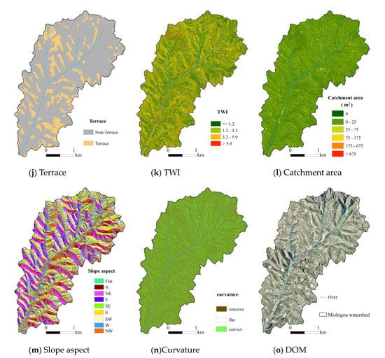
Figure 4.
Gully erosion conditioning factors: (a) Drainage Density, (b) Altitude, (c) FVC, (d) LS, (e) Land use, (f) Distance from stream, (g) Distance from road, (h) Slope gradient, (i) SPI, (j) Terrace, (k) TWI, (l) Catchment area, (m) Slope aspect, and (n) Curvature (o) DOM.
2.6. Multi-Collinearity Assessment
One of the most critical steps in GESM is to analyze the correlation or the influence of multi-collinearity among different influence factors. Multi-collinearity is a condition under which independent variables are highly correlated or interrelated [36]. Tolerance and variance inflation factor (VIF) are two essential indexes used to identify the relationship between independent variables [37]. A tolerance value less than 0.1 or a VIF value larger than 10 indicates a high multi-collinearity [38], in which case it is necessary to remove those specific variables. Otherwise, the accuracy of the prediction will decline [39].
2.7. Gully Erosion Modeling
2.7.1. Weight of Evidence Model (WoE)
WoE is a bivariate statistical method based on the Bayesian probability framework to estimate the relative importance of conditioning factor classes [40]. In this study, the model was used to determine the weight values of conditioning factor classes to gully erosion locations; the weights were calculated using Equations (5) to (11).
where P is the probability and ln is the natural log function. B is the presence of gully conditioning factor and is the absence of gully conditioning factor. L is the presence of gully and is the absence of gully. and indicate that the conditioning factor is present (positive correlation) and absent (negative correlation), respectively. C indicates the overall association between gully occurrence and conditioning factors. S(C) is the standard deviation of the contrast. is the variance of the and is the variance of , and W is the weight value of each factor for a specific class.
Each continuous conditioning factor was reclassified into a finite set of subclasses to calculate the proportion of gully and non-gully data in each class. We used the natural break method to classify the influence factors in order to highlight the differences at all levels, and the number of grades refers to the previous literature [20,21,30].
2.7.2. Machine Learning Models
- (1)
- Random forest (RF);
Breiman [41] defines a random forest as a collection of tree-structured weak learners comprised of identically distributed random vectors where each tree contributes to a prediction for x. The random forest ML model is a nonparametric multivariate model consisting of multiple trees and can be used for classification and regression [6]. In each splitting process of the subtree in the random forest, a certain number of the data and features are randomly selected, and then the optimal value is obtained. In this way, the decision trees in the random forest can be different from each other, enhance the diversity of the system, and thus improve the performance of the model [42]. For the classification problem, the result of the simple majority voting method is used as the output of the random forest; for the regression problem, the simple average of the output result of a single tree is taken as the output of the random forest. The construction of the RF model was realized by using the scikit-learn library in Python.
- (2)
- Gradient boosted fecision trees (GBDT);
GBDT is an ensemble machine learning method combining multiple decision trees based on the boosting concept. It continuously improves prediction accuracy through interactions. A new decision tree was established in the gradient direction of the reducing residuals in each iteration [43]. The GBDT tree is constructed sequentially. That is, the first tree trains all the samples to get a model and its weight, while the latter tree continues to train the sample to get a model and weight with the goal of reducing the residual of the previous tree, and stop when the residual is small enough or reach the set number of trees. The final model is the weighted sum results of each tree. GBDT can be used for classification and regression problems, and it is regarded as one of the best algorithms for fitting actual distributions [44].
- (3)
- Extreme gradient boosting machine (XGBoost);
The XGBoost was introduced by Chen and Guestrin [45] based on the concept of boosting. XGBoost produces a prediction model in the form of a boosting ensemble of weak classification trees by a gradient descent that optimizes the loss function [46,47]. This algorithm first builds all the subtrees that can be built from top to bottom, then prunes backward from bottom to top so that local optimal solutions can be avoided [48]. It is more efficient and can be used for both classification and regression tasks. XGBoost has three crucial aspects. These are a regularized objective function for better generalization, gradient tree boosting for additive training, and shrinkage and column subsampling to preventing overfitting [45,49].
The optimal parameter combination can be explored by a learning curve or grid search algorithm, and the ranking of feature importance can be obtained by using the Feature_importance interface based on Gini index calculation; Gini index is a common parameter to evaluate the importance of factors in GESM [6,18,30]. Feature importance refers to the contribution rate of variables to fitting accuracy. A specific factor is more important if its feature importance is larger. The reasons for selecting these models are the following: (1) XGBoost is an efficient algorithm that has the capacity to find missing values and enhance the prediction performance result. It represents the state-of-the-art within the machine learning community. At present, it has seldom been used in gully erosion susceptibility mapping. (2) The XGBoost algorithm is improved on the basis of the GBDT algorithm, and the selection of GBDT algorithm can more effectively utilize the improvement effect of XGBoost. (3) The RF model is one of the most widely used models in gully erosion susceptibility mapping, and has achieved excellent simulation results. (4) Each of the three models is an ensemble model, which can remove the shortcomings of individual statistical or ML models [18].
2.8. Model Validation
We used 30% of the gullies which were not included in the modeling process to validate the GESM based on the receiver operating characteristic (ROC) curve and calculation of the area under the curve (AUC). A ROC curve effectively indicates the quality of deterministic and probabilistic models and forecast systems [50,51]. The x-axis and y-axis of the ROC curve are plotted for 1-specificity and sensitivity, respectively, and have different cut-off thresholds. X represents the sensitivity of the true positive rate (TPR), the value of the predicted gully pixel. The real case is the gully pixel, which accounts for the ratio of the gully pixel value in all real cases. Y represents the false positive rate (FPR), that is, the value that is predicted as gully pixels, but the real situation is non-gully pixels, which accounts for the ratio of non-gully pixels in all real cases. The AUC value is a quantitative value to evaluate the ROC curve. When the AUC value is 0.5, the prediction effect of the model is no better than the random method to predict the occurrence of gullies. When ideally, that is, a complete distinction between gully and non-gully pixels, the value of AUC is 1., and the closer the ROC curve is to the upper left corner, the more accurate it is [35]. The AUC value and prediction accuracy can be classified as follows: 0.5–0.6, poor; 0.6–0.7, average; 0.7–0.8, good; 0.8–0.9, very good; and 0.9–1, excellent [30]. The ROC-AUC can be calculated by Equations (12) to (14).
where TP is true positive, TN is true negative, FP is false positive and FN is false negative. P and N represent the presence and absence of gullies, respectively.
3. Results
3.1. Results of the Collinearity among Factors
Table 1 presents the multi-collinearity values for the 14 factors which are commonly used in gully erosion susceptibility mapping. Most of the factors in Table 1 met the requirements of multi-collinearity analysis (VIF ≤ 10, Tolerance ≥ 0.1), except for the factor of the existence of terrace, and could be used in the following analysis.

Table 1.
Multi-collinearity test among gully erosion conditioning factors.
3.2. Importance of Conditioning Factors to Gully Erosion
Both the relative importance of conditioning factor classes and the feature importance of conditioning factors to gully erosion were evaluated.
The relative importance of conditioning factor classes to gully erosion locations using the WoE method is presented in Table 2. The weight values were higher in one or a few classes than that of the other classes for each factor. With altitude, slope gradient, and FVC increase, the weight values increased and then decreased, which showed that areas with medium values of the above factors were easier for gully formation. The weight values were the highest for the altitude values from 1000 m to 1035 m, slope gradient values from 40°to 50° and FVC values from 41% to 58%. The weight values increased with LS factor and catchment area drainage density, and SPI values also became larger. The weight values were largest when TWI, curvature, and distance from the stream were small. In addition, the weight value was the highest when the slope aspect was N–facing slopes, and the distance from the road was 385–485 m. Gully erosion is more likely to occur in this area if the values of altitude, slope gradient, FVC, and the distance from the road are medium, LS factor, catchment area, drainage density, and SPI values are larger, and TWI, distance from the stream, and curvature are smallest. N–facing slope tends to have more gullies formation than the other slope aspects. The weight values in Table 2 were calculated based on Pixels of Gullies, Pixels of Non-gullies, and Equations (5) to (11).
Table 2.
The relative importance of conditioning factor classes to gully erosion locations using the weights-of-evidence (WoE) model.
Figure 5 shows the feature importance of conditioning factors based on the MLC models. It showed that, compared with other factors, slope gradient, land use, and altitude were the most critical factors in predicting GESM for each of the three selected machine learning algorithms, the RF model, GBDT model, and the XGBoost model. The distribution of gullies in this area is mainly affected by terrain and man-made factors.
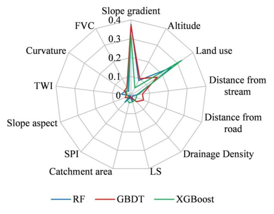
Figure 5.
The importance of factors in different models.
3.3. Gully Erosion Susceptibility Mapping (GESM)
GESM using each of the selected models is shown in Figure 6. The natural break method was used to divide the map into five different grades; these were “very low”, “low”, “medium”, “high”, and “very high”. Generally, the GESM results were consistent using the combined WoE-MLC and machine learning models by themselves. Higher susceptibility zones are mainly located in the middle of the hillslopes at both sides of streams banks. Lower or medium susceptibility zones are mainly located on the top of hillslopes and the bottom of the streams. The maps obtained from WoE-MLC models were more fragmented than those from the machine learning models. More very low susceptibility areas were predicted on top of the hillslopes by using machine learning models.
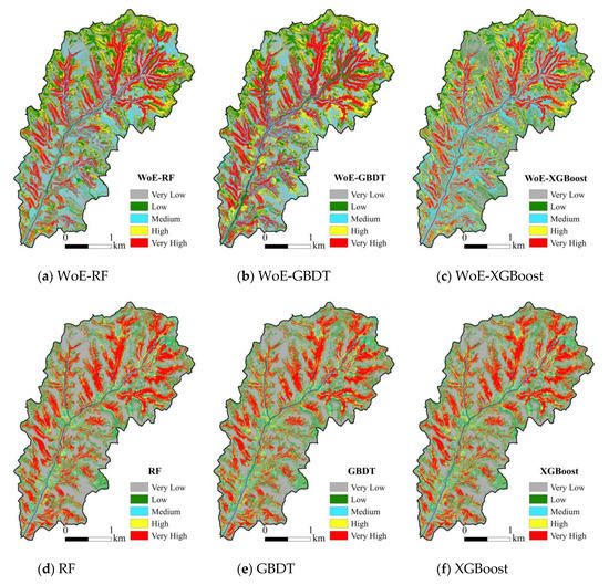
Figure 6.
Gully erosion susceptibility maps by different models: (a) WoE-RF, (b) WoE-GBDT, (c) WoE-XGBoost, (d) RF, (e) GBDT, and (f) XGBoost.
3.4. Validation of Models
The GESM prediction accuracy of the six models is shown in Figure 7. The results showed that the AUC values of the six models were between 0.925 and 0.957, indicating high prediction accuracy for all models. The average AUC value of the three WoE-MLC models was 0.931, still acceptable, although slightly lower than that of the machine learning models (0.954). The AUC values for the XGBoost algorithm, combined with WoE or as a separate machine learning regression method, were higher than that of RF and GBDT algorithms without WOE.
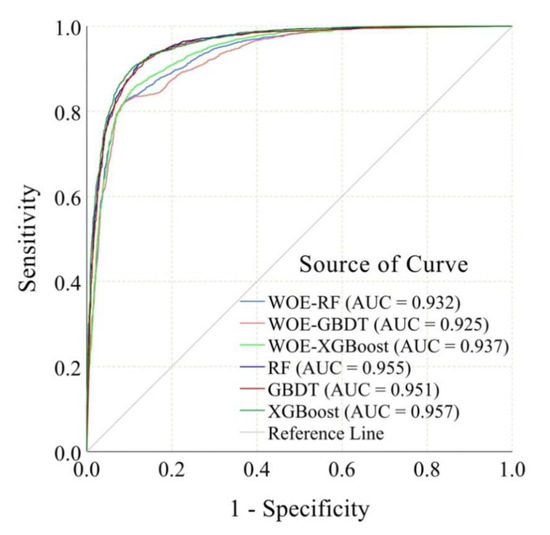
Figure 7.
The receiver operating characteristic (ROC) curve using testing data.
4. Discussion
We hypothesized that combining the WoE model and MLC model was a useful method for GESM, being more efficient and easier to interpret the influence of the varied factors for gully formation, and terrain-related factors should be the most critical factor for GESM in complex terrain areas. By exploring three commonly used ML regression models and WoE-MLC models, the findings of this study supported our hypothesis.
4.1. Rationale for Gully Erosion Susceptibility Mapping
The high gully susceptibility zones predicted by all of the models used in this research were mainly located in the middle of the hillslopes on both sides of stream banks, which is consistent with the prediction of Ding et al. [52]. Low or medium susceptibility zones are mainly located on the top of hillslopes and at the bottom of the streams (Figure 6). This spatial distribution was reasonable according to field investigation and UAV-sourced DOM (Figure 1b). There are more gullies in the middle of the hillslopes in the Loess Plateau because the slope gradient usually is larger than 30°, larger than the other parts of the hillslope, and the catchment area is large enough for gully formation. On the top of hillslopes, the slope gradient is smaller than downwards of the hillslopes, and the drainage area is usually smaller, which makes the gully erosion susceptibility lower. At the bottom of the valleys in the Loess Plateau, although the catchment area usually is large, there are generally few gullies found since the terrain is relatively flat. Its main function is to transport the sediment generated by gully erosion to other places [37].
The gully classification in the Loess Plateau area is more complicated than in other areas because of its complex terrain surface [53,54]. Different susceptibility maps of gully erosion are often obtained based on different gully types. For example, the gully maps predicted by Dai et al. [55] and Yang et al. [56] were different from those in this research. Their method was to determine the gully area by illuminating the surface of the gully, simulating the shadows on the shaded slopes, and then merging both sides of the shadows, so the gully map obtained included the bottom of the streams. Based on a 12.5 m DEM and other conditioning factors, Lei et al. [57] and Azedou et al. [58] predicted gully erosion susceptibility maps in the Robat Turk watershed and the rural municipality of El Faid, respectively. The gullies with smaller shapes were difficult to express at that coarser resolution, so the gully areas simulated tended to be more concentrated. This research mainly focused on the gullies caused by modern accelerated water erosion, which are much smaller and mainly distributed in the middle of the hillslopes. This type of gully was more active and was at the most serious stage of water erosion, so the damage to land resources was greater.
The spatial resolution of all the factors we used was 1 m, at which scale it might be challenging to avoid the influence of the micro-topography on the analysis [59]. Some studies have shown that the best resolution did not necessarily provide the best information [35]. Therefore, it is necessary to analyze the accuracy of gully erosion susceptibility maps at different spatial resolutions to decide the best or least the necessary spatial resolution.
4.2. Variable Importance and GESM Model Comparison
Although many researchers have used different factors in predicting gully erosion susceptibility, there are no universal rules with which to select independent variables for GESM modeling. In this research, we explored the contribution of independent variables to gully erosion susceptibility mapping in complex areas of the Loess Plateau. The result showed that slope gradient, land use, and altitude were the most important factors based on all the three machine learning models used. Gayen et al. [20] found in the Pathro River Basin of India, land use and altitude were the most critical factors affecting the occurrence of local gullies, while the importance of slope gradient was low. The terrain of the study area is much flatter in their study (less than 8.6° in 89% of the study area) than in this research (with an averaged slope gradient value of 28.7°, larger than 30° in 48% of the study area). Slope gradient seems to be more important for GESM when the terrain is more complex. Studies by Pourghasemi et al. [34] in the southeast part of Golestan Province suggested that the distance from the stream, drainage density, and altitude were the more important conditioning factors. The study of Arabameri et al. [60] in the Najafabad watershed showed that drainage density, altitude, and LU were more important factors. It can be seen that the most critical factors affecting gully susceptibility may be different according to different study areas. The factor importance for different geomorphological types needs to be further studied.
According to the results of this research, the AUC values of the machine learning models were slightly higher than those of the WoE-MLC models. Machine learning models are based on each conditioning factor and use the pixel-by-pixel model to produce the GESM. WoE-MLC models utilize the feature importance of conditioning factors obtained from the machine learning classification model and the relative importance of conditioning factor classes obtained from the WoE model and then use raster calculation to create GESM. The pixel-by-pixel approach adopted by machine learning models would theoretically obtain more precise results than WoE-MLC models but is much more time-consuming and harder for interpretation. Although the accuracy of the WoE-MLC models is relatively lower (averaged AUC = 0.931), it is still acceptable since WoE-MLC models are more computationally efficient and interpretable than machine learning models. WoE-MLC models are of great potential for gully susceptibility mapping in large regions or at high resolution and in other situations where a large amount of data is needed. Many studies have used statistical and machine learning models to evaluate the relationship between gully occurrence and conditioning factors in different regions, and we believe that the method will be widely applicable.
The XGBoost algorithm was higher in prediction accuracy than the RF and GBDT algorithms. In order to know which algorithm was stronger in generalization ability, we used the training set to verify the GESM predicted by the three algorithms. It showed that the AUC values of XGBoost, RF, and GBDT were 0.958, 0.989, and 0.992, respectively. Although RF and GBDT performed well in the training set, their performance in the testing set was relatively poor according to the result in Figure 7, indicating that they were more influenced by overfitting. The XGBoost algorithm has a stronger generalization ability and can avoid overfitting more effectively. Additionally, the research of Ding et al. [52] showed that the XGBoost algorithm is more time-efficient, and this advantage gradually expands with the increase of the number of conditioning factors. At present, many studies have concluded that the RF algorithm has achieved better simulation results in gully erosion susceptibility mapping [20,37,61,62]. The XGBoost algorithm has been widely used in landslide susceptibility mapping [49], flash-flood susceptibility mapping [63], and groundwater vulnerability predictive mapping [64], and excellent simulation results have been achieved. However, there has been less application in gully erosion susceptibility mapping, and further research is still needed to fully evaluate the application of the XGBoost algorithm in gully mapping.
4.3. Future Work and Applications
In recent years, the deep neural learning network (DLNN), which is composed of fully convolutional neural networks (CNNs), deep belief networks (DBNs), stacked auto-encoder (SAE) networks, etc. [65], has become very popular [66]. Band et al. [67] suggested that the DLNN model can scientifically build a high-level feature from a raw dataset. It consists of a different topology than the general neural network of a single hidden layer, as more than one hidden layer is present in this algorithm. Their research found that the DLNN algorithm was more powerful for gully erosion susceptibility mapping than the traditional ML algorithm. However, the DLNN algorithm will have similar time-consuming problems as other ML algorithms, and more effort is needed in the future to solve this problem to meet the needs of gully mapping at a large scale.
With the development of fine-resolution images all over the world [59], large-scale modeling of gully maps will be possible and would be an urgent need for research and management. The results of this research offered a time-efficient, interpretable, and relatively accurate method for gully mapping and would be well applied in future large-scale gully modeling.
5. Conclusions
This study explored the gully erosion susceptibility mapping method in a watershed with highly complex terrain in the Loess Plateau of China. Three commonly used machine learning models were used, among which the prediction accuracy of XGBoost is higher than that of RF and GBDT. According to the feature importance of influence factors, slope gradient, land use, and altitude were the most important factors for gully mapping. Combing the weight of evidence and the machine learning classification model is a computationally efficient and interpretable way to implement gully susceptibility mapping.
Author Contributions
Conceptualization, Annan Yang and Chunmei Wang; methodology, Annan Yang, Chunmei Wang and Yongqing Long; software, Annan Yang and Yongqing Long; validation, Yongqing Long; investigation, Guowei Pang; resources, Guowei Pang, Yongqing Long and Lei Wang; data curation, Yongqing Long and Lei Wang; writing—original draft preparation, Annan Yang; writing—review and editing, Chunmei Wang Yongqing Long, Richard M. Cruse and Qinke Yang; project administration, Chunmei Wang; research group leader, Qinke Yang All authors have read and agreed to the published version of the manuscript.
Funding
This research was funded by the National Natural Science Foundation of China, Grant No. 41977062, 41601290, and 41930102, SKL Foundation Grant No. A314021402-2016, the Strategic Priority Research Program of the Chinese Academy of Sciences, Grant No. XDA20040202, Program for Key Science and Technology Innovation Team in Shaanxi Province, Grant No. 2014KCT-27.
Data Availability Statement
Please refer to suggested Data Availability Statements in section “MDPI Research Data Policies” at https://www.mdpi.com/ethics.
Conflicts of Interest
The authors declare no conflict of interest.
References
- Poesen, J.; Nachtergaele, J.; Verstraeten, G.; Valentin, C. Gully erosion and environmental change: Importance and research needs. CATENA 2003, 50, 91–133. [Google Scholar] [CrossRef]
- Castillo, C.; Gómez, J.A. A century of gully erosion research: Urgency, complexity and study approaches. Earth-Sci. Rev. 2016, 160, 300–319. [Google Scholar] [CrossRef]
- Dotterweich, M.; Rodzik, J.; Zgłobicki, W.; Schmitt, A.; Schmidtchen, G.; Bork, H.-R. High resolution gully erosion and sedimentation processes, and land use changes since the Bronze Age and future trajectories in the Kazimierz Dolny area (Nałęczów Plateau, SE-Poland). CATENA 2012, 95, 50–62. [Google Scholar] [CrossRef]
- Chaplot, V. Impact of terrain attributes, parent material and soil types on gully erosion. Geomorphology 2013, 186, 1–11. [Google Scholar] [CrossRef]
- Kirkby, M.; Bracken, L. Gully processes and gully dynamics. Earth Surf. Process. Landf. 2009, 34, 1841–1851. [Google Scholar] [CrossRef]
- Rahmati, O.; Tahmasebipour, N.; Haghizadeh, A.; Pourghasemi, H.R.; Feizizadeh, B. Evaluation of different machine learning models for predicting and mapping the susceptibility of gully erosion. Geomorphology 2017, 298, 118–137. [Google Scholar] [CrossRef]
- Torri, D.; Poesen, J. A review of topographic threshold conditions for gully head development in different environments. Earth-Sci. Rev. 2014, 130, 73–85. [Google Scholar] [CrossRef]
- Chaplot, V.; Coadou le Brozec, E.; Silvera, N.; Valentin, C. Spatial and temporal assessment of linear erosion in catchments under sloping lands of northern Laos. CATENA 2005, 63, 167–184. [Google Scholar] [CrossRef]
- Majhi, A.; Nyssen, J.; Verdoodt, A. What is the best technique to estimate topographic thresholds of gully erosion? Insights from a case study on the permanent gullies of Rarh plain, India. Geomorphology 2021, 375, 107547. [Google Scholar] [CrossRef]
- Dewitte, O.; Daoudi, M.; Bosco, C.; Van Den Eeckhaut, M. Predicting the susceptibility to gully initiation in data-poor regions. Geomorphology 2015, 228, 101–115. [Google Scholar] [CrossRef]
- Vanmaercke, M.; Panagos, P.; Vanwalleghem, T.; Hayas, A.; Foerster, S.; Borrelli, P.; Rossi, M.; Torri, D.; Casalí, J.; Borselli, L.; et al. Measuring, modelling and managing gully erosion at large scales: A state of the art. Earth-Sci. Rev. 2021, 218, 103637. [Google Scholar] [CrossRef]
- Conoscenti, C.; Angileri, S.; Cappadonia, C.; Rotigliano, E.; Agnesi, V.; Märker, M. Gully erosion susceptibility assessment by means of GIS-based logistic regression: A case of Sicily (Italy). Geomorphology 2014, 204, 399–411. [Google Scholar] [CrossRef] [Green Version]
- Arabameri, A.; Rezaei, K.; Pourghasemi, H.R.; Lee, S.; Yamani, M. GIS-based gully erosion susceptibility mapping: A comparison among three data-driven models and AHP knowledge-based technique. Environ. Earth Sci. 2018, 77, 628. [Google Scholar] [CrossRef]
- Conoscenti, C.; Di Maggio, C.; Rotigliano, E. Soil erosion susceptibility assessment and validation using a geostatistical multivariate approach: A test in Southern Sicily. Nat. Hazards 2008, 46, 287–305. [Google Scholar] [CrossRef]
- Arabameri, A.; Pradhan, B.; Rezaei, K.; Yamani, M.; Pourghasemi, H.R.; Lombardo, L. Spatial modelling of gully erosion using evidential belief function, logistic regression, and a new ensemble of evidential belief function-logistic regression algorithm. Land Degrad. Dev. 2018, 29, 4035–4049. [Google Scholar] [CrossRef]
- Conforti, M.; Aucelli, P.P.C.; Robustelli, G.; Scarciglia, F. Geomorphology and GIS analysis for mapping gully erosion susceptibility in the Turbolo stream catchment (Northern Calabria, Italy). Nat. Hazards 2011, 56, 881–898. [Google Scholar] [CrossRef]
- Arabameri, A.; Cerda, A.; Tiefenbacher, J.P. Spatial pattern analysis and prediction of gully erosion using novel hybrid model of entropy-weight of evidence. Water 2019, 11, 1129. [Google Scholar] [CrossRef] [Green Version]
- Chowdhuri, I.; Pal, S.C.; Arabameri, A.; Saha, A.; Chakrabortty, R.; Blaschke, T.; Pradhan, B.; Band, S.S. Implementation of artificial intelligence based ensemble models for gully erosion susceptibility assessment. Remote. Sens. 2020, 12, 3620. [Google Scholar] [CrossRef]
- Arabameri, A.; Chandra Pal, S.; Costache, R.; Saha, A.; Rezaie, F.; Seyed Danesh, A.; Pradhan, B.; Lee, S.; Hoang, N.-D. Prediction of gully erosion susceptibility mapping using novel ensemble machine learning algorithms. Geomat. Nat. Hazards Risk 2021, 12, 469–498. [Google Scholar] [CrossRef]
- Gayen, A.; Pourghasemi, H.R.; Saha, S.; Keesstra, S.; Bai, S. Gully erosion susceptibility assessment and management of hazard-prone areas in India using different machine learning algorithms. Sci. Total Environ. 2019, 668, 124–138. [Google Scholar] [CrossRef]
- Arabameri, A.; Chen, W.; Loche, M.; Zhao, X.; Li, Y.; Lombardo, L.; Cerda, A.; Pradhan, B.; Bui, D.T. Comparison of machine learning models for gully erosion susceptibility mapping. Geosci. Front. 2020, 11, 1609–1620. [Google Scholar] [CrossRef]
- Saha, S.; Roy, J.; Arabameri, A.; Blaschke, T.; Tien Bui, D. Machine learning-based gully erosion susceptibility mapping: A case study of Eastern India. Sensors 2020, 20, 1313. [Google Scholar] [CrossRef] [PubMed] [Green Version]
- Wang, C.; Cruse, R.M.; Gelder, B.; James, D.; Liu, X. Grid order prediction of ephemeral gully head cut position: Regional scale application. CATENA 2021, 200, 105158. [Google Scholar] [CrossRef]
- Polykretis, C.; Ferentinou, M.; Chalkias, C. A comparative study of landslide susceptibility mapping using landslide susceptibility index and artificial neural networks in the Krios River and Krathis River catchments (northern Peloponnesus, Greece). Bull. Eng. Geol. Environ. 2015, 74, 27–45. [Google Scholar] [CrossRef]
- Tehrany, M.S.; Pradhan, B.; Jebur, M.N. Spatial prediction of flood susceptible areas using rule based decision tree (DT) and a novel ensemble bivariate and multivariate statistical models in GIS. J. Hydrol. 2013, 504, 69–79. [Google Scholar] [CrossRef]
- Arabameri, A.; Cerda, A.; Pradhan, B.; Tiefenbacher, J.P.; Lombardo, L.; Bui, D.T. A methodological comparison of head-cut based gully erosion susceptibility models: Combined use of statistical and artificial intelligence. Geomorphology 2020, 359, 107136. [Google Scholar] [CrossRef]
- Meliho, M.; Khattabi, A.; Mhammdi, N. A GIS-based approach for gully erosion susceptibility modelling using bivariate statistics methods in the Ourika watershed, Morocco. Environ. Earth Sci. 2018, 77, 1–14. [Google Scholar] [CrossRef]
- Rahmati, O.; Haghizadeh, A.; Pourghasemi, H.R.; Noormohamadi, F. Gully erosion susceptibility mapping: The role of GIS-based bivariate statistical models and their comparison. Nat. Hazards 2016, 82, 1231–1258. [Google Scholar] [CrossRef]
- Nampak, H.; Pradhan, B.; Mojaddadi Rizeei, H.; Park, H.-J. Assessment of land cover and land use change impact on soil loss in a tropical catchment by using multitemporal SPOT-5 satellite images and Revised Universal Soil Loss Equation model. Land Degrad. Dev. 2018, 29, 3440–3455. [Google Scholar] [CrossRef]
- Arabameri, A.; Pradhan, B.; Pourghasemi, H.R.; Rezaei, K.; Kerle, N. Spatial modelling of gully erosion using GIS and R programing: A comparison among three data mining algorithms. Appl. Sci. 2018, 8, 1369. [Google Scholar] [CrossRef] [Green Version]
- Shit, P.K.; Bhunia, G.S.; Pourghasemi, H.R. Gully Erosion Susceptibility Mapping Based on Bayesian Weight of Evidence. In Gully Erosion Studies from India and Surrounding Regions; Shit, P.K., Pourghasemi, H.R., Bhunia, G.S., Eds.; Springer International Publishing: Cham, Switzerland, 2020; pp. 133–146. [Google Scholar]
- Zhu, T.X. Gully and tunnel erosion in the hilly Loess Plateau region, China. Geomorphology 2012, 153, 144–155. [Google Scholar] [CrossRef]
- Petovello, M.G.; Curran, J.T. Simulators and Test Equipment; Springer International Publishing: New York, NY, USA, 2017; pp. 535–558. [Google Scholar]
- Pourghasemi, H.R.; Sadhasivam, N.; Kariminejad, N.; Collins, A.L. Gully erosion spatial modelling: Role of machine learning algorithms in selection of the best controlling factors and modelling process. Geosci. Front. 2020, 11, 2207–2219. [Google Scholar] [CrossRef]
- Garosi, Y.; Sheklabadi, M.; Pourghasemi, H.R.; Besalatpour, A.A.; Conoscenti, C.; Van Oost, K. Comparison of differences in resolution and sources of controlling factors for gully erosion susceptibility mapping. Geoderma 2018, 330, 65–78. [Google Scholar] [CrossRef]
- Alin, A. Multicollinearity. Wiley Interdiscip. Rev. Comput. Stat. 2010, 2, 370–374. [Google Scholar] [CrossRef]
- Amiri, M.; Pourghasemi, H.R.; Ghanbarian, G.A.; Afzali, S.F. Assessment of the importance of gully erosion effective factors using Boruta algorithm and its spatial modeling and mapping using three machine learning algorithms. Geoderma 2019, 340, 55–69. [Google Scholar] [CrossRef]
- Pourghasemi, H.R.; Beheshtirad, M.; Pradhan, B. A comparative assessment of prediction capabilities of modified analytical hierarchy process (M-AHP) and Mamdani fuzzy logic models using Netcad-GIS for forest fire susceptibility mapping. Geomat. Nat. Hazards Risk 2016, 7, 861–885. [Google Scholar] [CrossRef] [Green Version]
- Kuhnert, P.; Kinsey-Henderson, A.; Bartley, R.; Herr, A. Incorporating uncertainty in gully erosion calculations using the random forest modelling approach. Environmetrics 2009, 21, 493–509. [Google Scholar] [CrossRef]
- Xie, Z.; Chen, G.; Meng, X.; Zhang, Y.; Qiao, L.; Tan, L. A comparative study of landslide susceptibility mapping using weight of evidence, logistic regression and support vector machine and evaluated by SBAS-InSAR monitoring: Zhouqu to Wudu segment in Bailong River Basin, China. Environ. Earth Sci. 2017, 76, 313. [Google Scholar] [CrossRef]
- Breiman, L. Random forests. Mach. Learn. 2001, 45, 5–32. [Google Scholar] [CrossRef] [Green Version]
- Liaw, A.; Wiener, M. Classification and regression by randomForest. R. News 2002, 2, 18–22. [Google Scholar]
- He, Q.; Jiang, Z.; Wang, M.; Liu, K. Landslide and wildfire susceptibility assessment in southeast asia using ensemble machine learning methods. Remote. Sens. 2021, 13, 1572. [Google Scholar] [CrossRef]
- Song, Y.; Niu, R.; Shiluo, X.; Ye, R.; Peng, L.; Guo, T.; Li, S.; Chen, T. Landslide susceptibility mapping based on weighted gradient boosting decision tree in Wanzhou section of the Three Gorges Reservoir Area (China). ISPRS Int. J. Geo-Inf. 2018, 8, 4. [Google Scholar] [CrossRef] [Green Version]
- Chen, T.; Guestrin, C. XGBoost: A Scalable Tree Boosting System. In Proceedings of the 22nd Acm Sigkdd International Conference on Knowledge Discovery and Data Mining, San Francisco, CA, USA, 13–17August 2016; pp. 785–794. [Google Scholar]
- Cui, Y.; Cai, M.; Stanley, H.E. Comparative Analysis and Classification of Cassette Exons and Constitutive Exons. BioMed Res. Int. 2017, 2017, 7323508. [Google Scholar] [CrossRef] [PubMed] [Green Version]
- Sahin, E.K. Assessing the predictive capability of ensemble tree methods for landslide susceptibility mapping using XGBoost, gradient boosting machine, and random forest. SN Appl. Sci. 2020, 2, 1308. [Google Scholar] [CrossRef]
- Dev, V.A.; Eden, M.R. Formation lithology classification using scalable gradient boosted decision trees. Comput. Chem. Eng. 2019, 128, 392–404. [Google Scholar] [CrossRef]
- Can, R.; Kocaman, S.; Gokceoglu, C. A Comprehensive assessment of XGBoost algorithm for landslide susceptibility mapping in the upper basin of Ataturk Dam, Turkey. Appl. Sci. 2021, 11, 4993. [Google Scholar] [CrossRef]
- Azareh, A.; Rahmati, O.; Rafiei-Sardooi, E.; Sankey, J.B.; Lee, S.; Shahabi, H.; Ahmad, B.B. Modelling gully-erosion susceptibility in a semi-arid region, Iran: Investigation of applicability of certainty factor and maximum entropy models. Sci. Total Environ. 2019, 655, 684–696. [Google Scholar] [CrossRef]
- Yesilnacar, E.; Topal, T. Landslide susceptibility mapping: A comparison of logistic regression and neural networks methods in a medium scale study, Hendek region (Turkey). Eng. Geol. 2005, 79, 251–266. [Google Scholar] [CrossRef]
- Ding, H.; Liu, K.; Chen, X.; Xiong, L.; Tang, G.; Qiu, F.; Strobl, J. Optimized segmentation based on the weighted aggregation method for loess bank gully mapping. Remote Sens. 2020, 12, 793. [Google Scholar] [CrossRef] [Green Version]
- Jin, F.; Yang, W.; Fu, J.; Li, Z. Effects of vegetation and climate on the changes of soil erosion in the Loess Plateau of China. Sci. Total Environ. 2021, 773, 145514. [Google Scholar] [CrossRef]
- Wu, Y.; Cheng, H. Monitoring of gully erosion on the Loess Plateau of China using a global positioning system. CATENA 2005, 63, 154–166. [Google Scholar] [CrossRef]
- Dai, W.; Yang, X.; Na, J.; Li, J.; Brus, D.; Xiong, L.; Tang, G.; Huang, X. Effects of DEM resolution on the accuracy of gully maps in loess hilly areas. CATENA 2019, 177, 114–125. [Google Scholar] [CrossRef]
- Yang, X.; Li, M.; Na, J.; Liu, K. Gully boundary extraction based on multidirectional hill-shading from high-resolution DEMs. Trans. GIS 2017, 21, 1204–1216. [Google Scholar] [CrossRef]
- Lei, X.; Chen, W.; Avand, M.; Janizadeh, S.; Kariminejad, N.; Shahabi, H.; Costache, R.-D.; Shahabi, H.; Shirzadi, A.; Mosavi, A. GIS-based machine learning algorithms for gully erosion susceptibility mapping in a semi-arid region of Iran. Remote. Sens. 2020, 12, 2478. [Google Scholar] [CrossRef]
- Azedou, A.; Lahssini, S.; Khattabi, A.; Meliho, M.; Rifai, N. A Methodological comparison of three models for gully erosion susceptibility mapping in the rural municipality of El Faid (Morocco). Sustainability 2021, 13, 682. [Google Scholar] [CrossRef]
- Xiong, L.; Tang, G.; Yang, X.; Li, F. Geomorphology-oriented digital terrain analysis: Progress and perspectives. J. Geogr. Sci. 2021, 31, 456–476. [Google Scholar] [CrossRef]
- Arabameri, A.; Yamani, M.; Pradhan, B.; Melesse, A.; Shirani, K.; Tien Bui, D. Novel ensembles of COPRAS multi-criteria decision-making with logistic regression, boosted regression tree, and random forest for spatial prediction of gully erosion susceptibility. Sci. Total Environ. 2019, 688, 903–916. [Google Scholar] [CrossRef]
- Avand, M.; Janizadeh, S.; Naghibi, S.; Pourghasemi, H.; Bozchaloei, S.; Blaschke, T. A Comparative assessment of random forest and k- nearest neighbor classifiers for gully erosion susceptibility mapping. Water 2019, 11, 2076. [Google Scholar] [CrossRef] [Green Version]
- Bui, D.; Shirzadi, A.; Shahabi, H.; Chapi, K.; Omidvar, E.; Pham, B.; Talebpoor, D.; Khaledian, h.; Pradhan, B.; Panahi, M.; et al. A novel ensemble artificial intelligence approach for gully erosion mapping in a semi-arid watershed (Iran). Sensors 2019, 19, 2444. [Google Scholar] [CrossRef] [Green Version]
- Abedi, R.; Costache, R.; Shafizadeh-Moghadam, H.; Pham, Q.B. Flash-flood susceptibility mapping based on XGBoost, random forest and boosted regression trees. Geocarto Int. 2021, 1–18. [Google Scholar] [CrossRef]
- Barzegar, R.; Razzagh, S.; Quilty, J.; Adamowski, J.; Kheyrollah Pour, H.; Booij, M.J. Improving GALDIT-based groundwater vulnerability predictive mapping using coupled resampling algorithms and machine learning models. J. Hydrol. 2021, 598, 126370. [Google Scholar] [CrossRef]
- Bigdeli, B.; Pahlavani, P.; Amirkolaee, H.A. An ensemble deep learning method as data fusion system for remote sensing multisensor classification. Appl. Soft Comput. 2021, 110, 107563. [Google Scholar] [CrossRef]
- Li, S.; Xiong, L.; Tang, G.; Strobl, J. Deep learning-based approach for landform classification from integrated data sources of digital elevation model and imagery. Geomorphology 2020, 354, 107045. [Google Scholar] [CrossRef]
- Band, S.; Janizadeh, S.; Pal, S.; Saha, A.; Chakrabortty, R.; Shokri, M.; Mosavi, A. Novel ensemble approach of deep learning neural network (DLNN) model and particle swarm optimization (PSO) algorithm for prediction of gully erosion susceptibility. Sensors 2020, 20, 5609. [Google Scholar] [CrossRef] [PubMed]
Publisher’s Note: MDPI stays neutral with regard to jurisdictional claims in published maps and institutional affiliations. |
© 2021 by the authors. Licensee MDPI, Basel, Switzerland. This article is an open access article distributed under the terms and conditions of the Creative Commons Attribution (CC BY) license (https://creativecommons.org/licenses/by/4.0/).