
Extracting Terrain Texture Features for Landform Classification Using Wavelet Decomposition

Abstract
:1. Introduction
2. Materials and Methods
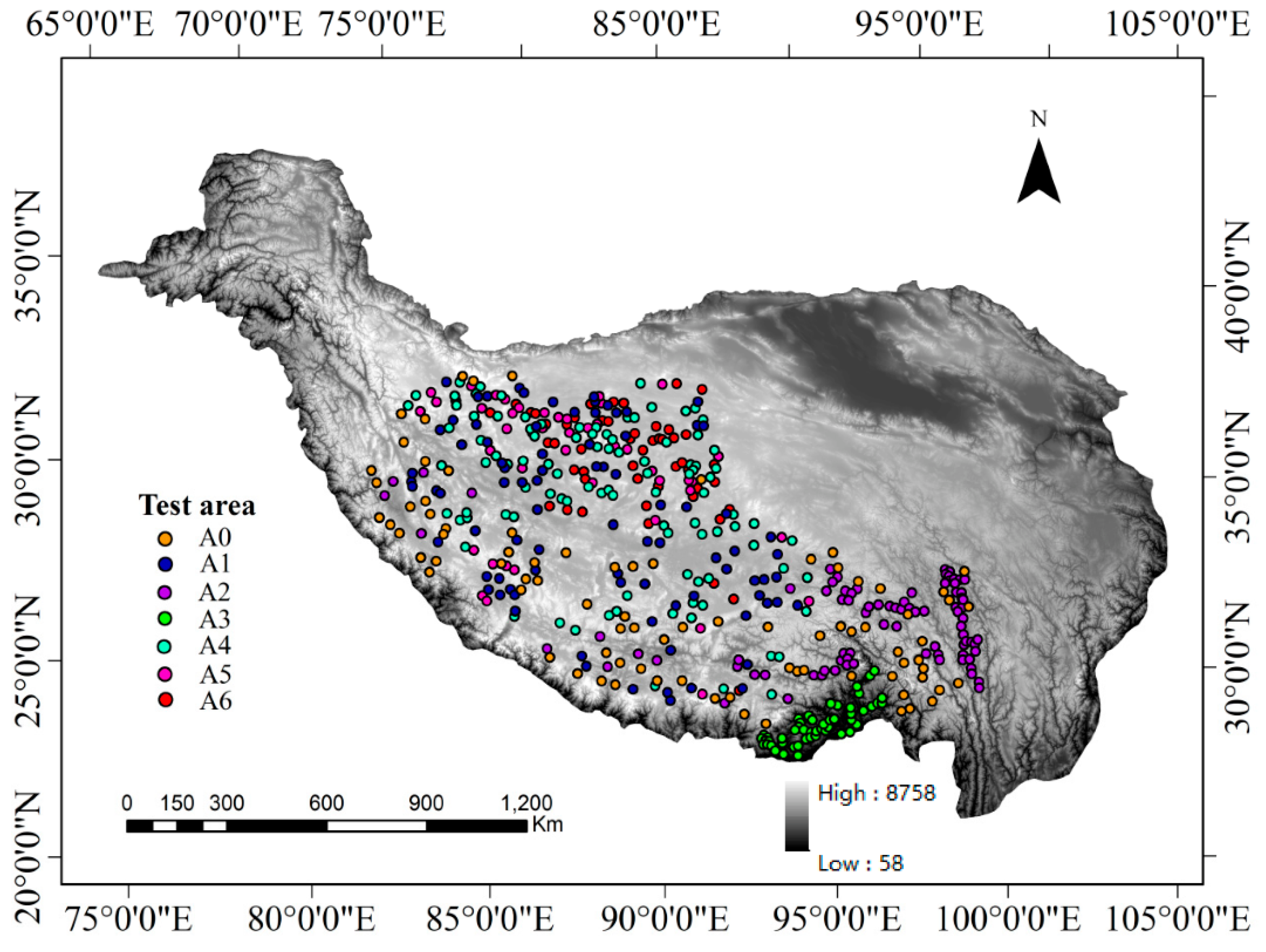
2.1. Study Area and Data
2.2. Methods
2.2.1. Texture Mapping
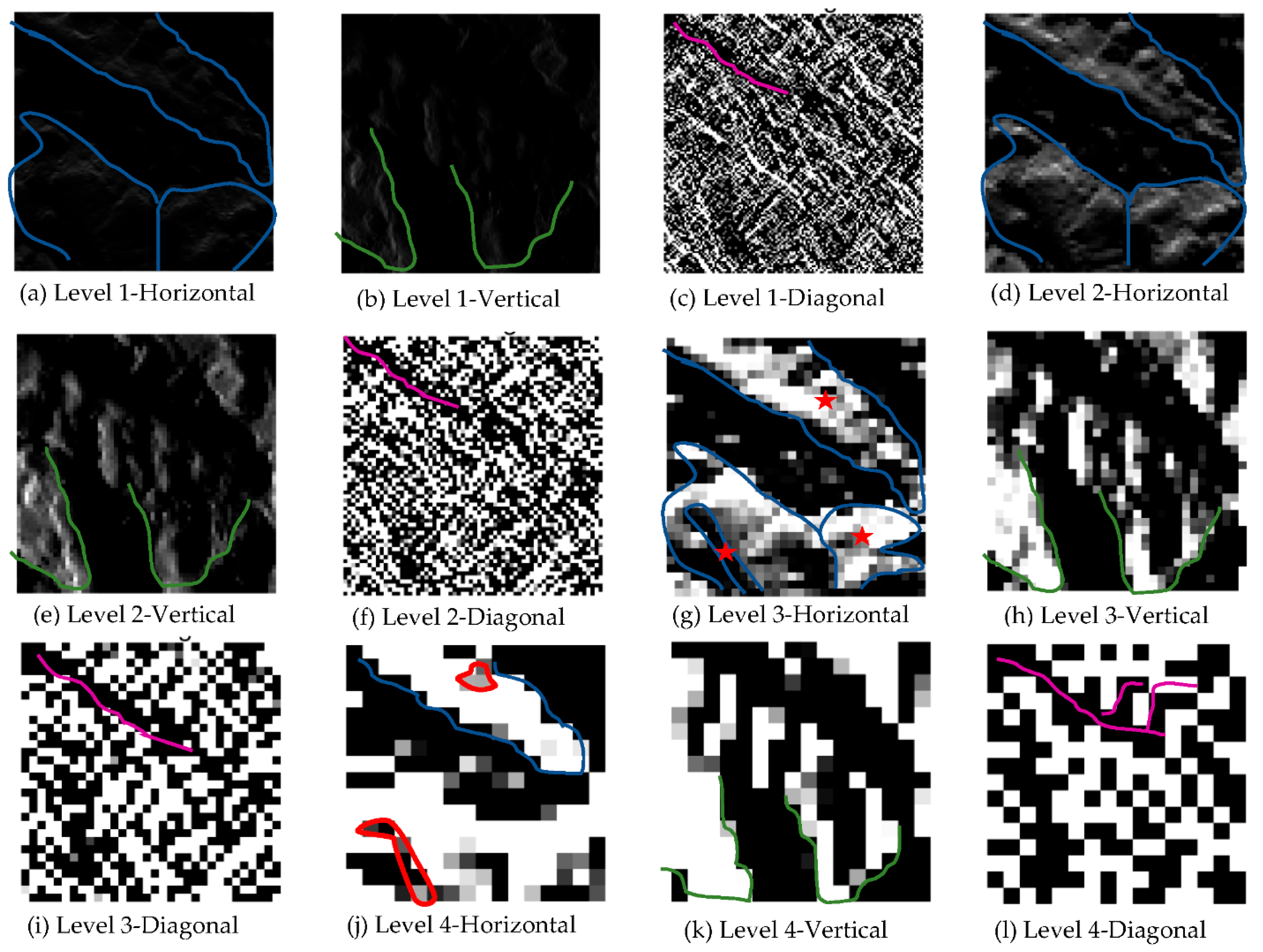
2.2.2. Discrete Wavelet Transform (DWT)
2.2.3. Classification Method of the RF
3. Results
3.1. Determination of Decomposition Scale
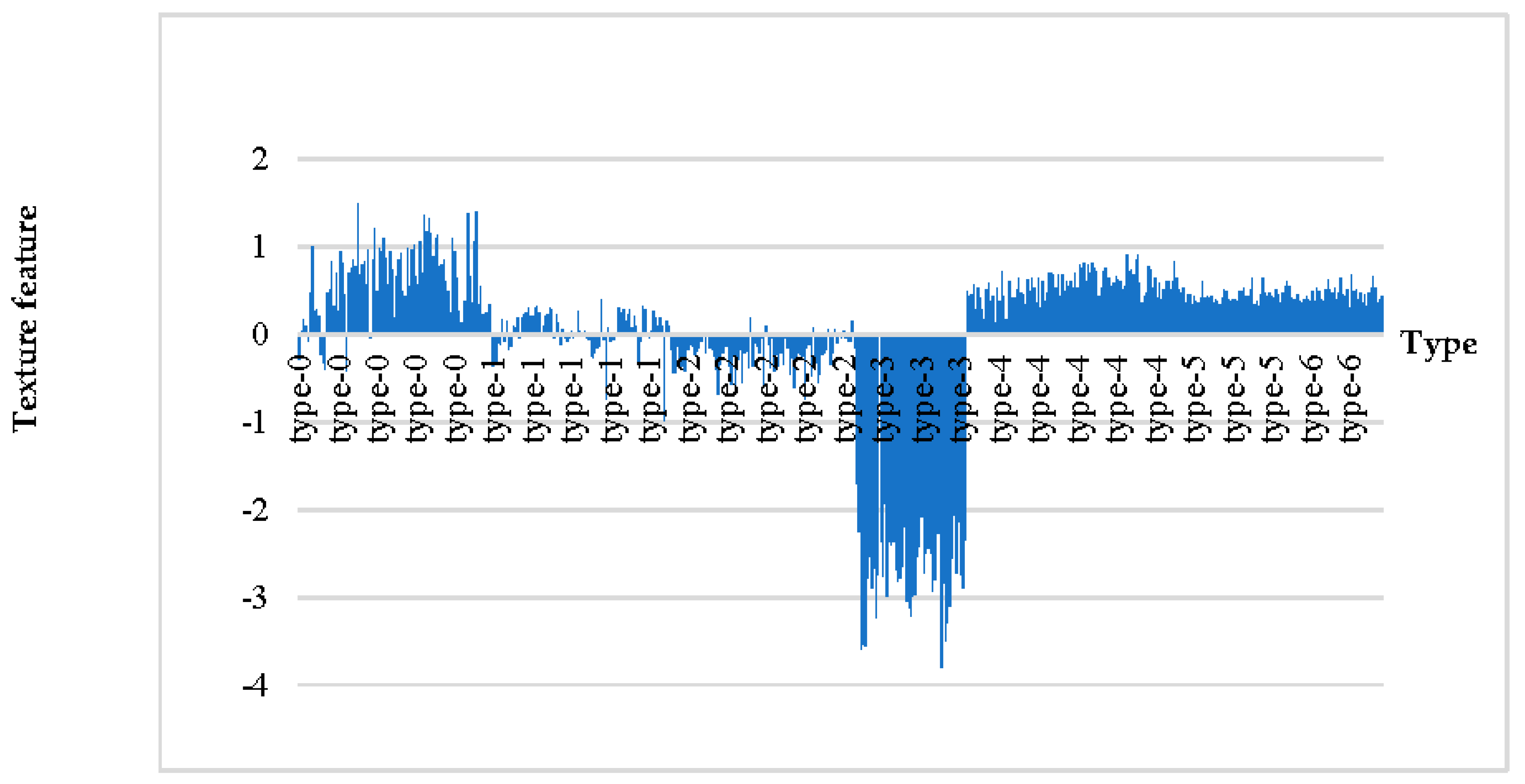
3.2. Extraction of Texture Feature Vectors
3.3. Landform Classification
4. Discussion
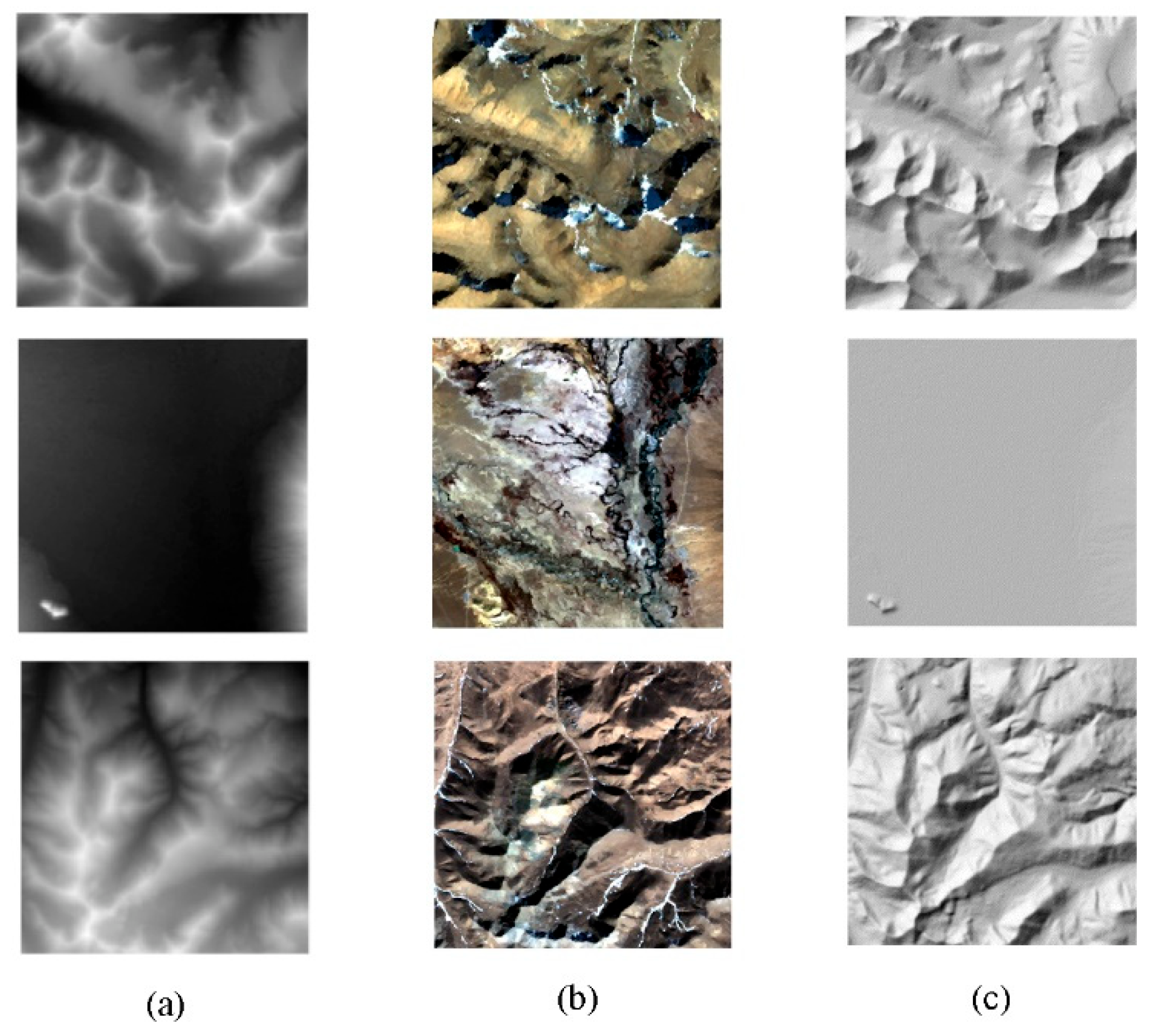
4.1. Comparison of Texture Structure between AW3D30 DEM and ASTER GDEM
4.2. Comparison of Texture Feature Extraction between DWT and GLCM
4.3. Texture Structure Analysis on the Scale Characterization among Different Landforms
4.4. Features Analysis of Landform Spatial Structure Using Different Texture Methods
5. Conclusions
- (1)
- On the basis of the AW3D30 texture image, the DWT method is employed to obtain the local structural features of landforms in low and high frequencies with different decomposition scales. The fine texture structure of a landform is depicted at a low decomposition level. Nevertheless, the coarse texture is stored at a high decomposition level. In the end, the features of the main texture spatial distribution account for the landform direction.
- (2)
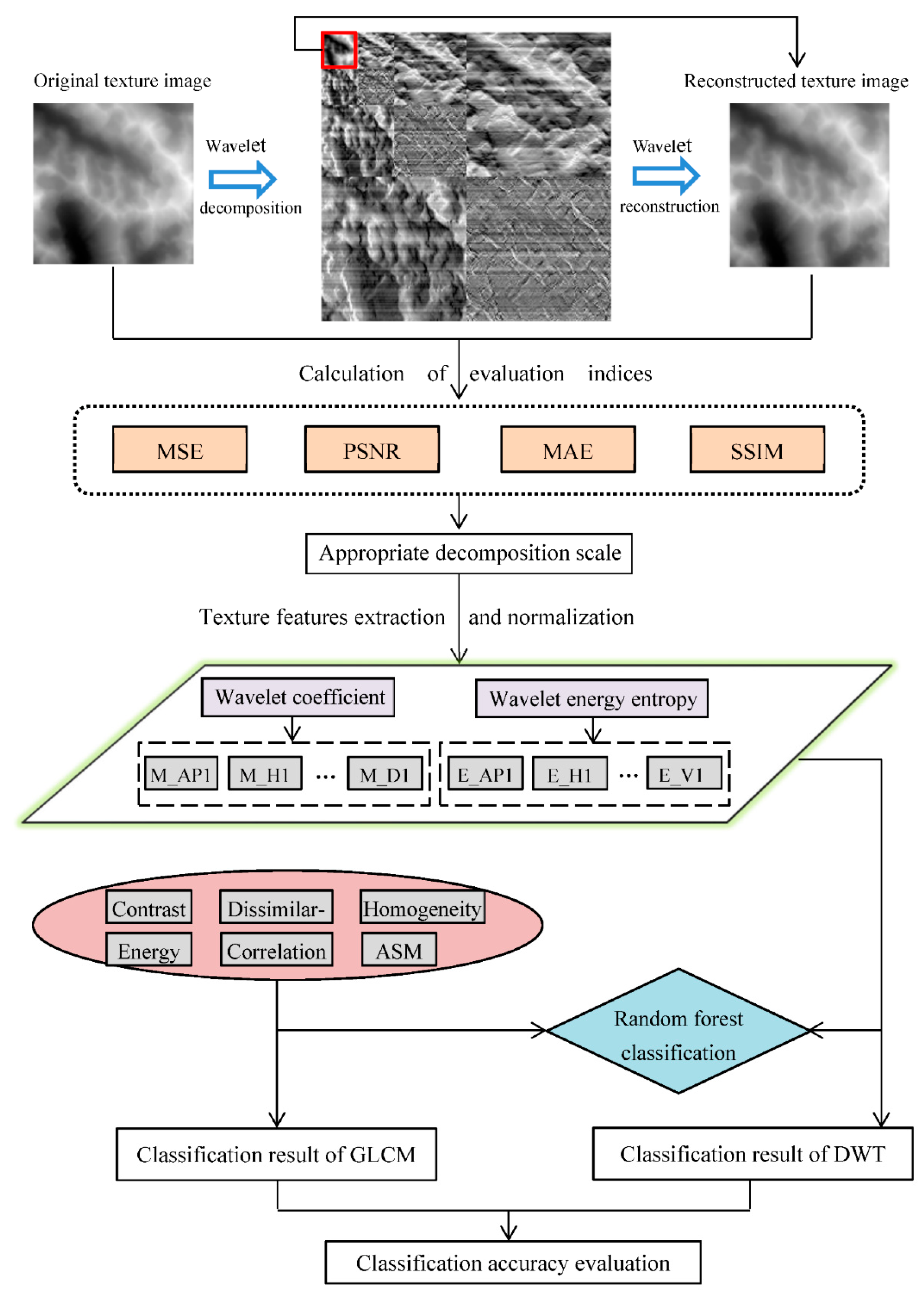
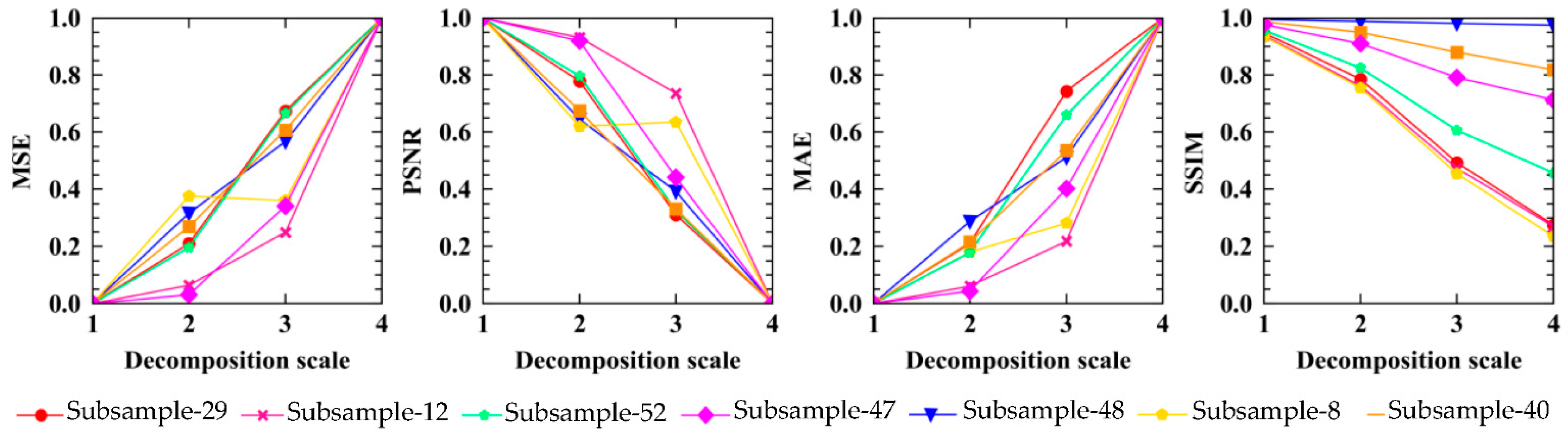
- The appropriate decomposition scale is confirmed using the image evaluation indices of the wavelet reconstruction. Meanwhile, the wavelet coefficients and wavelet energy entropy of the texture are calculated on this scale. Furthermore, the second-order statistical features of six texture measures are extracted using the GLCM method, which makes a full precondition for the landform classification.
- (3)
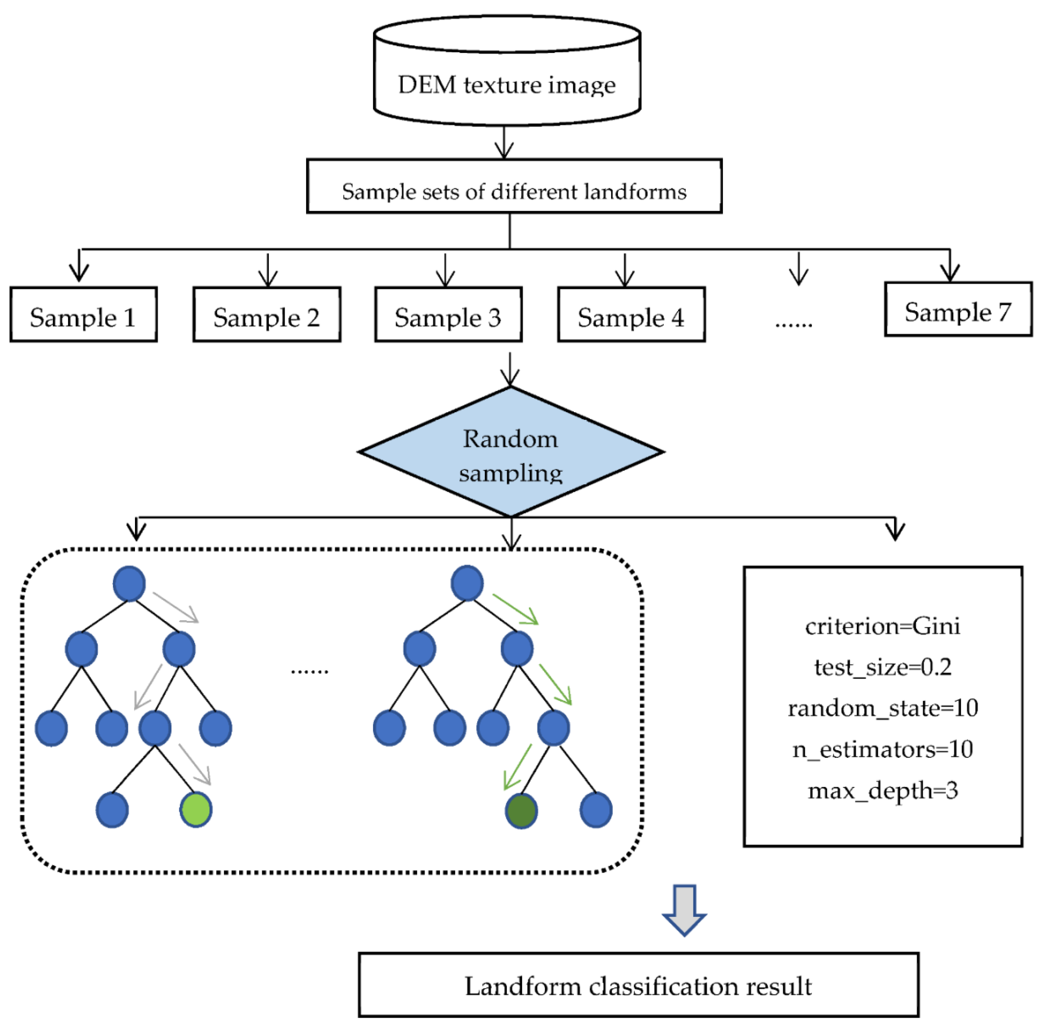
- Given the different texture feature values and the number of samples, the RF method is adopted to classify landforms. Approximately 80% of the total features are selected as training samples to fit the classification model, and the other 20% are used as test samples to evaluate the classification accuracy. The texture method based on DWT, which acquires high classification accuracy with less texture feature dimension, is superior to GLCM in analyzing the gray spatial correlation of the texture structure. A concrete change suggests that the PA of the DWT is increased by more than 67% on A3 (intermediate relief middle mountain), A5 (extremely high altitude plain), and A6 (extremely high altitude high-hill). The overall accuracy was improved by approximately 11.8%.
Author Contributions
Funding
Institutional Review Board Statement
Informed Consent Statement
Data Availability Statement
Acknowledgments
Conflicts of Interest
References
- Pain, C. Mapping of landforms from landsat imagery: An example from eastern new south wales, australia. Remote Sens. Environ. 1985, 17, 55–65. [Google Scholar] [CrossRef]
- Zhang, H.; Zhou, C.; Lv, G.; Wu, Z.; Lu, F.; Wang, J.; Yue, T.; Luo, J.; Ge, Y.; Qin, C. The Connotation and Inher-itance of Geo-information Tupu. J. Geo Inf. Sci. 2020, 22, 653–661. [Google Scholar] [CrossRef]
- Evans, I.S. Geomorphometry and landform mapping: What is a landform? Geomorphology 2012, 137, 94–106. [Google Scholar] [CrossRef]
- Xiong, L.; Tang, G.; Yang, X.; Li, F. Geomorphology-oriented digital terrain analysis: Progress and perspectives. J. Geogr. Sci. 2021, 31, 456–476. [Google Scholar] [CrossRef]
- Liu, K.; Tang, G.; Tao, Y.; Jiang, S. GLCM Based Quantitative Analysis of Terrain Texture from DEMs. J. Geo Inf. Sci. 2012, 14, 751–760. [Google Scholar] [CrossRef]
- Tang, G.; Li, F.; Liu, X.; Long, Y.; Yang, X. Research on the slope spectrum of the Loess Plateau. Sci. China Ser. E Technol. Sci. 2008, 51, 175–185. [Google Scholar] [CrossRef]
- Liu, S.; Li, F.; Jiang, R.; Chang, R.; Liu, W. A Method of Loess Landform Automatic Recognition Based on Slope Spectrum. J. Geo Inf. Sci. 2015, 17, 1234–1242. [Google Scholar] [CrossRef]
- Grohmann, C.H.; Smith, M.J.; Riccomini, C. Multiscale Analysis of Topographic Surface Roughness in the Midland Valley, Scotland. IEEE Trans. Geosci. Remote Sens. 2011, 49, 1200–1213. [Google Scholar] [CrossRef] [Green Version]
- Piloyan, A.; Konecny, M. Semi-Automated Classification of Landform Elements in Armenia Based on SRTM DEM using K-Means Unsupervised Classification. Quaest. Geogr. 2017, 36, 93–103. [Google Scholar] [CrossRef] [Green Version]
- Shang, R.; Peng, P.; Shang, F.; Jiao, L.; Shen, Y.; Stolkin, R. Semantic Segmentation for SAR Image Based on Texture Complexity Analysis and Key Superpixels. Remote Sens. 2020, 12, 2141. [Google Scholar] [CrossRef]
- Trevisani, S.; Rocca, M. MAD: Robust image texture analysis for applications in high resolution geomorphometry. Comput. Geosci. 2015, 81, 78–92. [Google Scholar] [CrossRef]
- Li, B.; Ling, Z.; Zhang, J.; Chen, J.; Wu, Z.; Ni, Y.; Zhao, H. Texture descriptions of lunar surface derived from LOLA data: Kilometer-scale roughness and entropy maps. Planet. Space Sci. 2015, 117, 303–311. [Google Scholar] [CrossRef]
- Iwahashi, J.; Kamiya, I.; Matsuoka, M.; Yamazaki, D. Correction to: Global terrain classification using 280 m DEMs: Segmentation, clustering, and reclassification. Prog. Earth Planet. Sci. 2018, 5, 13. [Google Scholar] [CrossRef] [Green Version]
- Kupidura, P. The Comparison of Different Methods of Texture Analysis for Their Efficacy for Land Use Classification in Satellite Imagery. Remote Sens. 2019, 11, 1233. [Google Scholar] [CrossRef] [Green Version]
- Trevisani, S.; Cavalli, M.; Marchi, L. Surface texture analysis of a high-resolution DTM: Interpreting an alpine basin. Geomorpholory 2012, 161–162, 26–39. [Google Scholar] [CrossRef]
- Iwahashi, J.; Yamazaki, D.; Nakano, T.; Endo, R. Correction to: Classification of topography for ground vulnerability assessment of alluvial plains and mountains of Japan using 30 m DEM. Prog. Earth Planet. Sci. 2021, 8, 1–2. [Google Scholar] [CrossRef]
- Du, L.; You, X.; Li, K.; Meng, L.; Cheng, G.; Xiong, L.; Wang, G. Multi-modal deep learning for landform recognition. ISPRS J. Photogramm. Remote Sens. 2019, 158, 63–75. [Google Scholar] [CrossRef]
- Li, S.; Xiong, L.; Tang, G.; Strobl, J. Deep learning-based approach for landform classification from integrated data sources of digital elevation model and imagery. Geomorphology 2020, 354, 107045. [Google Scholar] [CrossRef]
- Randen, T.; Husøy, J.H. Filtering for texture classification: A comparative study. IEEE Trans. Pattern Anal. Mach. Intell. 1999, 21, 291–310. [Google Scholar] [CrossRef] [Green Version]
- Na, J.; Ding, H.; Zhao, W.; Liu, K.; Tang, G.; Pfeifer, N. Object-based large-scale terrain classification combined with segmentation optimization and terrain features: A case study in China. Trans. GIS 2021. [Google Scholar] [CrossRef]
- Lan, Z.; Liu, Y. Study on Multi-Scale Window Determination for GLCM Texture Description in High-Resolution Remote Sensing Image Geo-Analysis Supported by GIS and Domain Knowledge. ISPRS Int. J. Geo Inf. 2018, 7, 175. [Google Scholar] [CrossRef] [Green Version]
- Haralick, R.M.; Shanmugam, K.; Dinstein, I. Textural Features for Image Classification. IEEE Trans. Syst. Man Cybern. 1973, SMC-3, 610–621. [Google Scholar] [CrossRef] [Green Version]
- Zhao, H.; Fang, X.; Ding, H.; Josef, S.; Xiong, L.; Na, J.; Tang, G. Extraction of Terraces on the Loess Plateau from High-Resolution DEMs and Imagery Utilizing Object-Based Image Analysis. ISPRS Int. J. Geo Inf. 2017, 6, 157. [Google Scholar] [CrossRef] [Green Version]
- Zhao, W.-F.; Xiong, L.-Y.; Ding, H.; Tang, G.-A. Automatic recognition of loess landforms using Random Forest method. J. Mt. Sci. 2017, 14, 885–897. [Google Scholar] [CrossRef]
- Shumack, S.; Hesse, P.; Farebrother, W. Deep learning for dune pattern mapping with the AW3D30 global surface model. Earth Surf. Process. Landf. 2020, 45, 2417–2431. [Google Scholar] [CrossRef]
- Lucieer, A.; Stein, A. Texture-based landform segmentation of LiDAR imagery. Int. J. Appl. Earth Obs. Geoinf. 2005, 6, 261–270. [Google Scholar] [CrossRef]
- Wilhelm, T.; Geis, M.; Püttschneider, J.; Sievernich, T.; Weber, T.; Wohlfarth, K.; Wöhler, C. DoMars16k: A Diverse Dataset for Weakly Supervised Geomorphologic Analysis on Mars. Remote Sens. 2020, 12, 3981. [Google Scholar] [CrossRef]
- Bugnicourt, P.; Guitet, S.; Santos, V.F.; Blanc, L.; Sotta, E.D.; Barbier, N.; Couteron, P. Using textural analysis for regional landform and landscape mapping, Eastern Guiana Shield. Geomorphology 2018, 317, 23–44. [Google Scholar] [CrossRef]
- Wu, J.; Fang, J.; Tian, J. Terrain Representation and Distinguishing Ability of Roughness Algorithms Based on DEM with Different Resolutions. ISPRS Int. J. Geo Inf. 2019, 8, 180. [Google Scholar] [CrossRef] [Green Version]
- Chowdhury, P.R.; Deshmukh, B.; Goswami, A.; Prasad, S.S. Neural Network Based Dunal Landform Mapping from Multispectral Images Using Texture Features. IEEE J. Sel. Top. Appl. Earth Obs. Remote Sens. 2010, 4, 171–184. [Google Scholar] [CrossRef]
- Soille, P. Morphological Image Analysis: Principles and Applications; Springer Science & Business Media: Berlin/Heidelberg, Germany, 2013. [Google Scholar]
- Chellappa, R.; Chatterjee, S. Classification of textures using Gaussian Markov random fields. IEEE Trans. Acoust. Speech Signal Process. 1985, 33, 959–963. [Google Scholar] [CrossRef]
- Aujol, J.-F.; Gilboa, G.; Chan, T.; Osher, S. Structure-Texture Image Decomposition—Modeling, Algorithms, and Parameter Selection. Int. J. Comput. Vis. 2006, 67, 111–136. [Google Scholar] [CrossRef]
- Nikolakopoulos, K.G. Accuracy assessment of ALOS AW3D30 DSM and comparison to ALOS PRISM DSM created with classical photogrammetric techniques. Eur. J. Remote Sens. 2020, 53, 39–52. [Google Scholar] [CrossRef]
- Sun, W.; Wang, R. Fully Convolutional Networks for Semantic Segmentation of Very High Resolution Remotely Sensed Images Combined With DSM. IEEE Geosci. Remote Sens. Lett. 2018, 15, 474–478. [Google Scholar] [CrossRef]
- Gangodagamage, C.; Foufoula-Georgiou, E.; Brumby, S.P.; Chartrand, R.; Koltunov, A.; Liu, D.; Cai, M.; Ustin, S.L. Wavelet-Compressed Representation of Landscapes for Hydrologic and Geomorphologic Applications. IEEE Geosci. Remote Sens. Lett. 2016, 13, 480–484. [Google Scholar] [CrossRef] [Green Version]
- Doglioni, A.; Simeone, V. Geomorphometric analysis based on discrete wavelet transform. Environ. Earth Sci. 2013, 71, 3095–3108. [Google Scholar] [CrossRef]
- Liu, C.; Fang, J.; Liu, Y.; Lu, Y. Field terrain recognition based on extreme learning theory using wavelet and texture features. Adv. Mech. Eng. 2018, 10, 1–10. [Google Scholar] [CrossRef] [Green Version]
- Li, H.; Zhao, J. Evaluation of the Newly Released Worldwide AW3D30 DEM Over Typical Landforms of China Using Two Global DEMs and ICESat/GLAS Data. IEEE J. Sel. Top. Appl. Earth Obs. Remote Sens. 2018, 11, 4430–4440. [Google Scholar] [CrossRef]
- Zhang, G.; Yao, T.; Xie, H.; Kang, S.; Lei, Y. Increased mass over the Tibetan Plateau: From lakes or glaciers? Geophys. Res. Lett. 2013, 40, 2125–2130. [Google Scholar] [CrossRef]
- Zhang, G. Dataset of river basins map over the TP (2016). Natl. Tibet. Plateau Data Cent. 2019. [Google Scholar] [CrossRef]
- Zhao, S.; Cheng, W.; Chai, H.; Qiao, Y. Research on the information extraction method of periglacial geomorphology on the Qinghai-Tibet Plateau based on remote sensing and SRTM: A case study of 1: 1,000,000 Lhasa map sheet(H46). Geogr. Res. 2007, 26, 1175–1185. [Google Scholar] [CrossRef]
- Chang, Z.; Sun, W.; Wang, J.; Zhang, Z. Object-oriented Method Based on Classification of Geomorphic Type in the Tibet Plateau and Adjacent Regions. Mt. Res. 2017, 35, 1–8. [Google Scholar] [CrossRef]
- Zhou, C.; Cheng, W.; Qian, J.; Li, B.; Zhang, B. Research on the Classification System of Digital Land Geomorphology of 1: 1,000,000 in China. J. Geo Inf. Sci. 2009, 11, 707–724. [Google Scholar] [CrossRef]
- Tao, Y.; Wang, C.; Jiang, S. A new method on terrain texture characteristics extraction based on improved dual-tree complex wavelet transform. Geogr. Geo Inf. Sci. 2017, 33, 47–50. [Google Scholar] [CrossRef]
- Karimzadeh, S.; Feizizadeh, B.; Matsuoka, M. DEM-Based Vs30 Map and Terrain Surface Classification in Nationwide Scale—A Case Study in Iran. ISPRS Int. J. Geo Inf. 2019, 8, 537. [Google Scholar] [CrossRef] [Green Version]
- Tadono, T.; Nagai, H.; Ishida, H.; Oda, F.; Naito, S.; Minakawa, K.; Iwamoto, H. Generation of the 30 M-Mesh Global Digital Surface Model by Alos Prism. Int. Arch. Photogramm. Remote Sens. Spat. Inf. Sci. 2016, 41, 157–162. [Google Scholar] [CrossRef] [Green Version]
- Tachikawa, T.; Kaku, M.; Iwasaki, A.; Gesch, D.B.; Oimoen, M.J.; Zhang, Z.; Danielson, J.J.; Krieger, T.; Curtis, B.; Haase, J. ASTER Global Digital Elevation Model Version 2-Summary of Validation Results; NASA: Washington, DC, USA, 2011.
- Su, Z.; Liu, J.; Zhang, L.; Wang, E. Quantifying the late stage topographic evolution of orogenic belts by Fast Fourier Transform spectral analysis: Applications in the Dabie and Micang Shan, China and Sierra Nevada, USA. Chin. J. Geol. 2011, 46, 743–762. [Google Scholar] [CrossRef]
- Arivazhagan, S.; Ganesan, L. Texture classification using wavelet transform. Pattern Recognit. Lett. 2003, 24, 1513–1521. [Google Scholar] [CrossRef]
- Mulcahy, C. Image compression using the Haar wavelet transform. Spelman Sci. Math. J. 1997, 1, 22–31. [Google Scholar]
- Jafarpour, B. Wavelet Reconstruction of Geologic Facies from Nonlinear Dynamic Flow Measurements. IEEE Trans. Geosci. Remote Sens. 2010, 49, 1520–1535. [Google Scholar] [CrossRef]
- Shabou, A.; Baselice, F.; Ferraioli, G. Urban Digital Elevation Model Reconstruction Using Very High Resolution Multichannel InSAR Data. IEEE Trans. Geosci. Remote Sens. 2012, 50, 4748–4758. [Google Scholar] [CrossRef]
- Horé, A.; Ziou, D. Image Quality Metrics: PSNR vs. SSIM. In Proceedings of the 20th International Conference on Pattern Recognition, Istanbul, Turkey, 23–26 August 2010; pp. 2366–2369. [Google Scholar] [CrossRef]
- Wang, Z.; Bovik, A.C. A universal image quality index. IEEE Signal Process. Lett. 2002, 9, 81–84. [Google Scholar] [CrossRef]
- Zhou, W.; Bovik, A.C.; Sheikh, H.R.; Simoncelli, E.P. Image Quality Assessment: From Error Visibility to Structural Similarity. IEEE Trans. Image Process. 2004, 13, 600–612. [Google Scholar] [CrossRef] [Green Version]
- Zhu, J.; Pierskalla, W.P. Applying a weighted random forests method to extract karst sinkholes from LiDAR data. J. Hydrol. 2016, 533, 343–352. [Google Scholar] [CrossRef]
- Phinzi, K.; Abriha, D.; Bertalan, L.; Holb, I.; Szabó, S. Machine Learning for Gully Feature Extraction Based on a Pan-Sharpened Multispectral Image: Multiclass vs. Binary Approach. ISPRS Int. J. Geo Inf. 2020, 9, 252. [Google Scholar] [CrossRef] [Green Version]
- Rodriguez-Galiano, V.F.; Ghimire, B.; Rogan, J.; Chica-Olmo, M.; Rigol-Sanchez, J.P. An assessment of the effectiveness of a random forest classifier for land-cover classification. ISPRS J. Photogramm. Remote Sens. 2012, 67, 93–104. [Google Scholar] [CrossRef]
- Breiman, L. Random forests. Mach. Learn. 2001, 45, 5–32. [Google Scholar] [CrossRef] [Green Version]
- Heung, B.; Bulmer, C.E.; Schmidt, M.G. Predictive soil parent material mapping at a regional-scale: A Random Forest approach. Geoderma 2014, 214–215, 141–154. [Google Scholar] [CrossRef]
- Fu, B.; Wang, Y.; Campbell, A.; Li, Y.; Zhang, B.; Yin, S.; Xing, Z.; Jin, X. Comparison of object-based and pixel-based Random Forest algorithm for wetland vegetation mapping using high spatial resolution GF-1 and SAR data. Ecol. Indic. 2017, 73, 105–117. [Google Scholar] [CrossRef]
- Corcoran, J.M.; Knight, J.F.; Gallant, A.L. Influence of Multi-Source and Multi-Temporal Remotely Sensed and Ancillary Data on the Accuracy of Random Forest Classification of Wetlands in Northern Minnesota. Remote Sens. 2013, 5, 3212–3238. [Google Scholar] [CrossRef] [Green Version]
- Naghibi, S.A.; Hashemi, H.; Berndtsson, R.; Lee, S. Application of extreme gradient boosting and parallel random forest algorithms for assessing groundwater spring potential using DEM-derived factors. J. Hydrol. 2020, 589, 125197. [Google Scholar] [CrossRef]


| Texture Feature Vector | Landform Types | ||||||
|---|---|---|---|---|---|---|---|
| A0 | A1 | A2 | A3 | A4 | A5 | A6 | |
| M_AP1 | 8653.6161 | 9814.7509 | 9476.0397 | 4293.0924 | 10,250.9564 | 10,037.4176 | 10,655.9054 |
| M_H1 | 17,307.2321 | 19,629.5018 | 18,952.0795 | 8586.1848 | 20,501.9129 | 20,074.8353 | 21,311.8109 |
| M_V1 | 34,614.4641 | 39,259.0037 | 37,904.1591 | 17,172.3696 | 41,003.8259 | 40,149.6707 | 42,623.6219 |
| M_D1 | 0.5911 | −0.1545 | 0.9291 | 1.9932 | −0.3359 | 0.1231 | 0.1576 |
| M_AP2 | −1.3961 | −0.1581 | 0.1683 | 0.6722 | 0.0444 | 0.2361 | 0.2982 |
| M_H2 | 0.0037 | −0.0011 | −0.0012 | 0.0144 | 0.0018 | 0.0029 | −0.0013 |
| M_V2 | 2.4643 | −0.6325 | 3.7229 | 7.8841 | −1.3646 | 0.4441 | 0.6453 |
| M_D2 | −5.5351 | −0.6681 | 0.6022 | 2.6728 | 0.1791 | 0.94843 | 1.2391 |
| M_AP3 | 0.0474 | 0.0001 | −0.0261 | 0.0682 | 0.0144 | 0.0078 | −0.0011 |
| M_H3 | 9.0101 | −2.5345 | 14.8371 | 31.4296 | −5.0751 | 1.8197 | 2.6656 |
| M_V3 | −22.0288 | −2.6971 | 2.6118 | 8.5498 | 0.5437 | 3.7606 | 4.6998 |
| M_D3 | 0.1259 | 0.0491 | −0.1794 | 1.2285 | −0.0776 | 0.0008 | −0.2276 |
| E_AP1 | 99.9902 | 99.9999 | 99.9956 | 99.9844 | 99.9993 | 99.9999 | 99.9996 |
| E_H1 | 0.0005 | 0.0001 | 0.0002 | 0.0009 | 0.0001 | 0.0001 | 0.0001 |
| E_V1 | 0.0021 | 0.0001 | 0.0009 | 0.0034 | 0.0001 | 0.0001 | 0.0001 |
| E_AP2 | 99.9908 | 99.9999 | 99.9961 | 99.9873 | 99.9994 | 99.9999 | 99.9994 |
| E_H2 | 0.0005 | 0.0001 | 0.0002 | 0.0008 | 0.0001 | 0.0001 | 0.0001 |
| E_V2 | 0.0018 | 0.0001 | 0.0008 | 0.0028 | 0.0001 | 0.0001 | 0.0001 |
| E_AP3 | 99.9936 | 99.9999 | 99.9957 | 99.9903 | 99.9993 | 99.9998 | 99.9993 |
| E_H3 | 0.0003 | 0.0001 | 0.0002 | 0.0006 | 0.0001 | 0.0001 | 0.0001 |
| E_V3 | 0.0013 | 0.0001 | 0.0009 | 0.0022 | 0.0001 | 0.0001 | 0.0001 |
| Landform Types | Number of Samples | Area/km2 |
|---|---|---|
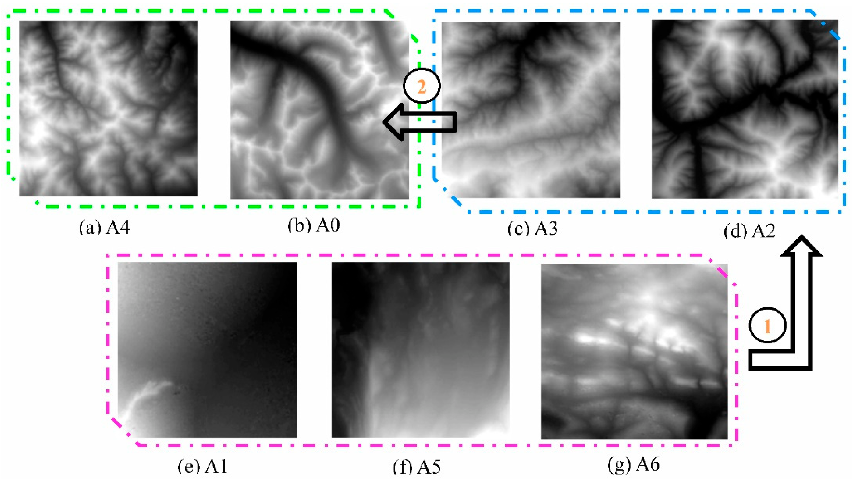
| High relief extremely high altitude mountain (A0) | 85 | 58.9824 |
| High altitude plain (A1) | 86 | 58.9824 |
| Intermediate relief high mountain (A2) | 87 | 58.9824 |
| Intermediate relief middle mountain (A3) | 51 | 58.9824 |
| Low relief extremely high altitude mountain (A4) | 98 | 58.9824 |
| Extremely high altitude plain (A5) | 45 | 58.9824 |
| Extremely high altitude high-hill (A6) | 50 | 58.9824 |
| Texture Analysis Method | Feature Parameter (Extraction Number) | Landform Classification Accuracy (%) |
|---|---|---|
| DWT | Wavelet coefficient (12); Wavelet energy entropy (9) | 91.09 |
| GLCM | Contrast (4); Dissimilarity (4); Homogeneity (4); Energy (4); Correlation (4); ASM (4) | 79.21 |
| Landforms | DWT | GLCM | ||
|---|---|---|---|---|
| PA (%) | UA (%) | PA (%) | UA (%) | |
| A0 | 100 | 100 | 100 | 100 |
| A1 | 94.1 | 94.1 | 100 | 100 |
| A2 | 95 | 100 | 100 | 100 |
| A3 | 100 | 100 | 32.3 | 100 |
| A4 | 83.3 | 88.2 | 100 | 100 |
| A5 | 100 | 77.8 | 0 | 0 |
| A6 | 66.7 | 72.7 | 0 | 0 |
Publisher’s Note: MDPI stays neutral with regard to jurisdictional claims in published maps and institutional affiliations. |
© 2021 by the authors. Licensee MDPI, Basel, Switzerland. This article is an open access article distributed under the terms and conditions of the Creative Commons Attribution (CC BY) license (https://creativecommons.org/licenses/by/4.0/).
Share and Cite
Xu, Y.; Zhang, S.; Li, J.; Liu, H.; Zhu, H. Extracting Terrain Texture Features for Landform Classification Using Wavelet Decomposition. ISPRS Int. J. Geo-Inf. 2021, 10, 658. https://doi.org/10.3390/ijgi10100658
Xu Y, Zhang S, Li J, Liu H, Zhu H. Extracting Terrain Texture Features for Landform Classification Using Wavelet Decomposition. ISPRS International Journal of Geo-Information. 2021; 10(10):658. https://doi.org/10.3390/ijgi10100658
Chicago/Turabian StyleXu, Yuexue, Shengjia Zhang, Jinyu Li, Haiying Liu, and Hongchun Zhu. 2021. "Extracting Terrain Texture Features for Landform Classification Using Wavelet Decomposition" ISPRS International Journal of Geo-Information 10, no. 10: 658. https://doi.org/10.3390/ijgi10100658
APA StyleXu, Y., Zhang, S., Li, J., Liu, H., & Zhu, H. (2021). Extracting Terrain Texture Features for Landform Classification Using Wavelet Decomposition. ISPRS International Journal of Geo-Information, 10(10), 658. https://doi.org/10.3390/ijgi10100658