Towards Managing Visual Pollution: A 3D Isovist and Voxel Approach to Advertisement Billboard Visual Impact Assessment

Abstract

Visual pollution (VP) is a visual landscape quality issue, and its most consistently recognized symptom is an excess of out of home advertising billboards (OOHb). However, the VP related research concerns landscape aesthetic and advertisement cultural context, leaving the impact of outdoor billboard infrastructure on landscape openness unanswered to date. This research aims to assess the visual impact of outdoor billboard infrastructure on landscape openness, precisely the visual volume—a key geometrical quality of a landscape. The method uses 3D isovists and voxels to calculate the visible and obstructed subsets of visible volume. Using two case studies (Lublin City, Poland) and 26 measurement points, it was found that OOHb decreased landscape openness by at least 4% of visible volume; however, the severe impact may concern up to 35% of visual volume. GIS scientists develop the proposed method for policy-makers, and urban planners end users. It is also the very first example of compiling 3D isovists and voxels in ArcGIS Pro software in an easy-to-replicate framework. The research results, accompanied by statistically significant proofs, explain the visual landscape’s fragility and contribute to understanding the VP phenomenon.

1. Introduction

Defining Visual Pollution as Landsacpe’s Quality Issue

Visual pollution (VP) [1], caused by the oversaturation of a landscape with anthropogenic visual information, is a recognized visual landscape quality issue [2] concerning both urban and suburban areas. The above definition provides a general understanding of landscape physiognomy threats and vividly refers to the disharmonious urban features as “pollutants” which we want to get rid of for aesthetic reasons. This research explains that apart from landscape aesthetics, also the geometrical quality of a visual landscape is threatened by the VP, specifically the visible space volume. The research aim is to propose a research method and examine the impact of out of home advertising billboard (OOHb) on landscape openness and triggered the 3D view occlusion effect.

The precise VP definition is still the object of discussion in scientific literature. Furthermore, several research approaches to quantifying the VP phenomenon have been proposed. The VP research aims to assess the landscape’s visual quality and label visually devastated areas as “visual pollution”. The VP assessment can be based on both quantitative [3,4] and qualitative methods relating to subjective public opinions [1,5] or expert knowledge [6]. The factors determining the VP effect are also varied. Some research attributes VP to the visual impact of GSM antennas, street garbage [4] or ill-arranged cables and transmission towers [7]. However, the most common cause of VP are outdoor advertisements (OAs)—the primary medium of the OOHb industry. The spectrum of VP effects is not limited to landscape quality issues only [1,3,8], strengthening its negative assessment as a phenomenon. For example, the OAs’ content, contrasting colors, and graphical layout may induce negative emotions [7] and distract drivers’ attention [9]. Knowledge about the spatial extent and VP level allows local authorities to focus on visually devastated areas [10] and mitigate this unfavorable phenomenon. In the realm of a cityscape, the VP takes advantage of loopholes, resulting in OOHb location in places not intended for it, however efficiently imposing the residents with commercial contents which cannot be switched off. Despite the relatively good recognition of VP in the scientific literature, particularly urban studies and landscape quality-related research, the VP phenomenon needs to be discussed in the context of landscape openness theory [11]. The concepts of landscape openness [12,13,14,15,16] (extensively explained in the Section 2.1) and VP [1] are both well-recognized theories relating to visual landscape quality, which so far have not been put together. Furthermore, monitoring the effect of landscape change on openness is essential for urban planners and policy-makers [17,18]; it applies to VP too. Nevertheless, the mutual relation between landscape openness and VP remains unknown to date. The presented research is an approach to quantifying the impact of VP on landscape openness, precisely the observer’s visible space volume, here measured using 3D ISOVIST.

The objectives of the research are to propose a 3D geographical information system (3D-GIS) based method of outdoor billboard infrastructure visual impact assessment, precisely the impact on landscape openness, and examine the method using a case study OOHb infrastructure spatial configuration. In this paper, the visible volume is referred to using a 3D isovist to a 3D city model created using raster models of topography (2.5D), 3D models of buildings (LoD2) and high vegetation (3D symbols) inlaid with OOHb infrastructure (3D symbols). Based on the above, this work argues that visible volume comparison, calculated in scenarios “with” and “without” OOHb infrastructure, provides quantitative visual impact measures to infer the scope of landscape openness changes. In that sense, the VP problem arises from OOHb infrastructure location, quantity and spatial dimensions, and the resulting impact on geometrical properties of the view volume perceived by the urban space user (the observer).

Furthermore, the view occlusion effect trigged by the OOHb infrastructure is an original contribution to the science of visual impact assessment. The investigation of the OVV verifies whether potentially preferred views have been blocked and to what 3D extent (e.g., vegetation visibility, landmark view). Various OOHb spatial configurations of the same visual volume are not analyzed, although they can be a solution that may reduce VP problems, as emphasized in the discussion section.

2. Literature Review and a Resulting View Volume Concept

2.1. The Impact of VP on Landscape Openness

Landscape openness is a fundamental geometrical parameter of urban space [19]. Hayward and Franklin [11] first considered the concept of landscape openness. They have examined alternative interpretations of organization and characteristics of vertical elements (walls, trees, colonnades) on the perception of open and enclosed space. Presently, the landscape openness concept is being investigated with the use of 3D visibility methods, specifically the 3D Line of Sight (LOS) method [16] and Spatial Openness Index (SOI) [14].

Based on the subjective assessment of analyzed urban forms configurations, a strong correlation between the perceived density and SOI has been proven [14]. Furthermore, it was found that low perceived density contributes to high spatial quality, the same as high spatial openness. The SOI measures the net volume of visible open space in purely geometrical morphological terms; thereby, it can provide a comparative spatial quality evaluation of various spatial configurations [14]. On the other hand, the interdependent landscape enclosure influences the inhabitants’ psychological well-being by attributes such as coherence, safety, relaxation, peace, calmness, and pleasure; therefore, residents prefer less enclosed open spaces [20].

Some OOHb constitute a standalone vertical infrastructure called by Kamicaityte-Virbasiene et al. [21] “a free-standing billboard”. Despite its relatively small size (e.g., the EURO18 standard for is a 6 × 3 m size outdoor billboard infrastructure), such OOHb impacts a cityscape physiognomy, mainly as they are located in the pedestrians’ field of view. All in all, the task of OOHb advertisement is to occupy the pedestrians’ field of view. The outdoor billboard infrastructure is only a part of the city’s advertising landscape, but unlike OOHb, located on building facades, they have a particular impact on perceived landscape openness; however, the assessment of this impact is not yet known. So far, the VP was analyzed with means of 2D [22] and 2.5D [5] visibility, while the use of 3D-GIS visibility may spotlight cityscape openness—the visible space volume. Hence, the hypothesis that outdoor advertising vertical infrastructure impacts the landscape openness significantly contributes to visible and not visible view volume imbalance. The scale and extent of this impact have not been examined to date, and it is being considered a contribution to visual impact assessment methods.

2.2. The Advantages and Limitations of 3D-GIS Visibility in Landscape Studies

Since 1979, when Benedikt proposed isovist [23] and Felleman calculated viewshed [24], visibility analysis has been the core function of GIS software. The main differences between the viewshed and the isovist are that the first method uses a raster of a digital surface model for visible terrain calculations; therefore, it is preferred in landscape studies at a small scale. The isovist relies on vector data and measures the area, perimeter, occlusivity, and variance skewness of the isovist field, meeting architecture and urban space research expectations. However, both methods are not assigned to any research area, both analyzing the visibility field specifically. Isovist is a set of visible points from a given point [25], viewshed is a set of visible cells [24], the pixels. Visibility calculation algorithms have made GIS visibility maps the essential tool of visual impact assessment frameworks [26]. However, the 2D viewshed model does not always meet the expectations in terms of visibility accuracy. As proven by Sahraoui et al., [27], the 2D viewshed results in an overestimated visible area compared to the tangential view (2.5D) viewshed. Higher accuracy is expected as the added value of 3D visibility analysis, despite the need for higher computer processing power to achieve it [28].

The development of GIS software also influenced the visual impact assessment methodologies, which moved on from 2D visible area measurement to 3D visual sphere [29] to reflect the complex nature of visibility with more details and accuracy. For example, the sky view factor basically investigates the impact of urban forms on urban heat islands [30]; in practice, it measures the fraction of visible sky sphere [31,32] occluded by urban features. The building view factor [33] quantifies the sole impact of buildings on the urban radiative balance. The sky view factor analysis, formerly used in the energy-related analysis [34], has inspired Yang to implement the sphere concept of visibility analysis, namely a “viewsphere”—the visible volume that is filled with the ambient optic array [29]. The viewsphere concept is recognized in urban configuration studies [35,36], alternatively referenced as a visual bowl [37]. The measure of visible volume is successfully used in the 3D study of visual change and quantification of the visual impact of proposed building development so far. However, the above 3D-GIS approaches are based on the skyline, specifically the skyline barrier analysis [38,39]. The skyline barrier analysis is subject to specific technical limitations, and it is not intended to analyze the visual impact of objects lower than the surrounding buildings. To exemplify, if the analyzed urban feature is located on a sightline between an observer and tall buildings and does not intersect the skyline, it is omitted in skyline barrier analysis. Thus, its impact on the visual volume will stay uncharted. This situation also applies to OOHb infrastructure, which is usually located against the background of buildings and does not intersect the skyline. Perhaps small urban features do not have visual impact significant enough to be the object of 3D visual impact assessment studies, but this is not the VP case. A kind of ray-tracing approach is needed here to assess the viewing volume change concerning the buildings outlined by the skyline.

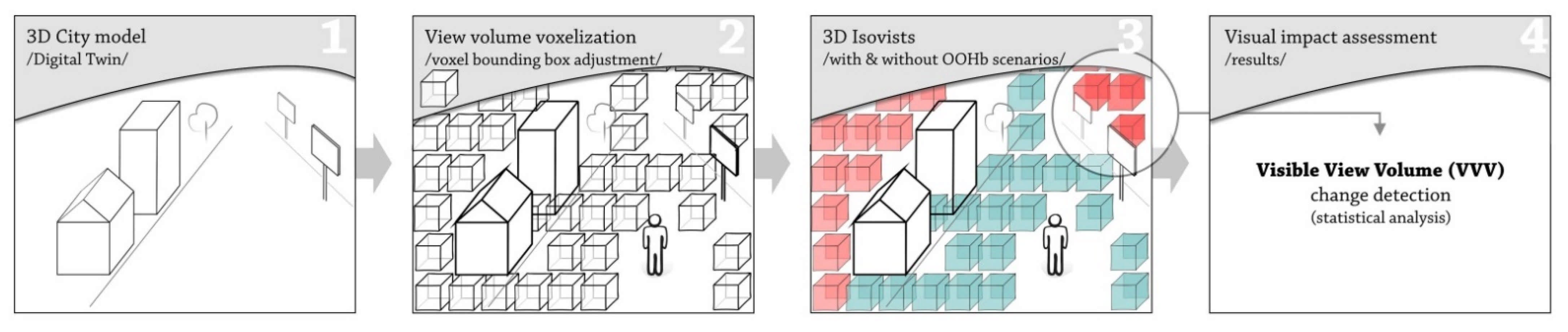
2.3. The View Volume Concept

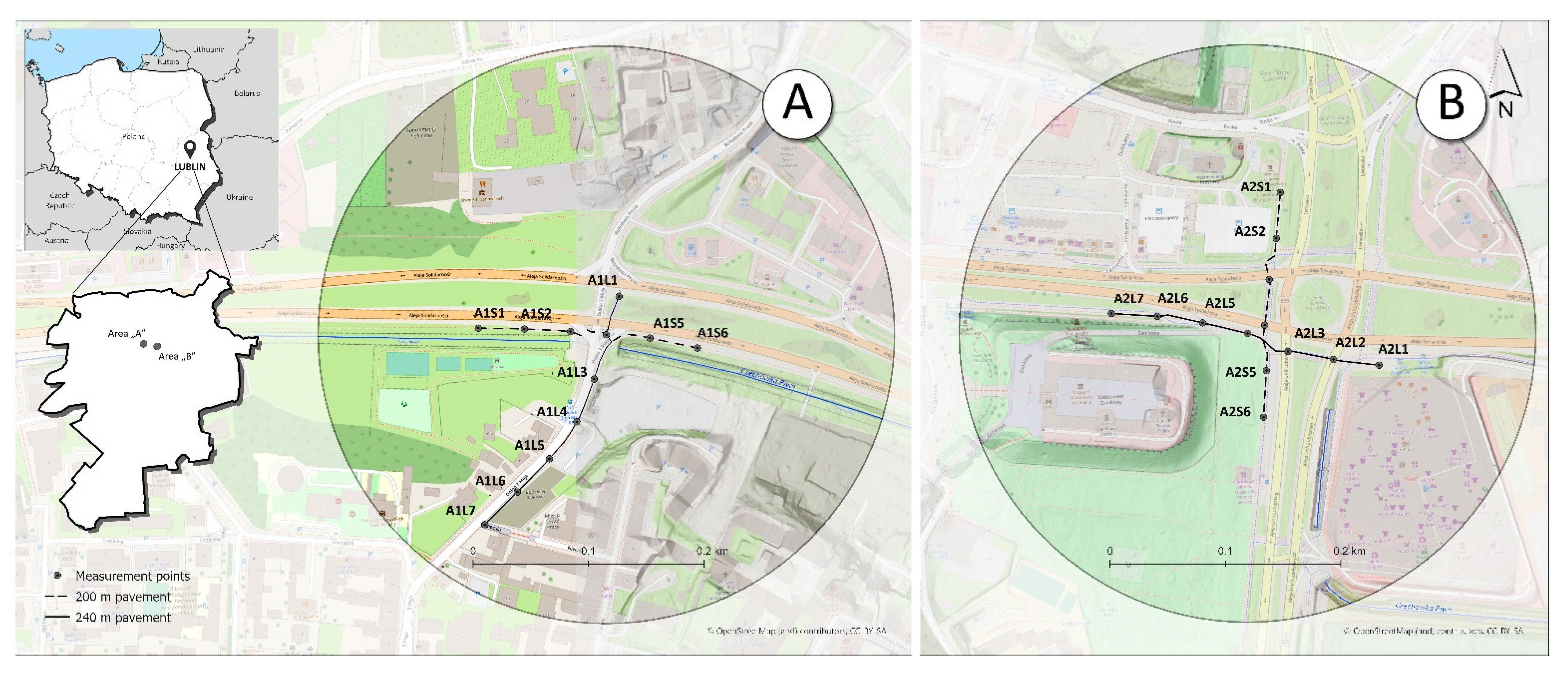
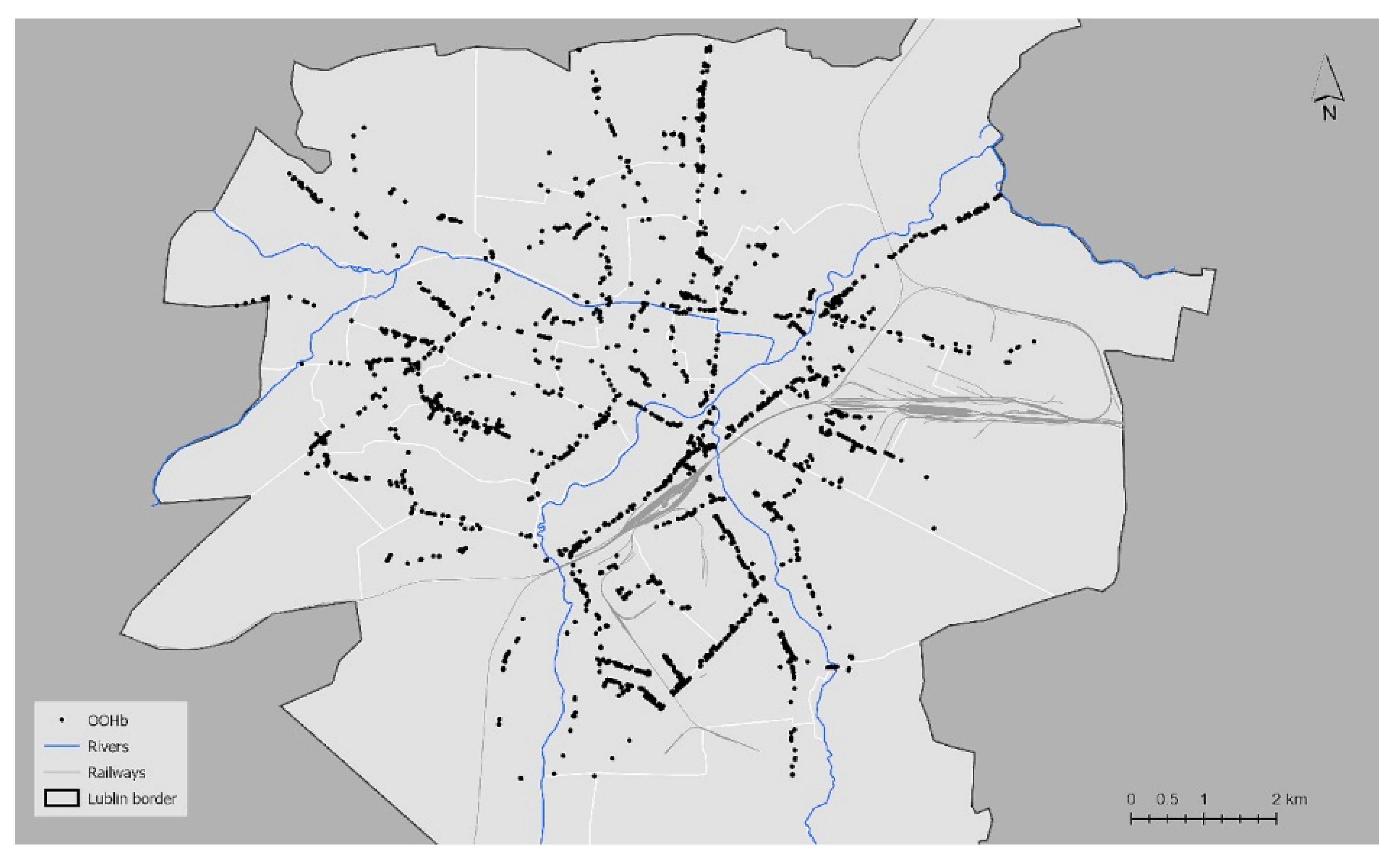
The aforementioned skyline barrier limitations [39] have been overcome with voxels and 3D Isovist analysis in this study. Furthermore, the “viewsphere” concept is not emphasized here in favor of the term “view volume” and 3D bounding box as a consequence of using voxels (Figure 1). The view volume refers to viewing capabilities of the observer. It contains two subsets: the visible view volume (VVV), referring to the visible part of the view volume (the blue in Figure 1), and the obstructed view volume (OVV), which refers to the not visible part of the view volume (the red color in Figure 1). Both parameters are interdependent, and their sum is equal to view volume. Some research uses similar terminology, emphasizing the “sphere” instead of “volume” as the 3D field of view is based on the 3D sphere. The voxels bounding box, which determines the 3D extent of the analysis, does not correspond with the sphere. Therefore, it is not used in this study, although it can be trimmed to it.

Notably, the OVV points out the occlusion effect to make the public space users and local urban planning authorities aware of “what will be taken from” instead of “how much will be added to” their view. Batty argued the enclosed space measurement is a crucial issue of good urban design development [25]. This work similarly argues that VVV–OVV balance makes the VP assessment frameworks more specific as both visible and occluded parts of the view volume are analyzed. The above reveals the visual losses due to the location of the OOHb infrastructures.

3. Case Study

The VP is sometimes called “the billboardization” [40], as shown by the scientific literature concerning many countries [41,42,43,44] also post-communist regions, which during socio-economic transformation left the landscape quality issues unattended. This study takes Lublin City (Poland) as an example of spatial planning neglect and a VP method testing case study. As part of the author’s research, in 2015, a field inventory of Lublins’ advertising media was made, resulting in the advertisement billboard location map presented in Figure 2.

The field inventory method was described in [5], the total number of 3426 advertisement billboards’ locations have been recorded along the main roads of Lublin City. The created outdoor advertisement GIS database is not an official register (such register is not required from the Polish city surveying services); however, it allows distinguishing the places of VP concentrations within the city of Lublin. The OOHb infrastructure is mainly located along main roads or around crossroads, usually distanced from the buildings. The selection of specific sites (case studies areas) of the VVV–OVV method testing was made according to the following conditions:

• Presence of the OOHb infrastructure among other forms of outdoor advertising
• Heavy pedestrian traffic—herein, the visual impact of OOHb infrastructure is being considered from a pedestrian observer perspective, and the window view is not the object of analysis (e.g., car drivers, house dwellers)
• A relatively isolated OOHb spot—to avoid the spillover effect of neighbour advertisement media.
• Non-flat area—to demonstrate the usability of the method at various topography conditions.

Knowing the spatial characteristics of the VP of Lublin City, two case study areas were selected: the 3-Maja St. and the Solidarności Av. crossroads (Area A) and the Solidarności Av. and the Unii Lubelskiej Av. crossroads (Area B). Both cases study areas were located along the Solidarności Av. and distanced 1 km from each other. For results visualization and database management, they were clipped to 1000 m side squares. Both case study areas cover the Czechówka river valley, which determine a varied topography (Figure 3A,B). The elevation above sea level is ranging from 168.8 to 206.3 m for area A and 165.7–198.9 area B, respectively. The Solidarności Avenue is one of the leading transport alterations of the city, where intensive pedestrian traffic is generated by a bus station, market and a shopping mall, as well as tourist attractions of the Old Town Lublin. Therefore, a set of measurement points were proposed for both case study areas. Measurement points were equally spaced (40 m) along “short” (200 m) and “long” (240 m) pedestrian patches digitized in N–S and E–W directions. For the above described case study landscapes, the 3D-city model was created according to the method procedure described in the next section.

4. Method Section

The research method basically consists of four steps: the digital twin creation using 3D geospatial data (described in Section 4.1), the voxels size (resolution) adjustment and view volume voxelization (Section 4.2), essential visibility analysis using the 3D Isovist method (Section 4.3) and the statistical analysis of detected VVV changes and visual impact interpretation. The method workflow is presented in Figure 4.

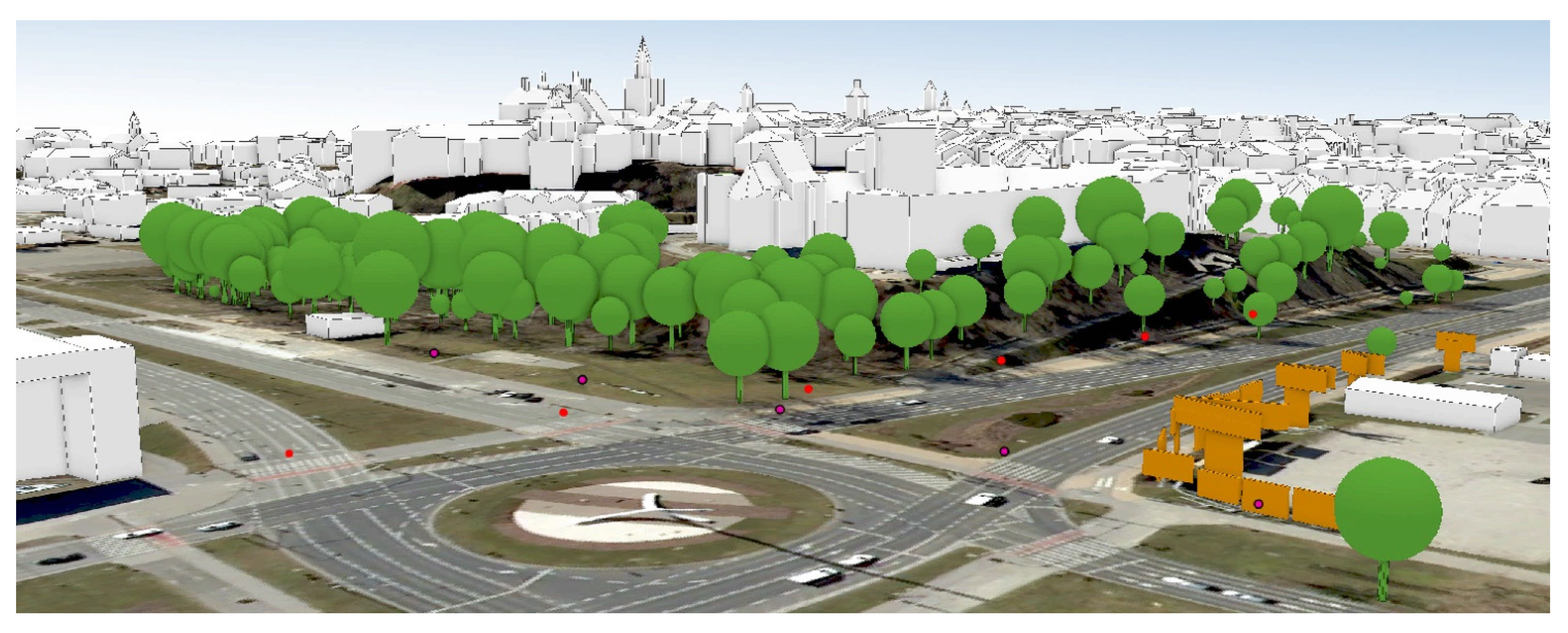
4.1. The Method of 3D City Model Creation

The research method uses the 3D isovist to measure the visible and obstructed volume of the cityscape; therefore, it was necessary to create a 3D city model first. Purposely, the well-recognized GIS software (the ArcGIS Pro v. 2.8) has been used to open the method to urban issues community without using external plug-ins or programming languages. The above enhances the method repeatability; on the other hand, it imposes a geoprocessing framework. Furthermore, open geospatial data from the Polish national geoportal repository were primarily used to create the model [45]. These datasets include a 3D point cloud, 3D building model and orthophoto image. The 3D point cloud was acquired in 2017 using aerial LiDAR and classified according to LAS 1.2 specification [46]. The 3D point cloud density was 12 points/m², and the mean point spacing was 0.22 m, which enabled the digital elevation model (DTM) raster extraction at 0.5 m ground sample distance (GDS). To improve the 3D city model, the natural color composition orthophoto image was added to the 3D scene (image acquired March 2020 and shared via geoportal as tiff files at 0.25 m GSD). The 3D building model was downloaded in GML format at the second level of details (LoD2) (file section no. 0663) and converted to multipatch format accepted by ArcGIS Pro software. The 3D building model was 2011 dated, it requires minor updates, herein with the means of manual building solid editing, using 3D point cloud as references. The 3D city model was completed with a high vegetation layer (trees). Trees were symbolized using the 3D tree symbol library of ArcGIS Pro software, the tree trunks’ location and height parameters were approximated using a local maxima of rasterized canopy height model [47]. The last but not least layer used for 3D city model creation was the 3D symbol of OOHb infrastructure. Basically, the author prepared this layer using a profile view of the 3D point cloud, enabling the OOHb infrastructure location and size measurement (Figure 5A). From a technical point of view, the billboard’s upper edge was first digitized as a 2D line using a digital surface model (DSM). The DSM was extracted from classes 1 and 2 of the 3D point cloud and saved at 0.3 m GSD (Figure 5B). Next, the length of the digitized line measures the advertising board length (L). Next, the line was buffered (diameter 0.25 m) and extruded in 3D view as 0.25 m width (W) rectangles, with adopted 3 m height (H) parameter. Finally, the adopted 3 m H parameter was adjusted to its actual dimension and elevation above ground level using a profile view of the 3D point cloud (Figure 5B). The 3D symbols of OOHb were saved as multipatch objects and used for 3D city model visualization and further isovists calculations.

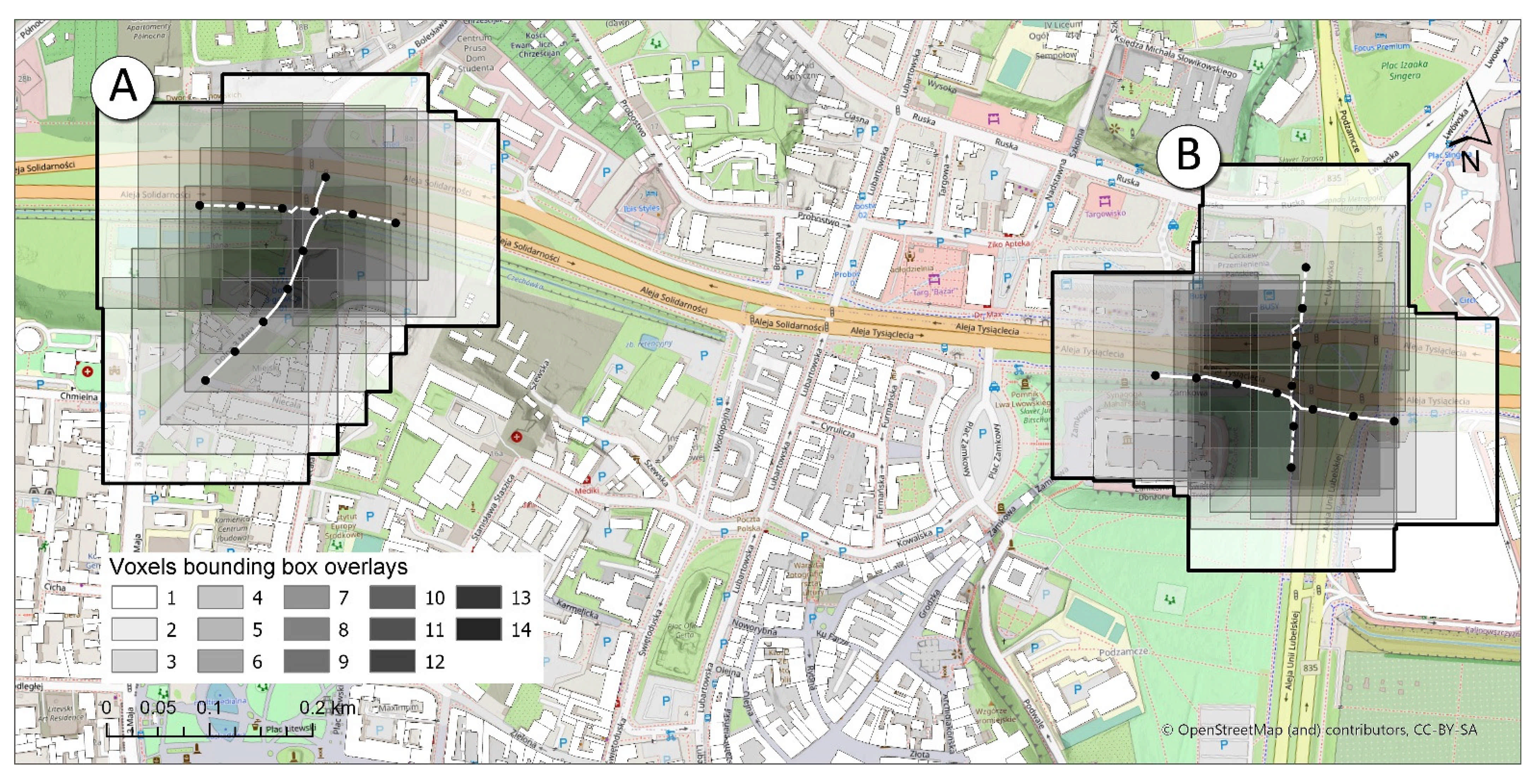
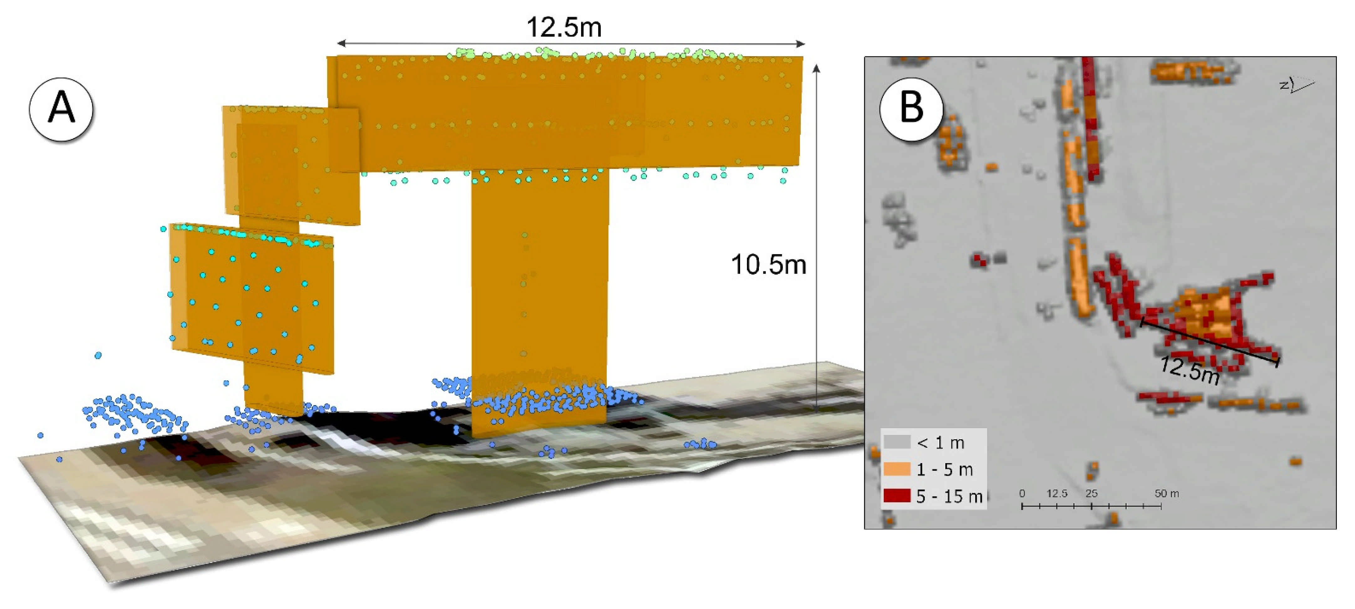
4.2. Filling Up the Bounding Box with the Voxels

A voxel describes the smallest distinguishable cubic part of a 3D object. Since 1979 [48], the voxels application has spread from medical imaging (specifically the computer tomography) to other fields of science, including urban studies [37,49], however not without technical limitations, which applies to this research method too. Basically, the smaller the voxel, the finer detailed analysis that can be conducted, but it comes with a high computer processing power demand. Hence, the voxel size optimization experiment was set up at the outset and aimed to find the voxel size to provide the exact result without slowing down the geoprocessing. The literature review suggests that 1 m voxel size can be an optimal parameter for 3D feature voxelization [28,50], however, these guidelines do not apply to fill up the bounding box with the voxels which is the case of this method. Therefore, several 3D isovists analyses were run each time, splitting voxels into four equal boxes to answer the optimal voxel size question and adjust the bounding-box 3D extent. As a starting point, a rough 10 m voxel has been used and next downsampled to 5, 2.5 and 1.25 m.

Moreover, it was also expected that 3D isovist computation time would not exceed 1 h. The above assumptions were tested on 200 × 200 and 40 m (length, width, height) voxel bounding box. The bounding box length and width dimensions correspond to the foreground visibility range recommendations proposed by Palmer [51] as well as other visibility simulation experiments [52], the height of the bounding box corresponds to the difference in height between the observer’s point and the highest building of the case study. The experiment was set up using a single measurement point located in the center of the bottom of the bounding box and elevated 1.7 m above ground level to reflect the mean eye height of the pedestrian observer. The results in VVV and OVV discrepancy resulting from tested voxel sizes and the computation time were summarized in tables and discussed in terms of optimal for a case studies 3D ISOVISTS parameters

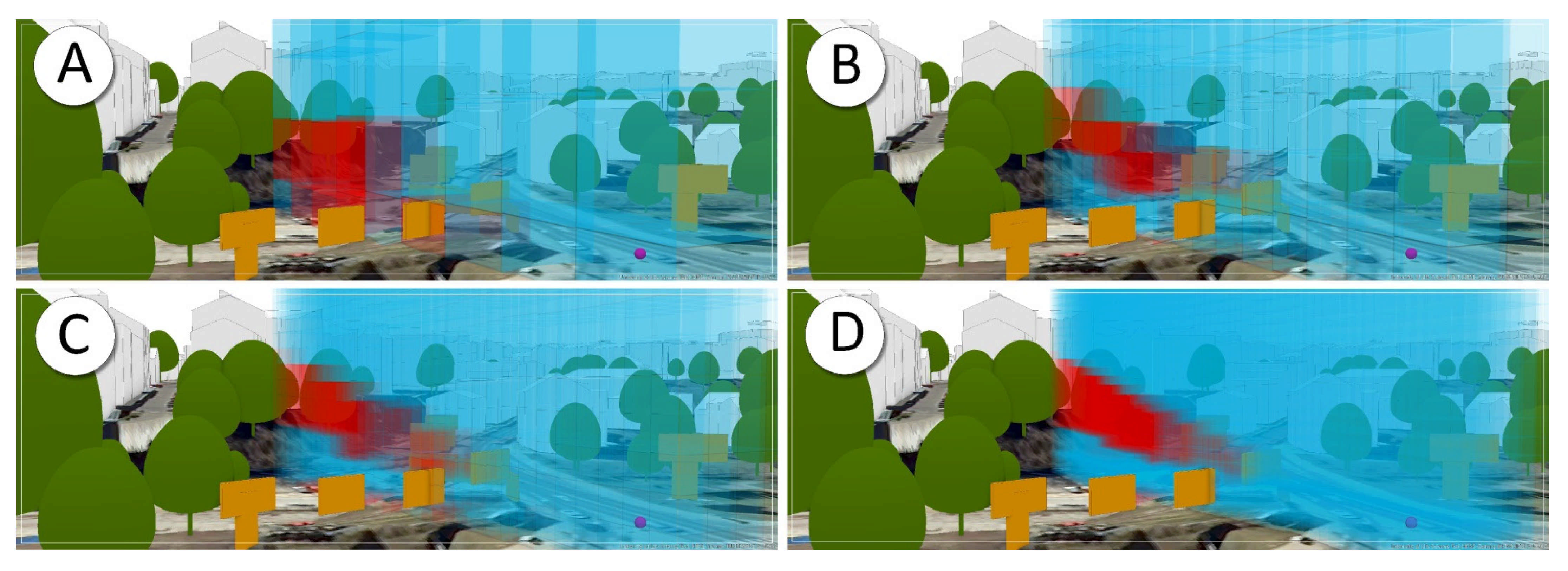
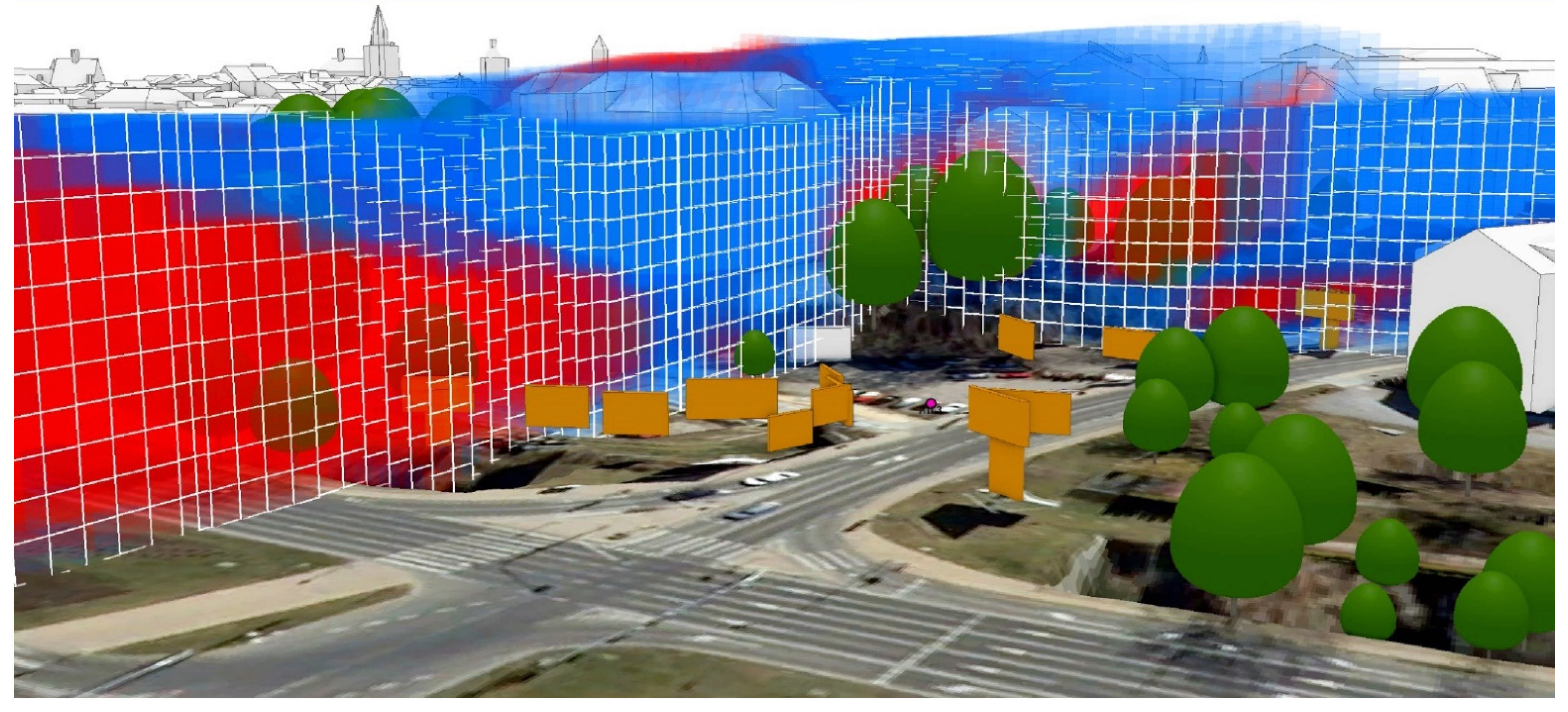
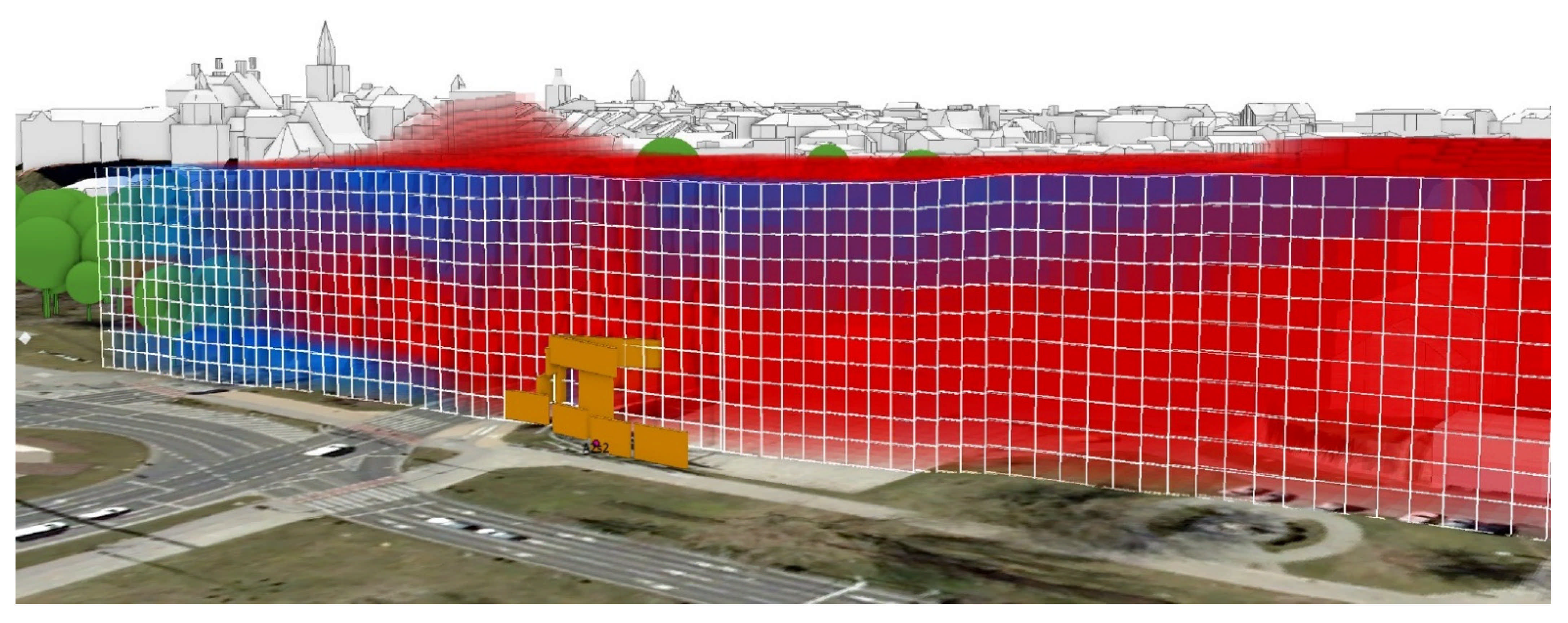
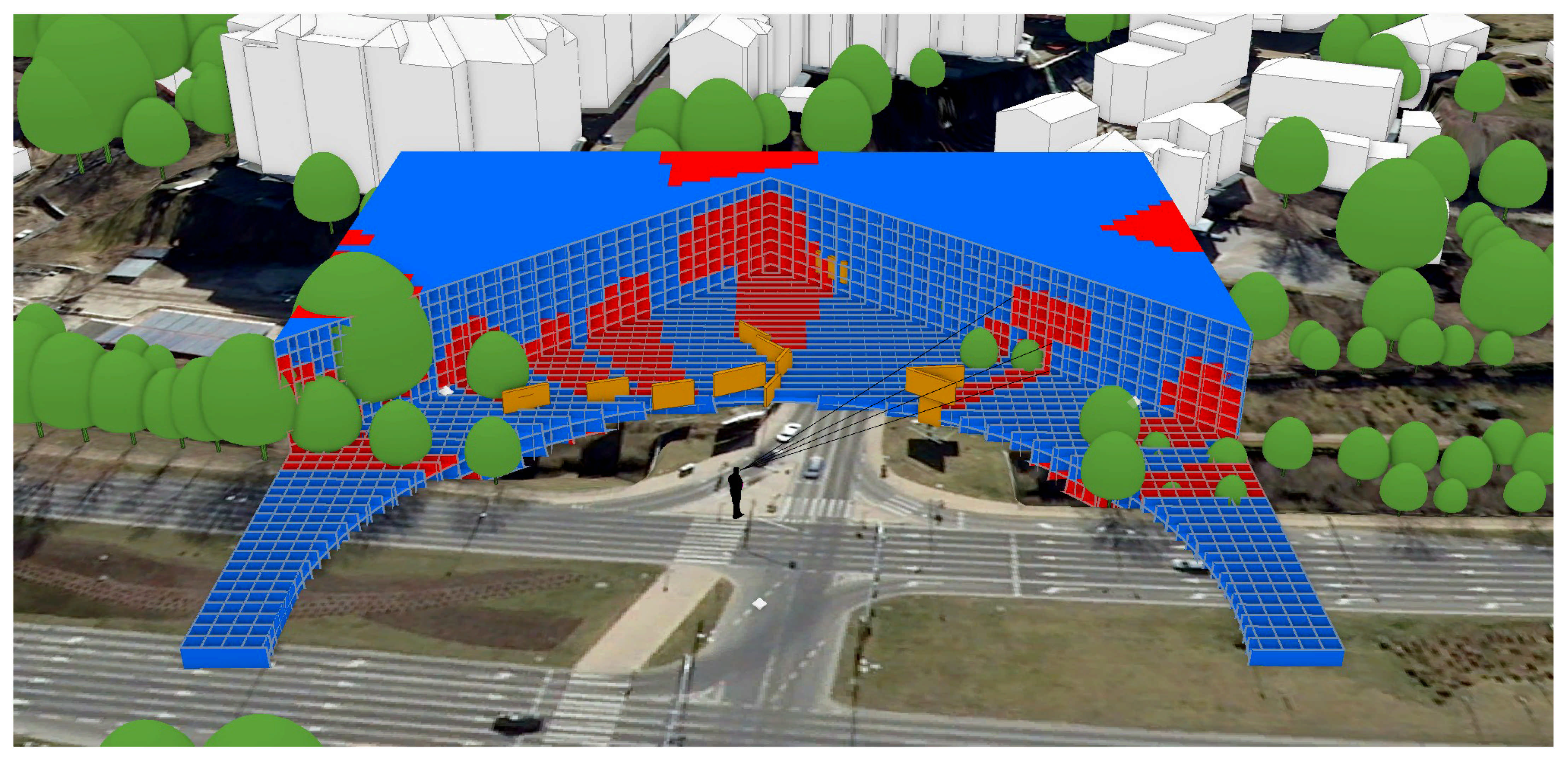
4.3. Solving 3D Isovists Using Voxels

The ArcGIS Pro software does not provide a tool for isovists instantly. To perform the 3D isovist analysis, the sightlines were constructed between the measurement point and the voxels. The line of sight analysis divides sightlines into visible and obstructed sections; thus, the visibility status of the sightlines section connected with the voxel was assigned to the voxel. By summarizing the visible and not visible voxel volume, the VVV and OVV parameters were calculated, respectively. The visible voxels were visualized in blue and coded using VisCode = 1, and the obstructed voxels were visualized in red with assigned VisCode = 2. The profile view was used to explore the bounding box insides. The computing was carried out on the CREODIAS Virtual Machine with the following resources: the ArcGIS Pro software (v 2.7); 12vCores, RAM 117 GB, local disc 128 GB, GPU RTX2080TI.

4.4. The 3D ISOVISTS Scenarios and Statistical Analysis Method

To measure the impact of OOHb infrastructure on the VVV–OVV balance, the 3D ISOVIST was repeated twice, first using the DTM, LoD2 and 3D trees symbols as visibility curtains, secondly, also taking into account the OOHb 3D symbols. Such “OOHb-free” and “OOHb” scenarios were executed for all 26 measurement points along with the measurement patches of each case study area. In total, 52 ISOVISTS were planned (26 for “OOHb-free” and 26 for “OOHb” scenarios). Importantly, each measuring point has an individual voxel bounding box. For example, the measurement point 40 m spacing caused the voxel bounding boxes overlapping effects illustrated in Figure 6.

The VVV and OVV were compared using graphs and basic statistics measures (median, minimum, maximum, first and third quartile). To measure the statistical significance between “OOHb-free” and “OOHb” scenarios, the Sign test and Wilcoxon non-parametric test at a p-value of 0.05 was used. The Statistica (v 13.3) software was used for the above calculations.

5. Results

5.1. 3D City Modelling

A total of 67 OOHb objects have been measured and converted into 3D symbols, 33 in area “A” and 34 in area “B”. Advertisements were located along main roads to catch both passersby and drivers’ attention. The created 3D city model was supplied with 759 tree symbols, 461 in area “A” and 298 in “B”, tree height ranging from 3 to 28 m. In total, 44 new buildings have been updated at LoD2. Above 3D layers were the object of visualization in ArcGIS Pro local scene, presented in Figure 7.

5.2. The Results of Voxel Sizes Testing

Four 3D ISOVIST tests were completed, each time using four times smaller voxels to assess the impact of its size and number on resulting VVV and OVV values as well as computation processing power demand. The total volume of the voxels bounding box used in pre-tests was 2,000,000 m³, as the volume of the voxel decreased (ranged from 1000 to 1.953125 m³), the number of voxels filling up the bounding box volume increased 512 times (

Table 1. The pre-test results on optimal voxel size.

Voxel Size (m)	Voxel Volume (m3)	Voxels in b.box	Visible Voxels	Obstructed Voxels	Visible Voxels (%)	Obstructed Voxels (%)	VVV (m3)	OVV (m3)	Computation Time (min, s)	Post-Processing Time (min)
10	1000	2000	1599	401	80.0	20.0	1,599,000.0	401,000.0	0; 42	On the fly
5	125	16,000	12,247	3753	76.5	23.5	1,530,875.0	469,125.0	2; 37	On the fly
2.5	15.625	128,000	107,836	20,164	84.2	15.8	1,684,937.5	315,062.5	21; 2	3–4
1.25	1.953125	1,024,000	881,922	142,078	86.1	13.9	1,722,503.9	277,496.1	75; 34	74

). The significant increase in the amount of data to be processed goes with computation time up to 2 h. Moreover, in the case of the finest voxel size (1.25 m), additional time was required by the system to assign the visibility status of the sightline to the voxels, as well as to save the edits (so-called post-processing time). The conducted test revealed a significant increase in analysis execution time due to voxels size decrease, thus increasing analysis 3D resolution. It turns out that the most coarse voxel (10 m) resulted in 6.1% worse results, about 1.25 m voxels. The finer the voxel size, the smaller proportion of OVV was in the viewed volume (Figure 8). Smaller voxels reflect the 3D shape of the viewing curtain better; therefore, it is reflected by a lower OVV value. The long computation at 1.25 m voxels and relatively worse results at 5 m voxel (herein interpreted as outliers), the 2.5 m voxels, were chosen for further processing. Moreover, the bounding box height parameter was reduced from 40 m to 25 m to reflect the neighboring building background better (the 40 m occurs to overestimate the VVV by measuring the viewing volume high above building roofs up to the observer zenith). The 200 × 200 × 25 m bounding box has a volume of 110,000 m³ filled with 70,400 voxels sized 2.5 m.

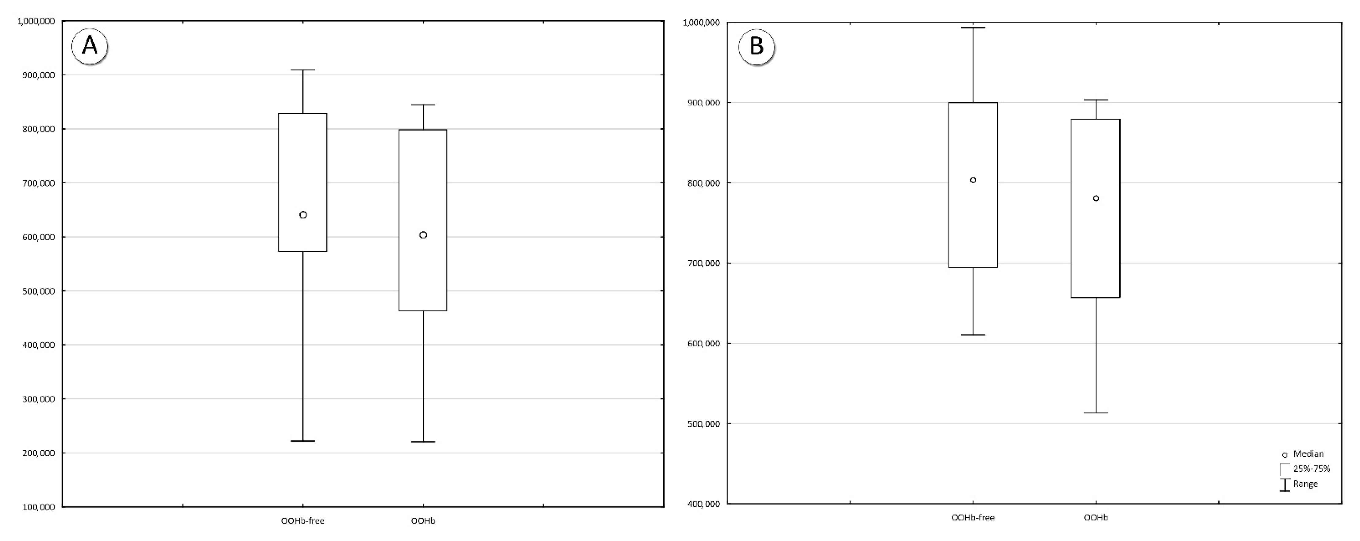
5.3. Two Scenario 3D Isovists Results

The 3D ISOVISTS was executed for each of 26 measurement points using two scenarios (“OOHb-free” and “OOHb”). Depending on the scenario variant, the changing proportions between VVV and OVV resulted in a statistically significant decrease of VVV in both case study areas to a similar extent (Figure 9). In both case studies, the VVV–OVV balance changes concern the vast majority (92.3%) of the measurement points; two points located at the measurement patches endings were identified with no change (

Table 2. The VVV–OVV balance results for “OOHB-free” and “OOHb scenarios”.

		OOHb-FREE				OOHb
No.	Measurement Point	VVV(m3)	OVV(m3)	VVV (%)	OVV (%)	VVV(m3)	OVV(m3)	VVV (%)	OVV (%)	VVV Change (%)
1	A1S1	606,578.13	493,421.88	55.1	44.9	606,578.13	493,421.88	55.1	44.9	0.00
2	A1S2	683,046.88	416,953.13	62.1	37.9	680,609.38	419,390.63	61.9	38.1	−0.22
3	A1S3	842,750.00	257,250.00	76.6	23.4	797,625.00	302,375.00	72.5	27.5	−4.10
4	A1S4	909,125.00	190,875.00	82.6	17.4	844,468.75	255,531.25	76.8	23.2	−5.88
5	A1S5	640,906.25	459,093.75	58.3	41.7	603,546.88	496,453.13	54.9	45.1	−3.40
6	A1S6	572,593.75	527,406.25	52.1	47.9	566,546.88	533,453.13	51.5	48.5	−0.55
7	A1L1	828,984.38	271,015.63	75.4	24.6	816,890.63	283,109.38	74.3	25.7	−1.10
8	A1L2	909,125.00	190,875.00	82.6	17.4	844,468.75	255,531.25	76.8	23.2	−5.88
9	A1L3	778,750.00	321,250.00	70.8	29.2	580,875.00	519,125.00	52.8	47.2	−17.99
10	A1L4	607,312.50	492,687.50	55.2	44.8	462,171.88	637,828.13	42.0	58.0	−13.19
11	A1L5	370,046.88	729,953.13	33.6	66.4	307,406.25	792,593.75	27.9	72.1	−5.69
12	A1L6	241,515.63	858,484.38	22.0	78.0	234,750.00	865,250.00	21.3	78.7	−0.62
13	A1L7	221,968.75	878,031.25	20.2	79.8	220,640.63	879,359.38	20.1	79.9	−0.12
14	A2S1	801,171.88	298,828.13	72.8	27.2	780,843.75	319,156.25	71.0	29.0	−1.85
15	A2S2	902,281.25	197,718.75	82.0	18.0	513,421.88	586,578.13	46.7	53.3	−35.35
16	A2S3	993,656.25	106,343.75	90.3	9.7	888,343.75	211,656.25	80.8	19.2	−9.57
17	A2S4	899,515.63	200,484.38	81.8	18.2	879,203.13	220,796.88	79.9	20.1	−1.85
18	A2S5	803,359.38	296,640.63	73.0	27.0	802,312.50	297,687.50	72.9	27.1	−0.10
19	A2S6	694,453.13	405,546.88	63.1	36.9	694,453.13	405,546.88	63.1	36.9	0.00
20	A2L1	641,031.25	458,968.75	58.3	41.7	640,734.38	459,265.63	58.2	41.8	−0.03
21	A2L2	887,593.75	212,406.25	80.7	19.3	884,234.38	215,765.63	80.4	19.6	−0.31
22	A2L3	909,234.38	190,765.63	82.7	17.3	903,625.00	196,375.00	82.1	17.9	−0.51
23	A2L4	826,671.88	273,328.13	75.2	24.8	812,359.38	287,640.63	73.9	26.1	−1.30
24	A2L5	759,843.75	340,156.25	69.1	30.9	737,265.63	362,734.38	67.0	33.0	−2.05
25	A2L6	669,312.50	430,687.50	60.8	39.2	657,390.63	442,609.38	59.8	40.2	−1.08
26	A2L7	610,640.63	489,359.38	55.5	44.5	605,906.25	494,093.75	55.1	44.9	−0.43

). The closer the distance between the observer (the measurement point) and the OOHb, the more significant VVV–OVV imbalance was noted. However, as emphasised in the discussion, distance is not the only explanatory variable of OVV increase.

5.3.1. The VVV–OVV Balance of Area “A”

The changes in VVV–OVV balance are described below using percentages and taking the “OOHb-free” scenario as a reference. In area “A”, the resulting changes range from 0.12% to 18%. The most significant change (18%) concerns the A1L3 measurement point, surrounded by 12 OOHb and distanced 6.2 m from the closest one (Figure 10). Furthermore, four OOHB visible from the A1L3 point were facing back; thus, the advertisement content was not visible from the analyzed point. This point out that the visual impact of OOHb infrastructure is not limited to its advertisement exposure area only. At the A1L3 measurement point, the OOHB infrastructure caused 197,845 m³ of OVV and the long-distance view-blocking effect. Specifically, the pedestrian observer loses the view of the green part of the Czechówka river valley, and they can see neither water nor bridge, the observer also loses the tenement house view at Niecała St. (tenement house built in 1914). The visual volume occlusion effect of the OOHb impacts the perceived landscape physiognomy too.

In area “A” center (points A1L2 and A1s4), the VVV decreases by 5.88% due to the viewing volume occlusion effect herein caused by 15 OOHb. The closest OOHb was 22.5 m distant, the farthest 104.8 m. Same as in the previously discussed point, four of the advertisements were facing back too. The above points out to the lack of spatial analytics in the spatial arrangements of the case study OOHb infrastructure and no references to landscape issues.

Averaging the results of area “A” measurement patches, it can be stated that the OOHb decreased the VVV by 25,937.5 m³ (2.36%) and by 70,071.4 m³ (6.37%) along “short” and “long” measurement patches. The same, the average volume of 291.9 m³ was obstructed on each meter of observer patch. The shorter path, along which OOHb formed a spot, results in a mean value of 129.7 m³ per one meter.

In general, the landscape openness of area A can be characterized as moderate (half-open) the mean VVV was 631746.4 m³ (57.4%). The OOHb scenario resulted in 52.9% and 47.1% of VVV and OVV proportions, respectively. On average, the OOHb reduces the OVV by 4.52%. Statistical significance of those changes has been confirmed by Wilcoxson and Sign test results (

Table 3. The area “A” VVV statistical significance test results along with basic statistic summary.

“A” Area	Mean	Median	Q1	Q3	Mini	Max	S.D.	Sign Test	Wilcoxon Test
OOHb-free	582,044.5	603,546.9	462,171.9	797,625.0	220,640.6	844,468.8	221,999.1	p = 0.001496	p = 0.002218
OOHb	631,746.4	640,906.3	572,593.8	828,984.4	221,968.8	909,125.0	233,638.4

).

The close range location of OOHb to a pedestrian path may have landscape quality consequences, but foremost it makes the advertisement ranged too closely hard to read. Furthermore, the advertising boards block the long-distance and city landmark view. The visual accessibility between observers’ locations influence the way in which the easy and the hard route is being determined, also landmarks obstruction contribute to wayfinding difficulty [53]. The OOHb are located mostly on the street intersections where the traffic slows down and the probability of advertising media content reaching increases. However, the street intersections are the place where pedestrians take a navigational decision where to head next, then limited views by the OOHb destroy this decision making process [54]. Therefore the OOHb view obstruction effect anticipates contributing to the pedestrian wayfinding issues. Summing up, area “A” points out some ill-conceived spatial configuration of the outdoor advertising media case study.

5.3.2. The VVV–OVV Balance of Area “B”

The spatial arrangements of OOHb differ in area “B”, specifically the multiple located OOHb in the N-W part, creating a high wall of advertisement billboards infrastructure. The wall height is up to 12.5 m (Figure 5). Furthermore, the OOHb spot arrangements make the VVV and OVV changes concern the measurement points located near the wall above rather than points gradually distanced from the OOHB spots. These specific arrangements also result in more meaningful changes concerning landscape physiognomy, composed among others by historic buildings of Lublins Caste (built-in XIII-XIV century) and Orthodox Church (built-in 1607–1633).

Foremost, area “B” is characterized by high landscape openness. The VVV were ranging from 993,656.25 m³ at the A2S3 to 610,640.625 m³ at the A2L7 measurement point. This openness makes this particular cityscape attractive to the OOHb industry investors, especially being not limited by the land-use zoning guidelines at this location. As a result of OOHb scenario calculations, the most significant visual impact was measured at the A2S2 point. The A2S2 point was located in front of the advertisement billboards wall, covering up to 90° of a 2D field of view. The 35.35% increase in OVV was noted, and the VVV was reduced from 902,281.25 to 513,421.875 m³.

Furthermore, the OOHB covered the views of Lublin Castle and Orthodox Church—an iconic historical landmark of Lublin City (Figure 11). The conflict with iconic landmarks points out the lack of consistency between the city’s outdoor advertising policy and land-use zoning. In fact, there is no outdoor advertising politics and faulty zoning. The 35% increase in OVV is regarded as a “red alert” for this particular location, not only because of the visual obstruction volume but foremost due to the historical content diminishing. The A2S3 was the second most affected by the OOHb occlusion effect measurement point. Its VVV decreased by 9.57% however, the Lublin Castle view was no longer blocked as the observer point was 57 m distant from the advertisement billboards wall. This yields some methodological recommendation not to referee the 3D isovist results to a single location only. Indeed, the adopted network of 13 measurement points does not expose the whole aspects of VP complexity in area “B”, however, it allows to point out the most problematic locations precisely and measure the impact on landscape openness. The averaged VVV–OVV balance of area “B” was 72.7% to 27.3%, respectively. The executed 3D isovist scenario has changed viewing volume proportions in favor of OVV up to 31.5% (the A2S2 point), on average, the VVV of area “B” was decreased by 4.2%. The same average OVV for “long” and “short” measurement patches was 0.82% and 8.12%, respectively. For each meter of the pedestrian observer patch, the value of 37.38 m³ and 446.54 m³ resulted in the “long” and “short” measurement patches. The significance of the changes above was confirmed by statistical tests (

Table 4. The area “B” VVV statistical significance test results along with basic statistic summary.

“B” Area	Mean	Median	Q1	Q3	Mini	Max	S.D.	Sign Test	Wilcoxon Test
OOHb-free	799,905.0	803,359.4	694,453.1	899,515.6	610,640.6	993,656.3	118,728.1	p = 0.001496	p = 0.002218
OOHb	753,853.4	780,843.8	657,390.6	879,203.1	513,421.9	903,625.0	124,274.8

).

Summing up, despite differences in spatial configuration between area “B” and “A”, the changes of averaged VVV value were similar, specifically 4.2% in area “A” and 4.52% in area “B”. This case study yields to the conclusion that OOHb infrastructure may reduce the averaged landscape openness by at least 4%. Considering the analyzed areas as a VP example, both are overwhelmed by outdoor advertisement. The averaged OVV increase is taken as the VP threshold, resulting in the total number of 6 and 2 points with the VP threshold exceeded in the “A” and “B” areas, respectively. In practice, VP diminishing activities should be focused on these specific points, this research method framework is an alternative strategy to the Clear City Law of San Paulo [55].

6. Discussion

This research takes voxels to measure the view volume changes describing the visual impact of specific outdoor advertisements infrastructure, the actor of the VP phenomenon. This study is attempts to quantify the VP using 3D isovist methods, to the best of the author knowledge, so far not undertaken as a research task in the scientific literature. The 3D isovist divides the observer’s view volume into visible (the VVV parameter) and not visible (the OVV parameter) subsets. Basically, the research is inspired by Alexander [56] architectural studies, who finds that outdoor open space has a positive impact on people’s well-being as well as Fry et al., [57] whose studies argue landscape openness as a key quality feature. Foremost, the research of Fisher–Gewirtzman has successfully captured the sense of openness in an architectural space [14,15,16]. From above, openness appears to be an essential landscape character for many European countries [58], for example, the Netherlands point the openness out as a core landscape quality [18]. This Polish case study results provide statistically significant evidence that OOHb impacts the visual properties of the viewsphere, precisely the visible and obstructed view volume, in disadvantage of landscape openness decrease.

The VVV decrease is a measure of visual impact, because the OVV is strongly related to the distance extended from viewpoint and billboard also its relative ratio can be discussed as a potentially suitable index describing the VP impact. Importantly, the discussed indicator could refer to every single OOHb, while the concept of VVV–OVV balance, proposed in this study, referees to human viewsphere [29]; here for technical reasons calculated with a 3D bounding box extent. The 3D indicator development is a good starting point for the author’s future research, but it should be emphasized that its applicability will be limited to the OOHb scenario only.

GIS scientists for policy-makers develop the described method, and urban planners end users. It aims to understand the impact of VP on cityscape qualities, herein explained using scientific methods. The proposed VVV and OVV parameters also extend the list of landscape visual character assessment indicators [59]. Above all, the research explains far-reaching changes in landscape visual structure due to outdoor advertisement spread—the billboardization [40]. I hope the research outcomes will enhance the fragile cityscape physiognomy understanding and contribute to landscape sustainability improvements [60]. The arguments presented in this work in references to, for example, the unhealthy impact of OOHb infrastructure LED illuminations [61] would raise the local authorities’ attention to the subject of VP.

Furthermore, the research was based on literature evidence concerning the influence of landscape openness [14,17,18] on the citizens subjective wellbeing [62]. Literature studies, however, refers more to buildings configuration and case study topography rather than advertisement billboards. Therefore, it is worth verifying the above statement against VP by, for example, using neuroscience-based methods [63]. For example, placing advertisements in very narrow public spaces would directly affect the enclosure by which extreme levels may block movement [9] and evoke claustrophobia [64]. This work does not analyze the personal ability to recognize enclosure which is, in fact, a consequence of natural selection [65], therefore this landscape study is focused on VVV–OVV balance. The proposed method relies on an accurate 3D city model, which according to the digital twin idea, can be published online, be walked around by the public for viewing the proposed development, and enable 3D research and experimentation too [66]. The most important variable, determining methodology replicability, is the availability of 3D geospatial data at high level of details. However, by using additional data on advertising exposure time and number of audiences, the method can be extended beyond the issue of VVV–OVV balance and used to optimize the OOHb localization in terms of advertisement benefit at minimum visual landscape impact.

Regardless of discussing VP consequences, it always refers to visual landscape resources; hence GIS-based visibility methods are expected at this end. The visibility model can explain the VP and the changes in the urban 3D morphology caused by OOHb, which is the case of this research. Typically, the object of qualitative landscape assessment is to provide the visibility range, size and percentage of the object in a full field of view [67]. Considering the relationship between landscape openness and landscape quality [17], this study emphasizes the geometric properties of visible volume subsets: the visible and occluded ones. The concept of view volume subsets extend the scope of the visual impact assessment analysis to date and points out that each new object added to the landscape would change physiognomy and openness.

Focusing on landscape quality issues and OOHb infrastructure management improvements can be achieved by using the VVV–OVV balance method to test various spatial configurations of OOHb. Specifically, the 3D isovist can verify if particular OOHb impacts the view corridors and iconic cityscape landmarks. Sophisticated 3D methods can support the view corridor protection policy [68], but they require local decision-makers involvement in 3D GIS technologies. The example of the Lublin case study reveals that still a lot could be done in this regard.

From a technical point of view, to solve the visibility, this study uses a 3D isovist. Usually, voxels and isovist are not enabled in off-the-shelf software and require code scripting or non-GIS software usage for example [69]. This limitation has been overcome here, as the ArcGIS Pro was used purposely to make the framework easy to replicate among GUI software users. The framework results from a well-thought-out compilation of tools, however, its limitations are discussed below.

A simplification is to expect a Boolean VP threshold, to say when the VP is and when it is not. VP, as with other visibility issues, has fuzzy characteristics [70]. Furthermore, the VP threshold will always be a matter of an individual case study. In other studies, the VP threshold was estimated using a proxy of public opinion and cumulative views [5]. This research uses the VVV–OVV balance, and its average changes did not exceed 4%. However, this raises the question about the impact of adopted bounding box size on resulting VVV–OVV parameters. The more extended the bounding box is, the more significant the values will be as a result. Thus, the different case study comparison requires either the use of unified bounding box size or an area quotient.

Furthermore, this research bounding box refers to literature recommendations and pre-test results. Alternatively, the 2D isovist analysis could be conducted first to find the maximum visibility radius [71], then use this radius as bounding box length and width extents. Additionally, a specific line of sight recommendation can be considered for cityscape 3D analyses [72], but always regarding variable computer processing power. Our research also found that the software used does not handle fine-scale voxels displaying, therefore 3D display properties should be verified too.

Paying attention to provide accurate results, the 3D symbol of high vegetation needs to be discussed too. Their geometry, herein adapted to the actual height of trees, is a generalization. Replacing 3D symbols with voxelized vegetation models [73] could make the results more accurate.

The last but not least limitation of the proposed method is the open space voxelization. Typically, spatial features like the trees, as mentioned earlier or buildings, are the object of voxelization. As input data, the 3D point cloud is being used, algorithms like octree-voxels are used to limit processed data. However, the challenge of future research is to develop a view volume voxelization algorithm, in fact, this is an empty space. Due to the lack of such GIS software algorithms, gridded voxels were used, which resulted in the extension of the analysis computation time.

7. Conclusions

Concluding, this research fills the knowledge gap in the VP related studies by providing the 3D visual impact assessment method of OOHb infrastructure referring to the landscape openness concept [14,56,57]. The study incorporates a commonly used 3D isovist method, however, it modifies the visible volume computation process with the line of sight and voxels, thus enabling small urban feature detection. The OOHb, located in line with pedestrian paths, can decrease the landscape openness up to 35%, the averaged level of visual impact achieved 4%, herein interpreted as case study VP threshold. The relationship between outdoor advertising and landscape openness has been explained using 3D GIS methods. The obtained results allow a better understanding of the visual landscape change caused by a vertical infrastructure, herein examined on the example of OOHb and in accordance with the author’s intention, will raise the awareness of the fragile nature of visual landscape.

References

1. Portella, A. Visual Pollution: Advertising, Signage and Environmental Quality; Ashgate Publishing: Farnham, UK, 2014. [Google Scholar]
2. Chmielewski, S. Chaos in motion: Measuring visual pollution with tangential view landscape metrics. Land 2020, 9, 515. [Google Scholar] [CrossRef]
3. Szczepańska, M.; Wilkaniec, A.; Škamlová, L. Visual pollution in natural and landscape protected areas: Case studies from Poland and Slovakia. Quaest. Geogr. 2019, 38, 133–149. [Google Scholar] [CrossRef] [Green Version]
4. Ahmed, N.; Islam, M.N.; Tuba, A.S.; Mahdy, M.R.C.; Sujauddin, M. Solving visual pollution with deep learning: A new nexus in environmental management. J. Environ. Manag. 2019, 248, 109253. [Google Scholar] [CrossRef] [PubMed]
5. Chmielewski, S.; Lee, D.; Tompalski, P.; Chmielewski, T.J.; Wężyk, P. Measuring visual pollution by outdoor advertisements in an urban street using intervisibility analysis and public surveys. Int. J. Geogr. Inf. Sci. 2016, 30, 801–818. [Google Scholar] [CrossRef]
6. Allahyari, H.; Salehi, E.; Zebardast, L. Evaluation of visual pollution in urban squares using SWOT, AHP, and QSPM techniques (Case study: Tehran squares of Enghelab and Vanak). J. Pollut. 2017, 3, 655–667. [Google Scholar]
7. Jana, M.K.; De, T. Visual pollution can have a deep degrading effect on urban and sub-urban community: A study in few places of Bengal, India, with special reference to unorganised billboards. Eur. Sci. J. 2015, 7881, 1–14. [Google Scholar]
8. Kamičaitytė-Virbašienė, J.; Godienė, G.; Kavoliūnas, G. Methodology of visual pollution assessment for natural landscapes. J. Sustain. Archit. Civ. Eng. 2016, 13, 80–91. [Google Scholar] [CrossRef] [Green Version]
9. Madleňák, R.; Hudák, M. Analysis of data needs and having for the integrated urban freight transport management system. Commun. Comput. Inf. Sci. 2016, 40, 135–148. [Google Scholar]
10. Śleszyński, P.; Kowalewski, A.; Markowski, T.; Legutko-Kobus, P.; Nowak, M. The contemporary economic costs of spatial chaos: Evidence from Poland. Land 2020, 9, 214. [Google Scholar] [CrossRef]
11. Hayward, S.C.; Franklin, S.S. Perceived openness-enclosure of architectural space. Environ. Behav. 1974, 6, 37. [Google Scholar]
12. Kaplan, R.; Kaplan, S. The Experience of Nature: A Psychological Perspective; Cambridge University Press: New York, NY, USA, 1989. [Google Scholar]
13. Coeterier, J.F. Cues for the perception of the size of space in landscapes. J. Environ. Manag. 1994, 42, 333–347. [Google Scholar] [CrossRef]
14. Fisher-Gewirtzman, D.; Burt, M.; Tzamir, Y. A 3-D visual method for comparative evaluation of dense built-up environments. Environ. Plan. B Plan. Des. 2003, 30, 575–587. [Google Scholar] [CrossRef] [Green Version]
15. Shach-Pinsly, D.; Fisher-Gewirtzman, D.; Burt, M. Visual exposure and visual openness: An integrated approach and comparative evaluation. J. Urban Des. 2011, 16, 233–256. [Google Scholar] [CrossRef]
16. Fisher-Gewirtzman, D. The association between perceived density in minimum apartments and spatial openness index three-dimensional visual analysis. Environ. Plan. B Urban Anal. City Sci. 2017, 44, 764–795. [Google Scholar] [CrossRef]
17. Weitkamp, G. Mapping landscape openness with isovists. Res. Urban. Ser. 2011, 2, 205–223. [Google Scholar]
18. Weitkamp, G.; Bregt, A.; van Ron, L. Measuring visible space to assess landscape openness. Landsc. Res. 2011, 36, 127–150. [Google Scholar] [CrossRef]
19. Stamps, A.E., III; Smith, S. Environmental enclosure in urban settings. Environ. Behav. 2002, 34, 781–794. [Google Scholar] [CrossRef]
20. Shi, S.; Gou, Z.; Chen, L.H.C. How does enclosure influence environmental preferences? A cognitive study on urban public open spaces in Hong Kong. Sustain. Cities Soc. 2014, 13, 148–156. [Google Scholar] [CrossRef]
21. Kamicaityte-Virbasiene, J.; Samuchovi, O. Free standing billboards in a road landscape: Their Visual impact and its regulation possibilities (Lithuanian case) Júrate Kamicaityté-Virbasiené, Ona Samuchoviené. Environ. Res. Eng. Manag. 2013, 4, 66–78. [Google Scholar]
22. Chmielewski, S.; Lee, D. Gis-based 3D visibility modelling of outdoor advertising in urban areas. In Proceedings of the XV SGEM Conference Proceedings, Albena, Bulgaria, 18–24 June 2015; pp. 923–930. [Google Scholar] [CrossRef]
23. Benedikt, M.L. To take hold of space: Isovists and isovist fields. Env. Plan B Plan Des. 1979, 6, 47–65. [Google Scholar] [CrossRef]
24. Felleman, J.P. Landscape Visibility Mapping: Theory and Practice School of Landscape Architecture; State University of New York, College of Environmental Forestry: Syracuse, NY, USA, 1979. [Google Scholar]
25. Batty, M. Exploring isovist fields: Space and shape in architectural and urban morphology. Environ. Plan. B Plan. Des. 2001, 28, 123–150. [Google Scholar] [CrossRef] [Green Version]
26. Hernández, J.; García, L.; Ayuga, F. Integration methodologies for visual impact assessment of rural buildings by geographic information systems. Biosyst. Eng. 2004, 88, 255–263. [Google Scholar] [CrossRef]
27. Sahraoui, Y.; Vuidel, G.; Joly, D.; Foltête, J.C. Integrated GIS software for computing landscape visibility metrics. Trans. GIS 2018, 22, 1310–1323. [Google Scholar] [CrossRef]
28. Chmielewski, S.; Tompalski, P. Estimating outdoor advertising media visibility with voxel-based approach. Appl. Geogr. 2017, 87, 1–13. [Google Scholar] [CrossRef]
29. Yang, P.P.J.; Putra, S.Y.; Li, W. Viewsphere: A GIS-based 3D visibility analysis for urban design evaluation. Environ. Plan. B Plan. Des. 2007, 34, 971–992. [Google Scholar] [CrossRef] [Green Version]
30. Jiang, Z.; You, W.; Ding, W. Calculation of ground view factor as an index for urban thermal environment optimization. Energy Procedia 2017, 142, 2996–3001. [Google Scholar] [CrossRef]
31. Dirksen, M.; Ronda, R.J.; Theeuwes, N.E.; Pagani, G.A. Sky view factor calculations and its application in urban heat island studies. Urban Clim. 2019, 30, 100498. [Google Scholar] [CrossRef]
32. Bernard, J.; Bocher, E.; Petit, G.; Palominos, S. Sky view factor calculation in urban context: Computational performance and accuracy analysis of two open and free GIS Tools. Climate 2018, 6, 60. [Google Scholar] [CrossRef] [Green Version]
33. Gong, F.Y.; Zeng, Z.C.; Zhang, F.; Li, X.; Ng, E.; Norford, L.K. Mapping sky, tree, and building view factors of street canyons in a high-density urban environment. Build Environ. 2018, 134, 155–167. [Google Scholar] [CrossRef]
34. Bosselmann, P. Representation of Places: Reality and Realism in City Design; University of California Press: Berkeley, CA, USA, 1998. [Google Scholar]
35. Morello, E.; Ratti, C. A digital image of the city: 3D isovists in Lynchs urban analysis. Environ. Plan. B Plan. Des. 2009, 36, 837–853. [Google Scholar] [CrossRef] [Green Version]
36. Lin, T.; Lin, H.; Hu, M. Three-dimensional visibility analysis and visual quality computation for urban open spaces aided by Google SketchUp and Web GIS. Environ. Plan. B Urban Anal. City Sci. 2015, 44, 618–646. [Google Scholar] [CrossRef]
37. Tara, A.; Beleski, P.; Ninsalam, Y. Towards managing visual impacts on public spaces: A quantitative approach to study visual complexity and enclosure using visual bowl and fractal dimension in 3D. J. Digit. Landsc. Archit. 2019, 4, 21–32. [Google Scholar]
38. Park, C.; Ha, J.; Lee, S. Association between three-dimensional built environment and urban air temperature: Seasonal and temporal differences. Sustainability 2017, 9, 1338. [Google Scholar] [CrossRef] [Green Version]
39. Tara, A.; Lawson, G.; Renata, A. Measuring magnitude of change by high-rise buildings in visual amenity conflicts in Brisbane. Landsc. Urban Plan. 2021, 205, 103930. [Google Scholar] [CrossRef]
40. Gomez, J.E.A. The billboardization of Metro Manila. Int. J. Urban Reg. Res. 2013, 37, 186–214. [Google Scholar] [CrossRef]
41. Karami, S.; Taleai, M. An innovative three-dimensional approach for visibility assessment of highway signs based on the simulation of traffic flow. J. Spat. Sci. 2020, 1–15. [Google Scholar] [CrossRef]
42. Elena, E.; Cristian, M.; Suzana, P. Visual pollution: A new axiological dimension of marketing? Ann. Fac. Econ. 2012, 1, 820–826. [Google Scholar]
43. Enache, E.; Morozan, C.; Purice, S. Visual pollution: A new axiological dimension of marketing. In Proceedings of the 8th Edition of the International Conference “European Integration—New Challenges” EINCO2012, Oradea, Romania, 25–26 May 2012; pp. 2046–2051. Available online: http://anale.steconomiceuoradea.ro/volume/2012/proceedings-einco-2012.pdf (accessed on 5 May 2021).
44. Hamilton, J.L.; Gerald, J. Visual Pollution Study, a Report to the Citizens of Jacksonville; Jacksonville Community Council, Inc.: Jacksonville, FL, USA, 1985; Available online: https://digitalcommons.unf.edu/jcci/4 (accessed on 5 May 2021).
45. Polish National Geoportal. Available online: www.geoportal.gov.pl (accessed on 10 August 2020).
46. American Society of Photogrammetry and Remote Sensing. Lidar LAS Specification, Version 1.2. 2008. Available online: https://www.asprs.org/divisions-committees/lidar-division/laser-las-file-format-exchange-activities (accessed on 10 March 2021).
47. Barnes, C.; Balzter, H.; Barrett, K.; Eddy, J.; Milner, S.; Suárez, J.C. Individual tree crown delineation from airborne laser scanning for diseased larch forest stands. Remote Sens. 2017, 9, 231. [Google Scholar] [CrossRef] [Green Version]
48. Hounsfield, G.N. Computed medical imaging. J. Comput. Assist. Tomogr. 1980, 4, 665–674. [Google Scholar] [CrossRef] [PubMed]
49. Bremer, M.; Mayr, A.; Wichmann, V.; Schmidtner, K.; Rutzinger, M. A new multi-scale 3D-GIS-approach for the assessment and dissemination of solar income of digital city models. Comput. Environ. Urban Syst. 2016, 57, 144–154. [Google Scholar] [CrossRef]
50. Pyysalo, U.; Oksanen, J.; Sarjakoski, T. Viewshed analysis and visualisation of landscape voxel models. In Proceedings of the 24th International Cartography Conference, Santiago, Chile, 15–21 November 2009. [Google Scholar]
51. Palmer, J.F. The contribution of a GIS-based landscape assessment model to a scientifically rigorous approach to visual impact assessment. Landsc. Urban Plan. 2019, 189, 80–90. [Google Scholar] [CrossRef]
52. Starek, M.J.; Chu, T.; Mitasova, H.; Harmon, R.S. Viewshed simulation and optimisation for digital terrain modelling with terrestrial laser scanning. Int. J. Remote Sens. 2020, 41, 6409–6426. [Google Scholar] [CrossRef]
53. Natapov, A.; Kuliga, S.; Dalton, R.C.; Hölscher, C.H. Linking building-circulation typology and wayfinding: Design, spatial analysis, and anticipated wayfinding difficulty of circulation types. Archit. Sci. Rev. 2020, 63, 34–46. [Google Scholar] [CrossRef]
54. Natapov, A.; Fisher-Gewirtzman, D. Visibility of urban activities and pedestrian routes: An experiment in a virtual environment. Comput. Environ. Urban Syst. 2016, 58, 60–70. [Google Scholar] [CrossRef]
55. Drigo, M.O. Cidade/Invisibilidade e Cidade/Estranhamento: São Paulo Antes e Depois da lei “Cidade Limpa”. Galáxia 2009, 17, 49–64. Available online: https://revistas.pucsp.br/galaxia/article/view/2097 (accessed on 11 May 2021).
56. Alexander, C.A. Pattern Language: Towns, Buildings, Construction; Oxford University Press: Oxford, UK, 1977; Available online: https://arl.human.cornell.edu/linked%20docs/Alexander_A_Pattern_Language.pdf (accessed on 20 March 2021).
57. Fry, G.; Tveit, M.S.; Ode, Å.; Velarde, M.D. The ecology of visual landscapes: Exploring the conceptual common ground of visual and ecological landscape indicators. Ecol. Indic. 2009, 9, 933–947. [Google Scholar] [CrossRef]
58. Wascher, D. European Landscape Character Areas: Typologies, Cartography and Indicators for the Assessment of Sustainable Landscapes. Final Project Report as Deliverable from the E.U.’s Accompanying Measure Project European Landscape Character Assessment Initiative (ELCAI); Landscape Europe: Wageningen, The Netherlands, 2005. [Google Scholar]
59. Tveit, M.; Ode, Å.; Fry, G. Key concepts in a framework for analysing visual landscape character. Landsc. Res. 2007, 31, 229–255. [Google Scholar] [CrossRef]
60. Selman, P. What do we mean by sustainable landscape? Sustain. Sci. Pract. Policy 2008, 4, 23–28. [Google Scholar] [CrossRef]
61. Zielinska-Dabkowska, K.M. Make lighting healthier. Nature 2018, 553, 274–276. [Google Scholar] [CrossRef] [PubMed]
62. Jayawickreme, E.; Forgeard, M.J.C.; Seligman, M.E.P. The engine of well-being. Rev. Gen. Psychol. 2012, 16, 327–342. [Google Scholar] [CrossRef]
63. Olszewska-Guizzo, A. Neuroscience-based urban design for mentally-healthy cities. In Urban Health and Wellbeing Programme Policy Briefs; Springer Nature: Basingstoke, UK, 2021; Volume 2, pp. 13–16. [Google Scholar] [CrossRef]
64. Alkhresheh, M. Enclosure as a Function of Height-To-Width Ratio and Scale: Its Influence on Users Sense of Comfort and Safety in Urban Street Space. Ph.D. Thesis, University of Florida, Gainesville, FL, USA, 2007. [Google Scholar]
65. Stamps, A.E. Evaluating enclosure in urban sites. Landsc. Urban Plan. 2001, 57, 25–42. [Google Scholar] [CrossRef]
66. White, G.; Zink, A.; Codecá, L.; Clarke, S. A digital twin smart city for citizen feedback. Cities 2021, 110, 103064. [Google Scholar] [CrossRef]
67. Wrózyński, R.; Sojka, M.; Pyszny, K. The application of GIS and 3D graphic software to visual impact assessment of wind turbines. Renew. Energy 2016, 96, 625–635. [Google Scholar] [CrossRef]
68. London View Management Framework SPG, Mayor of London. March 2012. Available online: https://www.london.gov.uk/what-we-do/planning/implementing-london-plan/london-plan-guidance-and-spgs/london-view-management (accessed on 8 January 2021).
69. Suleiman, W.; Joliveau, T.; Favier, E. A New Algorithm for 3D Isovists. In Advances in Spatial Data Handling; Timpf, S., Laube, P., Eds.; Springer: Berlin/Heidelberg, Germany, 2013; pp. 157–173. [Google Scholar] [CrossRef]
70. Fisher, P.F. Probable and fuzzy models of the viewshed operation. In Innovations in GIS; Worboys, M., Ed.; Taylor & Francis: London, UK, 1984; pp. 161–175. [Google Scholar]
71. Heinrich, C.H.; Candela, P. BRISK: Binary Robust Invariant Scalable Keypoints. In Proceedings of the 13th International Conference on Computer Vision, Barcelona, Spain, 6–13 November 2011; pp. 2548–2555. Available online: www.research-collection.ethz.ch/handle/20.500.11850/43288 (accessed on 20 May 2021).
72. Mor, M.; Fisher-Gewirtzman, D.; Yosifof, R.; Dalyot, S. 3D visibility analysis for evaluating the attractiveness of tourism routes computed from social media photos. ISPRS Int. J. Geo-Inf. 2021, 10, 275. [Google Scholar] [CrossRef]
73. Phattaralerphong, J.; Sinoquet, H. A method for 3D reconstruction of tree crown volume from photographs: Assessment with 3D-digitized plants. Tree Physiol. 2005, 25, 1229–1242. [Google Scholar] [CrossRef] [PubMed] [Green Version]
Figure 1. Two subsets of observer’s view volume: the visible view volume (VVV) referred to landscape openness (blue) and occluded view volume (OVV, red color). The subsets are represented using voxels, the voxels visibility status is determined by 3D ISOVIST analysis. The OOHb infrastructure is orange. The subsets balance is analyzed within the voxels bounding box, centered to the observer’s position (the cross-section view).
Ijgi 10 00656 g001
Figure 2. The out of home advertising media location in Lublin City, Poland: the insight into VP spatial extent (own elaboration based on field measurement campaign in 2015).
Ijgi 10 00656 g002
Figure 3. The case study areas and measurement points located along with pedestrian patches: (A) the area “A”, (B) the area “B”, distanced 1 km from each other.
Ijgi 10 00656 g003
Figure 4. The method workflow steps: (1) a case study 3D city model creation through open geospatial data integration in 3D-GIS software; (2) filling the empty space remaining in the 3D model with voxels; (3) the voxel visibility determination using 3D Isovist calculated in OOHb-free and OOHb scenario; (4) the visible view volume change detection and statistical significance test.
Ijgi 10 00656 g004
Figure 5. The profile view of a 3D point cloud representing the actual dimension of OOHb infrastructure (A) and high-resolution DSM of OOHb infrastructure (B).
Ijgi 10 00656 g005
Figure 6. The spatial extent of the 3D ISOVISTS analysis in areas “A” (A) and “B” (B). The moving bounding box from one measurement point to the next (spaced 40 m) results in a bounding box overlay effect; the overlay border is an extent of the analysis.
Ijgi 10 00656 g006
Figure 7. The visualization of the 3D city model (area B example). The red and purple dots are the measurement points, the OOHb infrastructure is presented as orange 3D symbols.
Ijgi 10 00656 g007
Figure 8. The effect of voxel sizes on the VVV (blue) and OVV (red) measurement accuracy: (A) 10 m voxels, (B) 5 m voxels, (C) 2.5 m voxels, (D) 1.25 m voxels. The voxel size has been thinned by 0.1 m to highlight the edges.
Ijgi 10 00656 g008
Figure 9. The visible volume decreases (the VVV parameter) as a result of OOHb occurrence in the landscape in botch cases studies: (A) the area “A”, (B) the area “B”.
Ijgi 10 00656 g009
Figure 10. The view volume subsets of area “A” in the OOHb scenario: the VVV (blue) and extensive red volume of obstructed view; the Czechówka river valley view is fully covered from A1L3 observer position.
Ijgi 10 00656 g010
Figure 11. The view occlusion extremum (red) at A2S2 measurement point. From this observer location, the OOHb crate the infrastructure wall decreasing perceived landscape openness and blocking the city landmarks views (the Lublin Castle and the Old Town in the background).
Ijgi 10 00656 g011