A Novel Ultra-Wideband Double Difference Indoor Positioning Method with Additional Baseline Constraint

Abstract

Ultra-wideband (UWB) technology is suitable for indoor positioning owing to its high resolution and penetration. However, the current UWB positioning methods not only fail to fully analyze errors, but do not have the ability to eliminate gross and large random errors. In this article, the errors of UWB indoor positioning are analyzed comprehensively, and the basic function model is given. An indoor positioning method based on a double difference UWB with ranging observations is proposed and realized. In the proposed method, two UWB rover stations and a common base station are introduced, and the known baseline length between two rovers is used as the constraint condition for quality control. The observations and coordinate estimations are constrained by the prior and posteriori, respectively, and the weight of ranging observations with large residuals is reduced. Two groups of static experiments are designed. After adopting the proposed method, the plane error of one rover is 3.4 cm and 2.1 cm, and plane error of another rover is 3.3 cm and 2.0 cm, respectively. The positioning precision is improved by more than 80% compared with the traditional method. In the dynamic experiment, the coordinates of the starting and ending point obtained by the proposed method are basically consistent with the truth value, and the positioning results are close to the reference trajectory. The experimental results show that the proposed method can eliminate systematic and large random errors and improve the positioning precision effectively.

1. Introduction

Nowadays, global satellite navigation systems (GNSS) are widely used for outdoor positioning and navigation and verified in many high-precision positioning fields. Common GNSS high-precision positioning technologies include real-time kinematic (RTK) and precise point positioning (PPP). They are the representatives of outdoor dynamic high-precision positioning solutions and, nowadays, are fully realized. However, GNSS signal is unreliable in GNSS-denied conditions due to occlusion, such as in indoor environments [1]. Therefore, a variety of indoor positioning technologies are gradually researched. For example, indoor positioning technologies with an accuracy of 3–5 m, such as Wi-Fi, Bluetooth, ZigBee and geomagnetism, can be used in emergency security, intelligent warehousing, precision marketing and mobile health. While audio, UWB, pseudolite and infrared positioning technologies with high-precision positioning accuracy are commonly used in aircraft manufacturing, large facilities monitoring, mine or tunnel engineering geodesy and robot intelligent positioning navigation. Among them, UWB technology is considered to be suitable for high-precision indoor positioning because of its advantages of fast transmission, strong penetration and anti-multipath fading ability [2].

The research into navigation and positioning generally focuses on the anchors arrangement, positioning algorithm and data fusion, error analysis and quality control. Similarly, most of the research on UWB indoor positioning focuses on the anchors arrangement, positioning algorithm, error modeling including non-line of sight (NLOS) and noise.

With regard to the anchors arrangement, the geometric dilution of precision (GDOP), Cramer–Rao lower bound (CRLB) and Root mean square error (RMSE) are usually used as objective functions. Especially the RMSE and GDOP are widely utilized as metrics to evaluate the optimal anchors arrangement [3]. Lin et al. [4] used a multi-lateration method to deal with the anchors arrangement problem, and the minimal position dilution of precision (PDOP) was the goal of optimization. Monica et al. [5] proposed an approach of the optimized placement of anchor nodes using the criterion of minimizing the average RMSE. Chen et al. [6] used the genetic algorithm (GA) to optimize locations of the anchor nodes, and the optimization objective was to minimize the average RMSE. Based on the Chan algorithm, Li et al. [7] analyzed the base station arrangement method in combination with the system construction site. Their optimization objective function was similar to that in the previous literature. Pan et al. [8] considered CRLB and coverage degree criterion as the objective function of the differential evolution (DE) algorithm, simultaneously. Wang et al. [9] proposed a search method for the optimal arrangement of the reference nodes based on a genetic algorithm. Wang et al. [10] proved that the dilution of precision DOP could not be used as the decisive metric for the configuration and optimization of the anchors. In fact, it was difficult to find a ubiquitous arrangement optimization principle due to the multipath and NLOS problems in the indoor environment. The anchors arrangement can only be adjusted according to the actual situation.

In terms of a UWB positioning algorithm, the Chan algorithm and nonlinear least squares estimation are often used for positioning the calculation if no extra nodes are used [2]. Some errors can also be corrected in advance or estimated according to the environment-related parameters [11]. These solutions are widely developed and discussed. In order to expand the availability of positioning, other positioning technologies are integrated with UWB technology. Geng et al. [12] fused UWB and ZigBee technologies using maximum likelihood estimation. Graichen et al. [13] applied occupancy grid maps (OGMs) to assist UWB positioning, and the proposed method increased the positioning accuracy. Krapež et al. [14] adopted additional calibration modules (CMs) in a 3D UWB positioning system. The results showed that the calibration before positioning could effectively improve the positioning accuracy. Wang et al. [15] proposed several positioning algorithms for different indoor scenes. The improved UWB location algorithm could meet a variety of positioning requirements. The most common method was to integrate UWB with inertial navigation system (INS). Li et al. [16] introduced map matching to optimize PPP/INS/UWB tight coupling positioning, which could effectively improve the positioning accuracy. Nguyen et al. [17] fused the inertial measurement unit (IMU) and UWB with camera. UWB ranging observations were focused on and the elimination of time offset was studied. The experimental results were clearly better than the traditional methods. In addition, Li et al. [18] proposed applying a particle filter to IMU/UWB positioning. Li et al. [19] used an extended Kalman filter (EKF) to improve the positioning accuracy of UWB and adopted an error-state Kalman filter (ESKF) to fuse UWB and IMU. Guo et al. [20] realized an indoor positioning method based on pedestrian dead reckoning (PDR) and UWB. The average error could reach up to a decimeter. Wang et al. [21] proposed a zero-velocity update (ZUPT)/UWB fusion algorithm based on graph optimization, with an accuracy of 0.4 m. The same idea was also presented by Zhang et al. [22]. Lutz et al. [23] proposed to combine UWB and a visual–inertial navigation system (VINS) to provide accurate pose estimations. Additionally, the drift in VINS could be alleviated. Actually, INS/UWB integration could improve positioning accuracy and availability, and maintain the continuity of positioning results when the UWB signal was missing. However, INS could not be calibrated when the UWB positioning accuracy was not guaranteed. Therefore, the error analysis and quality control of the UWB positioning results was very crucial.

Many studies focused on positioning error analysis and quality control. Bharadwaj et al. [24] studied the effect of human position on line-of-sight (LOS) and NLOS observations of UWB. Cao et al. [25] calibrated the UWB in the LOS scene and used three estimation methods to improve the positioning accuracy in the NLOS scene. Yang et al. [26] introduced the concepts of “virtual inertial point” and “environmental factor” to compensate the NLOS error in UWB indoor positioning. Zhang et al. [27] proposed a phase-difference-of-arrival (PDOA)-assisted UWB positioning method for the NLOS environment. In addition, neural networks were used to classify and recognize LOS/NLOS signals [28,29,30,31]. For example, Cui et al. [32] proposed a LOS/NLOS identification method based on a Morlet wave transform and convolutional neural networks. As for the processing of UWB error (including NLOS), a robust and adaptive Kalman filter was often utilized [33,34,35]. In addition, Xia et al. [36] applied a particle swarm optimization (PSO) algorithm for UWB positioning. The traditional PSO algorithm was used to obtain the initial value, and all the ranging information was applied to refine the positioning result, which effectively reduced the ranging error. However, the signal error was not classified, and for the analyses in these methods, the quality was not been controlled either. In fact, the analysis of UWB positioning errors was of great significance to understand its essence.

In addition to the theoretical research, UWB is widely used for the real-time high-precision positioning in indoor industrial engineering. For example, the status of people and equipment in coal operation are available at any time in the UWB mine personnel positioning system. Early warning and rescue measures can be provided. Furthermore, UWB technology is commercially applied to high-precision indoor and outdoor cable channel inspection. The Local Sense UWB precise positioning system developed by Tsinghua University has a positioning accuracy of 10 cm [2]. It solved the problem of the inability to precisely position components, equipment, vehicles and personnel in the industrial field, such as electric power, tunnels, and in the coal and chemical industry. The UWB system developed by Zebra Company of the United States achieved a sub-meter positioning precision and hwas applied in warehousing and logistics [37]. Ubisense Company in the UK launched the UWB-based transmitting and receiving module. The system measures the arrival time difference and the angle of arrival of the signal, and obtains the three-dimensional coordinates of the target according to the positioning algorithm. The error of the three-dimensional coordinates can be controlled within 15 cm with the Ubisense system [37]. DW1000, launched by the Decawave (now Qorvo) company, is a widely used UWB product [38] which is applied to many UWB-integrated development companies and scientific research institutions in colleges and universities. Wen et al. [39] also put forward a new strategy combining the downlink time difference of arrival (TDOA) based on real-time UWB in tunnels and highway scenarios. While the accuracy only reached 1 decimeter to 1 m. Hasan et al. [40] used UWB to compensate the position of automated guided vehicles (AGV) for the distribution of goods, scheduling of machine processes and coordination. Lawrence et al. [41] proposed using three UWB tags to determine the positions and attitudes of the mobile laser scanner for building information modeling (BIM) 3D data collection.

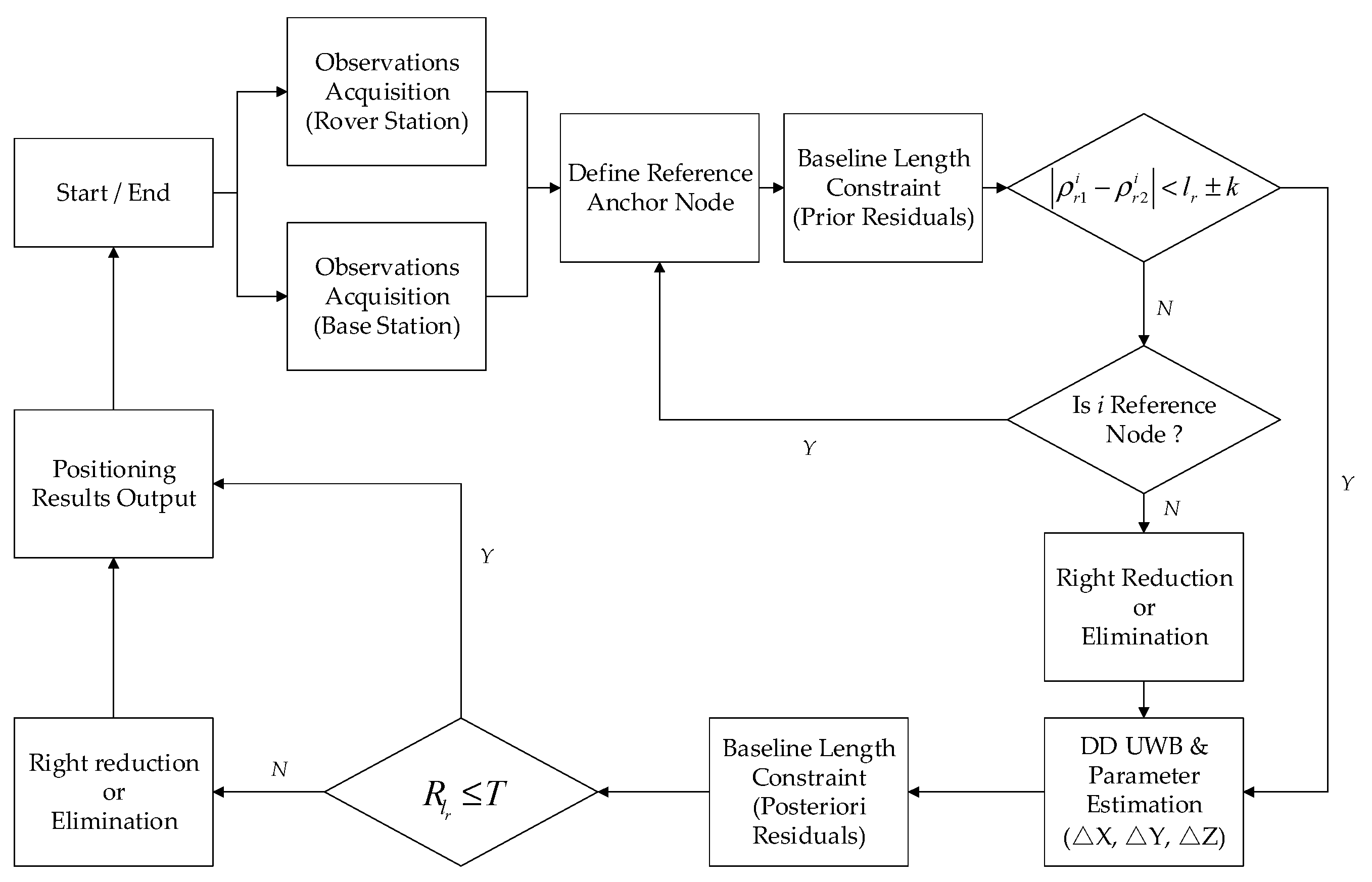
Although UWB positioning systems in industrial engineering are widely applied, there are still many details that can be further optimized, especially in precision, error analysis and quality control. Current research tends to focus on either error modelling and correction, or error elimination using a robust method. However, it is essential to classify errors to find main factors affecting the positioning. In this article, the main error that affects the accuracy is obtained through the exploration of UWB errors. Combined with the actual ranging observations, it is verified that the ranging errors are mainly composed of systematic and random errors. Regarding GNSS double difference technology, time-independent error components in UWB ranging observations are processed by a differential method, and a positioning algorithm based on double difference (DD) UWB ranging observations is proposed and deduced. Then, we introduce two rover stations to form a known baseline, which is used as an additional condition to constrain the original observations and coordinate the estimation values from the perspective of prior and posteriori. Therefore, the weight of ranging observations with large residual errors is reduced. Finally, through the experiments, the proposed method is verified to eliminate the systematic errors and large random errors effectively. The proposed method has the ability to control the quality of positioning the results and guarantees a precision at the centimeter level. For the convenience of description, the proposed method is named BC-DUWB (baseline constrained double difference UWB positioning).

2. Methodology

2.1. UWB Ranging

2.1.1. Two-Way Time of Flight Ranging

The UWB devices used in this article are PulsON410 and 440 (hereinafter referred to as P410 and P440) manufactured by Time Domain Company. Range observations between the anchor node and the tag are obtained using the Two-Way Time of Flight (TW-TOF) ranging approach. Firstly, a positioning tag send a request to an anchor node. Then, the anchor node returns a response to the positioning tag after an observation is obtained. Finally, the tag takes an observation, incorporates the tag observation and a range observation is calculated after the tag receives the response. When combined, the speed of light, time to send the request, time to return the response, time to receive the response, and the centimeter-level distance observation can be calculated. TW-TOF ranging method does not require time synchronization between anchor nodes. The schematic diagram of TW-TOF is shown in Figure 1.

The distance P between the anchor node and positioning tag can be expressed by the following formula:

$$P=c\times \left[\left(Ta2-Ta1\right)-\left(Tb2-Tb1\right)\right]/2$$

(1)

where c is the speed of light; Ta1 is the time that the anchor node sends the request to the positioning tag; Ta2 is the time that the anchor node receives the response from the positioning tag; Tb1 is the time that the positioning tag receives the request from the anchor node; and Tb2 is the time that the positioning tag sends the request to the anchor node.

2.1.2. Error Analysis of UWB Ranging

Although the clock drift error is not considered in the TW-TOF ranging method, many errors in UWB ranging derive from a lack of discussion. In this article, UWB ranging errors are classified into the following three categories in

Table 1. Errors of UWB Indoor Positioning.

Category	Errors
Anchor-Nodes Related	Antenna phase center deviation, electrical delay, known coordinate error
Tags Related	Antenna phase center deviation, electrical delay, noise
Propagation-path Related	Multipath, NLOS propagation error, electromagnetic interference

and analyzed comprehensively.

The phase-center deviation is caused by the non-coincidence of the geometric center and the phase center, which vary with the intensity and direction of the signal. Actually, there is an electrical delay between the antenna surface and internal sampler of the electronical device. Additionally, each device used in this paper is pre-programmed with an internal estimate to represent the electrical delay. The electrical delay is time-independent and only related to electronic devices and antenna types. It is also defined as the antenna delay in some articles [23]. The base station coordinate error is small, since the base station coordinate is generally obtained by other high-precision measurement technologies. In this article, a total station is used for the base station coordinate measurement. Total station is an optical instrument commonly used in construction, surveying and civil engineering. The measurement accuracy can reach mm level. For ease of understanding, the coordinate error of the base station is analogous to the orbit error in GNSS. Multipath and NLOS propagation errors are two difficult problems to be solved in positioning, especially in the complex indoor environment. UWB has a strong penetration ability in most cases, and the penetration error is related to the thickness of obstacles, such as wood and walls. In this article, the penetration error is regarded as NLOS error. Furthermore, irrelevant radio equipment should be placed away from anchor nodes and positioning stations during the measurement to avoid the electromagnetic interference.

2.2. The Proposed UWB Positioning Method

2.2.1. UWB Positioning Principle

According to the summary of UWB ranging errors, the ranging observations of UWB devices can be expressed by the following function model, which is proposed by referring to the GNSS error model [42]:

$$P_{rk}^s={\rho }_{rk}^s+e_r+e_s+A_r+A^s+\delta {\rho }_{rk}^s+{\epsilon }_{rk}^s+m_{rk}^s$$

(2)

where k is the current epoch, r is the UWB positioning tag, and s is the UWB anchor node; $P_{rk}^s$ represents UWB ranging observations; ${\rho }_{rk}^s$ represents the truth value of geometric distance between the UWB anchor node and the positioning tag; $e_r$ represents the electronic delay of UWB tags; $e_s$ is the electronic delay of UWB anchor nodes; A_r and A^s represent the antenna phase center deviation of tags and anchor nodes, respectively; $\delta {\rho }_{rk}^s$ is the equivalent distance error caused by inaccurate anchor nodes coordinates; ${\epsilon }_{rk}^s$ is noise while $m_{rk}^s$ represents multipath and NLOS signals. Among them, noise, multipath and anchor node coordinate deviation may not be the same at different epochs. The truth value of geometric distance can be expressed as:

$${\rho }_{rk}^s=\sqrt{{(x^s-x_{rk})}^2+{(y^s-y_{rk})}^2+{(z^s-z_{rk})}^2}$$

(3)

where $(x^s,y^s,z^s)$ are the coordinates of anchor nodes and $(x_{rk},y_{rk},z_{rk})$ are the coordinates of tags to be estimated.

If errors in Formula (2) are all regarded as random errors, there are only three unknown parameters: x_rk, y_rk, and z_rk.

When ranging observations of the tag to n (n > 3) anchor nodes are measured synchronously, assuming ${\rho }^{\prime }{}_{rk}^s$ is a ranging observation at k epoch without considering the random error, the equations are as follows:

$$\begin{array}{c}{\rho }^{\prime }{}_{rk}^1=\sqrt{{(x^1-x_{rk})}^2+{(y^1-y_{rk})}^2+{(z^1-z_{rk})}^2}\\ ⋮\\ {\rho }^{\prime }{}_{rk}^n=\sqrt{{(x^n-x_{rk})}^2+{(y^n-y_{rk})}^2+{(z^n-z_{rk})}^2}\end{array}$$

(4)

where s = 1, 2, …, n.

Regarding $(x_{r0},y_{r0},z_{r0})$ as the approximate coordinates of the tag, ranging observations are differentiated and linearized:

$$\delta {\rho }_{rk}^s=\frac{x_{r0}-x^s}{{\rho }_{r0}^s}\cdot \delta x_{rk}+\frac{y_{r0}-y^s}{{\rho }_{r0}^s}\cdot \delta y_{rk}+\frac{z_{r0}-z^s}{{\rho }_{r0}^s}\cdot \delta z_{rk}$$

(5)

where:

$${\rho }_{r0}^s=\sqrt{{(x^s-x_{r0})}^2+{(y^s-y_{r0})}^2+{(z^s-z_{r0})}^2}$$

(6)

The linearized observation equation can be obtained by expanding Taylor series and taking the first term:

$$\begin{array}{c}{\rho }^{\prime }{}_{rk}^s={\rho }_{r0}^s-(l_{rk}^s m_{rk}^s n_{rk}^s)\left[\begin{array}{c}\delta x_{rk}\\ \delta y_{rk}\\ \delta z_{rk}\end{array}\right]\\ P_{rk}^s={\rho }^{\prime }{}_{rk}^s+E_k\end{array}$$

(7)

$$l_r^s=\frac{x^s-x_{r0}}{{\rho }_{r0}^s},m_r^s=\frac{y^s-y_{r0}}{{\rho }_{r0}^s},n_r^s=\frac{z^s-z_{r0}}{{\rho }_{r0}^s}$$

(8)

where E_k is the truncation error and all random errors.

Formula (4) can be written as follows:

$$\left[\begin{array}{c}{\rho }^{\prime }{}_{rk}^1\\ {\rho }^{\prime }{}_{rk}^2\\ ⋮\\ {\rho }^{\prime }{}_{rk}^n\end{array}\right]=\left[\begin{array}{c}{\rho }_{r0}^1\\ {\rho }_{r0}^2\\ ⋮\\ {\rho }_{r0}^n\end{array}\right]-\left[\begin{array}{ccc}{l}_{rk}^1& m_{rk}^1& n_{rk}^1\\ l_{rk}^2& m_{rk}^2& n_{rk}^2\\ ⋮& ⋮& ⋮\\ l_{rk}^n& m_{rk}^n& n_{rk}^n\end{array}\right]\left[\begin{array}{c}\delta x_{rk}\\ \delta y_{rk}\\ \delta z_{rk}\end{array}\right]$$

(9)

Combined with Formulas (2) and (9), it can be written in the form of matrix:

$$\begin{array}{c}V=BX+L\\ L=\left[\begin{array}{c}{\rho }^{\prime }{}_{rk}^1\\ {\rho }^{\prime }{}_{rk}^2\\ ⋮\\ {\rho }^{\prime }{}_{rk}^n\end{array}\right]-\left[\begin{array}{c}{\rho }_{r0}^1\\ {\rho }_{r0}^2\\ ⋮\\ {\rho }_{r0}^n\end{array}\right],B=\left[\begin{array}{ccc}{l}_{rk}^1& m_{rk}^1& n_{rk}^1\\ l_{rk}^2& m_{rk}^2& n_{rk}^2\\ ⋮& ⋮& ⋮\\ l_{rk}^n& m_{rk}^n& n_{rk}^n\end{array}\right],X=\left[\begin{array}{c}\delta x_{rk}\\ \delta y_{rk}\\ \delta z_{rk}\end{array}\right]\end{array}$$

(10)

The corrections of the unknown parameters can be obtained as:

$$X=(B^{T}B{)}^{-1}{B}^{T}L$$

(11)

Given initial coordinate $X_0=(x_{r0},y_{r0},z_{r0})$, the coordinates of the positioning tags can be obtained. Initial coordinates are updated by using the coordinate corrections, and satisfactory results can be obtained after 2~3 Gauss–Newton iterations.

2.2.2. Double Difference (DD) UWB Positioning

By analyzing error terms in Formula (2), DD can be considered to eliminate the electronic delay. The antenna phase center deviation and anchor node coordinate deviation can also be reduced. In this article, a stationary tag with known coordinates is called the base station, and a tag with unknown coordinates to be located is called the rover station or rover. In addition, one of the anchor nodes should be selected as the reference node before DD according to the elevation angle or signal-to-noise ratio (SNR). If the ranging observations of Formula (2) are used for single difference (SD), which means the ranging observations between one positioning tag and two anchor nodes are used to calculate the difference simultaneously, Formula (2) can be written as follows:

$$\Delta P_{rk}^{12}=\left({\rho }_{rk}^1-{\rho }_{rk}^2\right)+\left(e_1-e_2\right)+\Delta A_r+\left(A^1-A^2\right)+\Delta \delta {\rho }_{rk}^{12}+\Delta {\epsilon }_{rk}^{12}+\Delta m_{rk}^{12}$$

(12)

where r is the rover station tag; k is the current epoch; and Δ is the single difference operator; s = 1, 2.

Through SD of anchor nodes, the electronic delay at the rover station can be eliminated, and the antenna phase center deviation of the rover can be weakened. Similarly, the single difference observations of base station can be written as follows:

$$\Delta P_{bk}^{12}=\left({\rho }_{bk}^1-{\rho }_{bk}^2\right)+\left(e_1-e_2\right)+\Delta A_b+\left(A^1-A^2\right)+\Delta \delta {\rho }_{bk}^{12}+\Delta {\epsilon }_{bk}^{12}+\Delta m_{bk}^{12}$$

(13)

where b represents base station.

The basic expression of UWB double difference observations is as follows:

$$\nabla \Delta P_{brk}^{12}=\left({\rho }_{rk}^1-{\rho }_{rk}^2\right)-\left({\rho }_{bk}^1-{\rho }_{bk}^2\right)+\nabla \Delta A_{br}+\nabla \Delta A^{12}+\nabla \Delta \delta {\rho }_{brk}^{12}+\nabla \Delta {\epsilon }_{brk}^{12}+\nabla \Delta m_{brk}^{12}$$

(14)

where $\nabla \Delta$ represents the double difference operator.

Since the antenna phase center deviation and anchor node coordinates errors are greatly reduced and can be classified as noise, the Formula (14) can be simplified as:

$$\nabla \Delta P_{brk}^{12}=\left({\rho }_{rk}^1-{\rho }_{rk}^2\right)-\left({\rho }_{bk}^1-{\rho }_{bk}^2\right)+\nabla \Delta {\epsilon }_{brk}^{12}+\nabla \Delta m_{brk}^{12}$$

(15)

Due to coordinates of the base station being known, the distances between the base station and anchor nodes can be calculated. The derivation in Section 2.2.1 is substituted into Formula (15):

$$\begin{array}{c}\nabla \Delta {\rho }^{\prime }{}_{brk}^{12}+\left({\rho }_{bk}^1-{\rho }_{bk}^2\right)={\rho }_{r0}^1-\left(\begin{array}{ccc}{l}_r^1& m_r^1& n_r^1\end{array}\right)\left[\begin{array}{c}\delta x_{rk}\\ \delta y_{rk}\\ \delta z_{rk}\end{array}\right]-{\rho }_{r0}^2+\left(\begin{array}{ccc}{l}_r^2& m_r^2& n_r^2\end{array}\right)\left[\begin{array}{c}\delta x_{rk}\\ \delta y_{rk}\\ \delta z_{rk}\end{array}\right]\\ \nabla \Delta P_{brk}^{12}=\nabla \Delta {\rho }^{\prime }{}_{brk}^{12}+\nabla \Delta E_k\end{array}$$

(16)

$$\begin{array}{c}\nabla \Delta {\rho }^{\prime }{}_{brk}^{12}+\nabla \Delta {\rho }_{bk}^{12}-\nabla \Delta {\rho }_{r0}^{12}=\left(\begin{array}{ccc}{l}_r^2-l_r^1& m_r^2-m_r^1& n_r^2-\end{array}{n}_r^1\right)\left[\begin{array}{c}\delta x_{rk}\\ \delta y_{rk}\\ \delta z_{rk}\end{array}\right]\\ \nabla \Delta {\rho }_{bk}^{12}={\rho }_{bk}^1-{\rho }_{bk}^2\\ \nabla \Delta {\rho }_{r0}^{12}={\rho }_{r0}^1-{\rho }_{r0}^2\end{array}$$

(17)

where $\nabla \Delta E_k$ represents the truncation error and all random errors, and $\nabla \Delta {\rho }^{\prime }{}_{brk}^{12}$ is the distance without considering these errors.

If the number of anchor nodes is not less than 4, Formula (17) can be written in the form of matrix:

$$\begin{array}{c}V=BX+L\\ \left[\begin{array}{c}\nabla \Delta {\rho }^{\prime }{}_{brk}^{12}\\ \nabla \Delta {\rho }^{\prime }{}_{brk}^{32}\\ ⋮\\ \nabla \Delta {\rho }^{\prime }{}_{brk}^{n2}\end{array}\right]+\left[\begin{array}{c}\nabla \Delta {\rho }_{bk}^{12}\\ \nabla \Delta {\rho }_{bk}^{32}\\ ⋮\\ \nabla \Delta {\rho }_{bk}^{n2}\end{array}\right]-\left[\begin{array}{c}\nabla \Delta {\rho }_{r0}^{12}\\ \nabla \Delta {\rho }_{r0}^{32}\\ ⋮\\ \nabla \Delta {\rho }_{r0}^{n2}\end{array}\right]=\left[\begin{array}{ccc}{l}_r^2-l_r^1& m_r^2-m_r^1& n_r^2-n_r^1\\ l_r^2-l_r^3& m_r^2-m_r^3& n_r^2-n_r^3\\ ⋮& ⋮& ⋮\\ l_r^2-l_r^n& m_r^2-m_r^n& n_r^2-n_r^n\end{array}\right]\left[\begin{array}{c}\delta x_{rk}\\ \delta y_{rk}\\ \delta z_{rk}\end{array}\right]\\ L=\left[\begin{array}{c}\nabla \Delta {\rho }^{\prime }{}_{brk}^{12}\\ \nabla \Delta {\rho }^{\prime }{}_{brk}^{32}\\ ⋮\\ \nabla \Delta {\rho }^{\prime }{}_{brk}^{n2}\end{array}\right]+\left[\begin{array}{c}\nabla \Delta {\rho }_{bk}^{12}\\ \nabla \Delta {\rho }_{bk}^{32}\\ ⋮\\ \nabla \Delta {\rho }_{bk}^{n2}\end{array}\right]-\left[\begin{array}{c}\nabla \Delta {\rho }_{r0}^{12}\\ \nabla \Delta {\rho }_{r0}^{32}\\ ⋮\\ \nabla \Delta {\rho }_{r0}^{n2}\end{array}\right],B=\left[\begin{array}{ccc}{l}_r^2-l_r^1& m_r^2-m_r^1& n_r^2-n_r^1\\ l_r^2-l_r^3& m_r^2-m_r^3& n_r^2-n_r^3\\ ⋮& ⋮& ⋮\\ l_r^2-l_r^n& m_r^2-m_r^n& n_r^2-n_r^n\end{array}\right],X=\left[\begin{array}{c}\delta x_{rk}\\ \delta y_{rk}\\ \delta z_{rk}\end{array}\right]\end{array}$$

(18)

Coordinates corrections can be obtained by the least square method, so as to obtain the three-dimensional coordinates of the rover station.

2.2.3. Positioning Quality Control Based on Baseline Constraint

The proposed UWB double difference positioning method is similar to the GNSS RTK principle, but different in the process of error decomposition and difference. Theoretically, time-independent errors in UWB ranging observations can be eliminated or weakened using DD, but the noise is amplified at the same time. Moreover, DD cannot identify gross errors and large random errors. Although there is no systematic deviation in the positioning results, there will still be large outliers. In order to solve this problem and control the quality of positioning results, we introduce the baseline constraint on the basis of UWB double difference positioning, which is defined as BC-DUWB. In BC-DUWB, two or more rover stations are used for DD positioning using a common base station. The baseline length of the two rover stations is known because of the fixed spatial relationship. These known baseline constraints are attached to the positioning process from the two perspectives of priori and posteriori.

The first one is the prior baseline constraint. If two rovers are ranging with a common anchor node (assuming node number is s), the anchor node s and two rovers will form a triangle with known sides. The absolute value of the difference between two rovers and anchor node s should be less than the known baseline length. Although UWB devices have electrical delay and other errors, the systematic error would be close if same types of devices are adopted. Considering the nominal accuracy of UWB ranging, the quality control model of prior baseline constraint can be written as follows:

$$W^s=\{\begin{array}{c}1 \left|P_{r2}^s-P_{r1}^s\right|<l_r+k,k=3{\sigma }_0+\Delta e_r^s\\ 0 \left|P_{r2}^s-P_{r1}^s\right|\ge l_r+k,k=3{\sigma }_0+\Delta e_r^s\end{array}$$

(19)

where W^s represents the weight of the ranging observations between the anchor node s and the rover station at the current time; $P_{r1}^s,P_{r2}^s$ represent the ranging observations between two rovers and anchor node s, respectively; l_r represents the known baseline length; σ₀ represents the nominal ranging accuracy of P440; $\Delta e_r^s$ represents the difference in systematic errors including electronic delay.

The main purpose of the prior baseline constraint is to identify the larger gross errors in the ranging observations, and set the weight of the observations with gross errors to 0. Figure 2 shows the schematic diagram of prior baseline constraint:

The second one is the posterior baseline residual constraint. After obtaining the coordinates of the two rovers, the baseline length l_c can be calculated. The difference between the calculated value l_c and the truth value l_r is defined as the baseline residual. The baseline residual can be used to further optimize the positioning results. If the baseline residual is greater than 3σ, the positioning result is considered unreliable. The anchor node with large ranging errors is found by eliminating the anchor nodes one by one. σ can be obtained through a large number of experiments, and can also be set according to the actual positioning requirements. For example, if the user needs the positioning accuracy to be within 5 cm, the σ can be set to 5 cm. However, this value should not be less than 2.3 cm of p440 nominal positioning accuracy.

2.3. Flow Chart of BC-DUWB Algorithm

The whole process of the method proposed in Section 2.2 is represented by a flow chart as follows Figure 3:

Combined with the description of the previous section, the flow of the proposed method is shown in Figure 3. Firstly, the reference anchor node is defined according to the elevation angle after obtaining the observations of the base station and two rover stations. The baseline constraint is then performed using the method proposed in Section 2.2.3. When the reference anchor has no fault, the DD positioning can be carried out combined with the priori baseline constraint. Finally, the posteriori baseline constraint can be used to further improve the precision of positioning results after obtaining the coordinates.

3. Experiments

3.1. Experimental Design

Seven P410 and P440 UWB ranging devices are selected as anchor nodes. The types of devices numbered 101, 102, 103 is P440 and those of devices numbered 107, 108, 109, 110 are P410. The devices are arranged in a laboratory of about 14 m × 14 m × 4 m (length, width and height). The identifier of the base station is 104 (P440) and the identifier of the rover station is 105 and 106 (P410). Many parameters of P410 and P440 are similar, and some of the main parameters are listed in

Table 2. The main parameters of PulsON.

Category	Parameters	Category	Parameters
Power	4.2 W	Voltage	4.5–48 V
Principle	TW-TOF	Center Frequency	4.3 GHZ
Sampling Rate	<125 HZ	Range	240–1000 m
Ranging STD (standard deviation)	2.3 cm	Antenna	Broadspec

.

The location of the anchor nodes is shown in Figure 4 and Figure 5. Positioning tags should not be placed on the same plane as the anchor nodes. It is generally considered that the elevation angle from the positioning tag to the anchor node is greater than 30 degrees [43]. In addition, the minimum GDOP principle is also used to place anchor nodes [3], but whether this method is suitable for UWB remains to be discussed. Thus, the principle of UWB anchors distribution in this article mainly refers to the PulsON440 user guide [43].

In addition to the ranging experiment in Section 3.2, two groups of static and one group of dynamic positioning experiments are carried out, named Test 1, Test 2 and Test 3. In static experiments, the rover and base station are all fixed and truth values are measured by total station. In the dynamic experiment, two rover stations are placed on the trolley. The trajectory of the trolley is approximately a rectangle. Truth values of the starting point, the corners of the rectangle and the end point are measured by the total station. However, since the corner of the rectangle may not be exactly reached when turning, the trajectory around the corner becomes a curve.

3.2. Error Analysis of UWB Ranging Observations

The purpose of the ranging experiment is to verify that UWB ranging errors are composed of time-independent systematic errors, gross errors and random errors. In this experiment, two UWB anchor nodes are randomly selected for ranging, and the total station is used to obtain the truth distance. Figure 6 shows the ranging observations between the anchor node #104 and #107/#108, respectively.

Table 3. Accuracy statistics of ranging experiment (mm).

Ranging Nodes	Truth Value	Mean Value	Difference	Standard Deviation
#104–#107	8873	8956	83	7.3
#104–#108	5255	5353	98	5.3

lists the ranging observations, standard deviations and truth values.

According to Figure 6 and Table 3, it can be considered that ranging error is composed of systematic, gross and random errors. The gross error is generally more than three times of the mean square error, the random error is small, and the system deviation is about 10 cm. In addition, the ranging observations of P440 and P410 are greater than the truth values, and systematic differences between different nodes are relatively consistent. This provides a favorable condition for the identification of large gross errors with prior baseline constraints.

3.3. Static Experiments

In the static experiments, Test 1 and Test 2, two rover stations are placed somewhere in the laboratory, and the base station is fixed in a place with a good observation condition where the ranging signals of seven anchor nodes can be received at the same time. The true locations of the base stations and rover stations in Test 1 and Test 2 are shown in Figure 7.

In order to simulate the positioning effect under different observation conditions, we walk around the rover stations to add interference and occlusion in Test 1. Instead, the interference and occlusion are not allowed in Test 2. It can be considered that the observation condition of Test 1 is worse than that of Test 2.

3.3.1. Test 1 with Interference and Occlusion

Referring to the description in Section 2, when the baseline constraint is carried out, the difference in ranging observations between an anchor node and two rover stations needs to be calculated. Taking two anchor nodes (#109 and #110) as examples, the difference and the known baseline length are shown in Figure 8.

According to Figure 8a, the ranging observation difference between the two rover stations and the anchor node #109 is less than the known baseline length, which indicates that there is no gross errors in the observations of #109. However, there are a few outliers in the figure which cannot be identified by the prior baseline constraint but can be eliminated by the posterior baseline constraint. As for Figure 8b, there are many outliers in the ranging observations difference between the two rover stations and the anchor node #110. The observations difference in many epochs is much larger than the known baseline length, which indicates that there are a lot of gross errors in #110 observations. Therefore, the weight of the observations of #110 is set to 0. For the observations of the other anchor nodes, the same way is used for the prior quality control. Finally, to ensure the positioning precision, epochs with a large random error are further eliminated through the posterior baseline residual constraint. The positioning results of the common method, DD UWB positioning method without additional constraints (DUWB), and DD UWB positioning method with additional baseline constraints (BC-DUWB), are plotted in Figure 9.

According to Figure 9a,b, the positioning results of the common method contain gross errors and also have obvious systematic deviations from the truth value. The systematic error of the positioning results is eliminated in DUWB, but the influence of gross error is further amplified. Since UWB signals cannot penetrate the human body, the observations in some directions will be lost due to human interference. This makes the positioning results present a great deviation. Different from the previous two methods, the positioning results are very close to the truth value in BC-DUWB, since systematic and large gross errors are eliminated, and only some small random errors exist.

Table 4. The mean and truth values using different positioning methods of Test 1 (m).

Rover Tag	Truth Value			Common Method
	X	Y	Z	X	Y	Z
#105	−0.432	−1.981	1.262	−0.290	−2.055	0.776
#106	−0.281	−2.263	1.257	−0.156	−2.316	0.858
Rover Tag	DUWB			BC-DUWB
	X	Y	Z	X	Y	Z
#105	−0.407	−1.968	1.384	−0.410	−1.986	1.252
#106	−0.295	−2.230	1.479	−0.274	−2.248	1.248

and

Table 5. STD and RMSE of Test 1 with Different Methods (cm).

Rover Tag	STD			RMSE
	Common Method	DUWB	BC-DUWB	Common Method	DUWB	BC-DUWB
#105	8.6	62.7	2.5	18.2	61.4	3.4
#106	10.9	91.6	2.7	17.4	92.5	3.3

verify this conclusion through STD and RMSE. When the data are of poor quality, the positioning precision is low because DUWB cannot deal with gross errors. In Test 1, the RMSEs of the two rover stations calculated by BC-DUWB are 3.4 cm and 3.3 cm, respectively. The positioning precision of the proposed method is improved by about 81% compared with the common method. The STDs of the two rovers are 2.5 cm and 2.7 cm, respectively, which indicates that the positioning results are stable and the accuracy is high.

3.3.2. Test 2 without Interference and Occlusion

Different from Test 1, the observation environment of Test 2 is better as it experiences no interference. Taking two anchor nodes (#107 and #108) as examples, the known baseline length of the two rover stations, as well as the ranging observation differences between #107 and the two rover stations are shown in Figure 10a. The similar results of #108 are shown in Figure 10b.

According to Figure 10a,b, there are a few outliers in the ranging observations difference between the two rovers and the anchor nodes #107/#108. The observation differences in some epochs are much larger than the known baseline length, which indicates that there are a few gross errors in the observations of #107 and #108. In these epochs, the observations of #107 and #108 should be reduced to 0. Similarly, for the observations of other anchor nodes, the same way is used for the prior quality control. In order to ensure the positioning precision, large random errors are further eliminated through the posterior baseline residual. For comparison, the positioning results of the common method, DUWB positioning method and BC-DUWB positioning method are plotted in Figure 11.

According to Figure 11a, the positioning results of rover #105 using the common method only contains a small amount of gross error due to the good quality of observation data in Test 2. However, there is still an obvious systematic deviation from the truth value. Similarly, the systematic error is eliminated in DUWB, but the gross error is still unsolved. The positioning results are very close to the truth value in BC-DUWB, since the systematic and large gross errors are all eliminated, and only some small random errors exist. As for Figure 11b, due to the original observations that rover #106 does not contain gross errors, the positioning results obtained by the common method only contain the systematic deviation. In this case, the positioning results in DUWB and BC-DUWB are basically the same, since the systematic error can be eliminated in both methods.

Table 6. The mean and truth values using different positioning methods of Test 2 (m).

Rover Tag	Truth Value			Common Method
	X	Y	Z	X	Y	Z
#105	−0.399	−1.769	1.125	−0.283	−1.825	0.770
#106	−0.612	−1.593	1.117	−0.542	−1.516	0.722
Rover Tag	DUWB			BC-DUWB
	X	Y	Z	X	Y	Z
#105	−0.405	−1.781	1.141	−0.403	−1.780	1.139
#106	−0.620	−1.595	1.134	−0.620	−1.593	1.135

and

Table 7. STD and RMSE of Test 2 with Different Methods (cm).

Rover Tag	STD			RMSE
	Common Method	DUWB	BC-DUWB	Common Method	DUWB	BC-DUWB
#105	1.4	2.1	1.5	13.1	2.5	2.1
#106	1.5	1.8	1.7	10.5	2.1	2.0

verify this conclusion from STD and RMSE. When the quality of observations is good, the STD of the positioning results of all methods is small and the accuracy improvement is not clear. The reason for this is that there are a few gross errors in the good quality data and the effect of the additional baseline constraint is not clear. In this test, the RMSEs of two rovers calculated by BC-DUWB are 2.1 cm and 2.0 cm, respectively; the accuracy is higher than that of the common method by 84% and 81%, respectively. The standard deviations of the positioning results of the two rovers are 1.5 cm and 1.7 cm, respectively, slightly worse than for common methods due to DD amplifying the noise.

Test 1 and Test 2 show that the baseline constraint has little significance when the quality of observations is good. However, when the data quality is poor, the positioning results deviation will become larger by using DD. Therefore, the baseline constraint is necessary to ensure the positioning precision.

3.4. Dynamic Experiments

The dynamic experiment, Test 3, is carried out to verify the dynamic positioning effect of the proposed method. In Test 3, two rovers are placed on the trolley and the trajectory of the trolley is roughly a rectangle. Since it is difficult to obtain the truth value in the process of dynamic positioning, the coordinates of each corner of the rectangle are measured by the total station before the experiment. Furthermore, the coordinates of starting and ending point are measured as well. When the trolley is pushed to move, the actual trajectory at the corner appears as a curve since it may not arrive exactly at the corner during turning. The location of the two rover stations and the trolley in Test 3 is shown in Figure 12.

The dynamic positioning results of the common methods, DUWB and BC-DUWB, are shown in Figure 13a,b.

According to Figure 13, there is a significant deviation between the results and the reference trajectory when using the common method. Compared with #106, more gross errors appear in the observations of rover station #105, which are most likely due to the greater impact of occlusion on the movement. As a result, reliable positioning results cannot be obtained in all epochs. After applying DD, although the systematic deviation is eliminated in DUWB, there are still many gross errors, especially in rover station #105. The results of BC-DUWB proposed in this paper are the closest to the reference trajectory. Furthermore, the positioning results of the starting point and ending point are completely consistent with the truth values. In addition, the results of BC-DUWB do not contain large random errors. In order to further compare the differences of the positioning results, the positioning results of #105 and #106 obtained by these three methods are plotted in Figure 14a,b, respectively. The GDOP and the number of available anchors during the dynamic test are shown in Figure 14c,d.

Figure 14 clearly shows the differences and characteristics of these three methods. Figure 14a,b shows that the proposed BC-DUWB method can eliminate systematic errors, gross errors and large random errors. If there is no gross error in an epoch, the positioning results of DUWB and BC-DUWB are basically the same, which is also the reason why there are many coincidence points in the figure. Figure 14c,d shows that when the number of available anchors decreases, GDOP increases rapidly. In addition, small GDOP during the experiment indicates that the current distribution of UWB anchors does not affect the positioning precision.

4. Conclusions and Discussion

When UWB technology is used for indoor ranging and positioning, the three-dimensional coordinates of the rover stations are generally taken as the parameters to be estimated. The Chan algorithm and nonlinear least squares estimation are often used for positioning calculations. In this article, the UWB error is analyzed and an UWB indoor double difference positioning algorithm with a baseline constraint is proposed. The main contents and contributions are as follows:

(1)

The error is classified and verified, and the function model is established.

Current research focuses more on error modeling and elimination, but lacks comprehensive error decomposition and analysis. Based on PulsON UWB devices, this article focuses on exploring UWB ranging errors, and proposes dividing the errors into three parts: anchor nodes, tags and propagation-path related errors. The corresponding function model is also given in this article. Furthermore, UWB ranging errors are classified into systematic errors represented by electrical delay, antenna phase center deviation and anchor node coordinate error, and random errors and gross errors are represented by noise and multipath.

(2)

A double difference method is proposed to eliminate some systematic errors.

As for systematic deviation, a double difference positioning method based on UWB TW-TOF ranging observations is proposed and the formulas are derived to prove the feasibility of eliminating this systematic deviation theoretically.

(3)

A strategy based on known baseline length constraint is proposed to identify and eliminate large random errors.

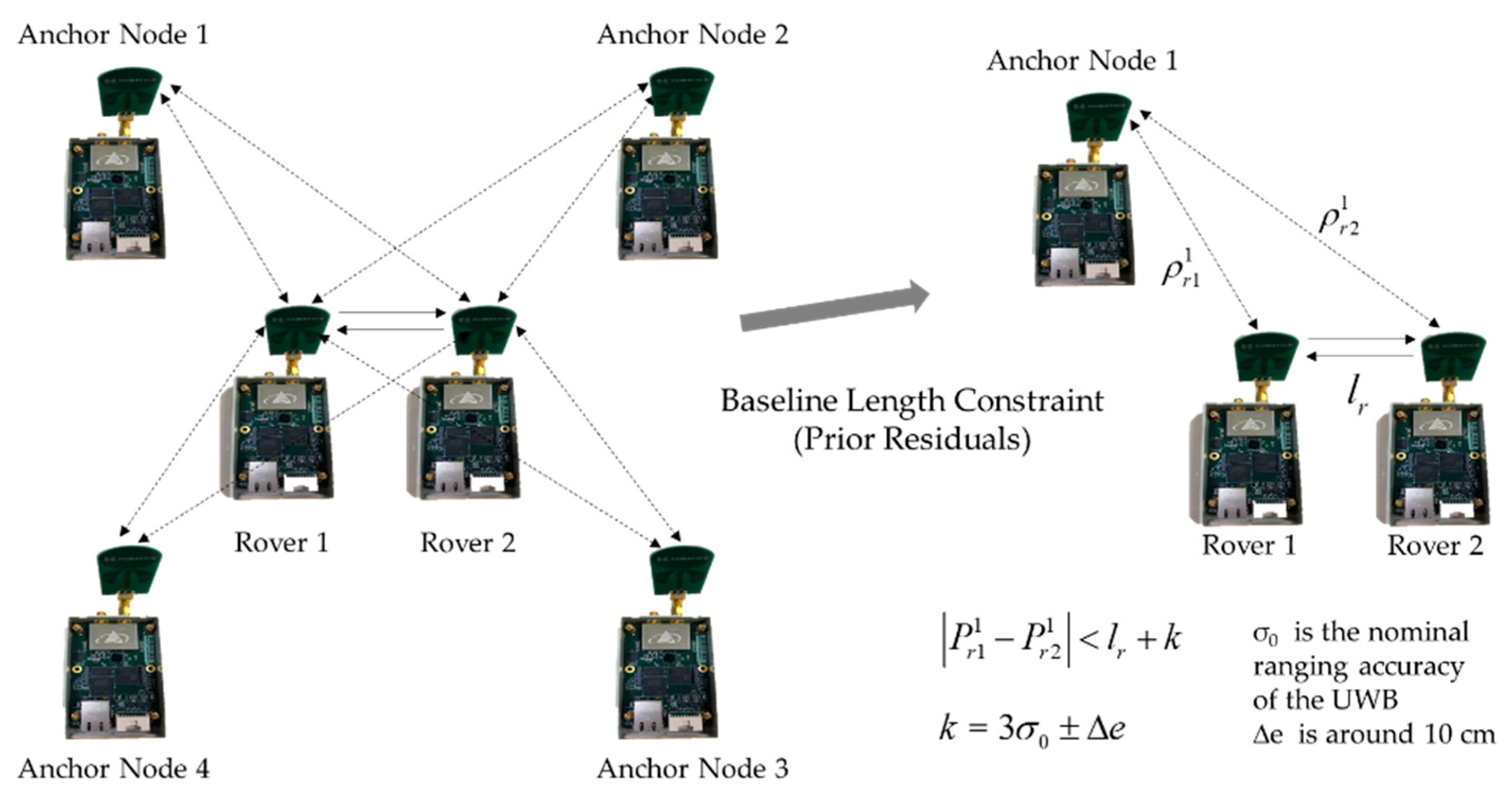
For large random and gross errors, two rover stations are introduced and the DD UWB positioning method with additional baseline constraints is proposed for positioning quality control.

The experimental results show that the proposed method can eliminate the systematic error effectively and reach the high accuracy of the positioning results. After adopting the baseline constraint, gross errors and large random errors are eliminated as well. The experimental results are summarized as follows:

(1)

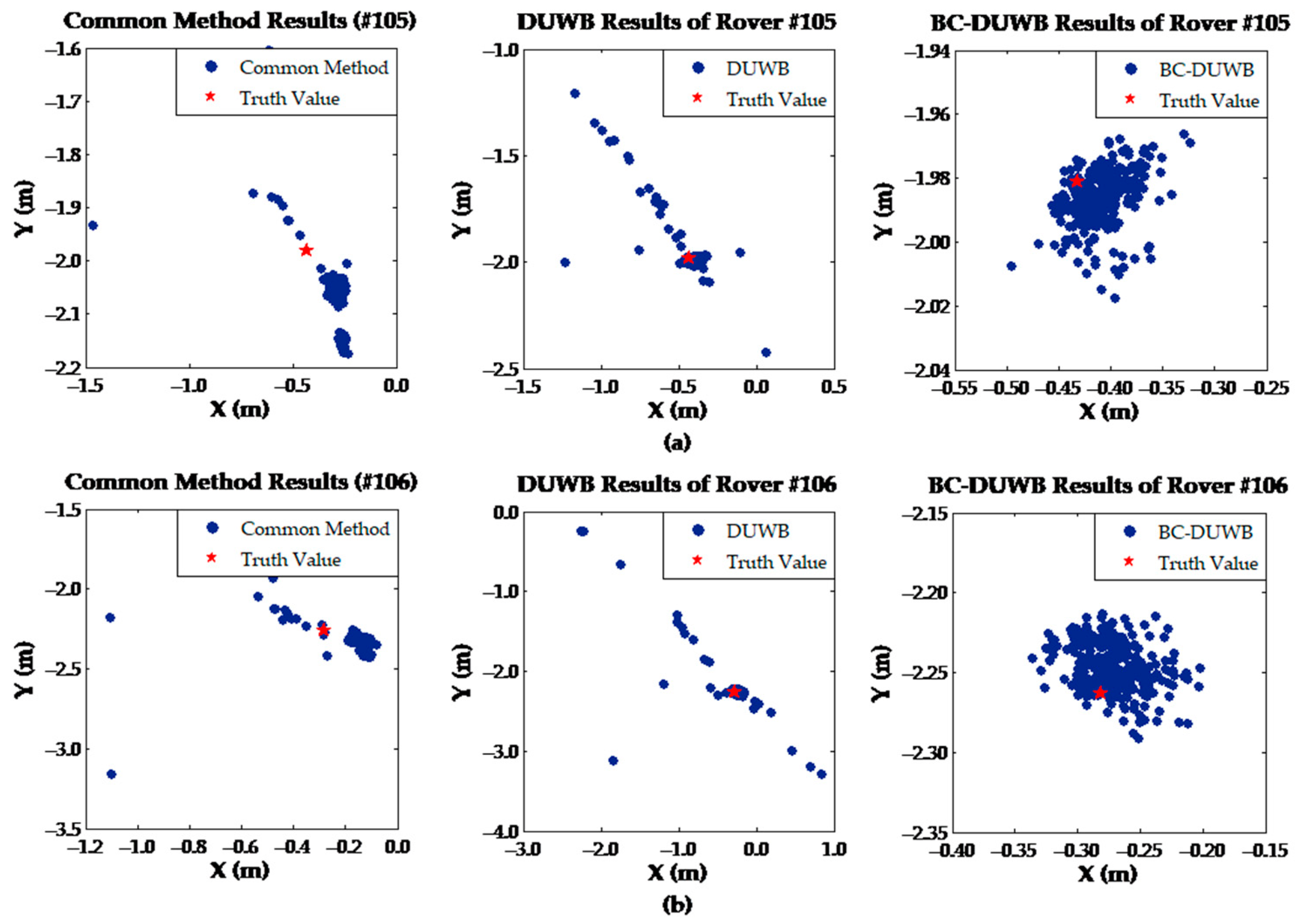
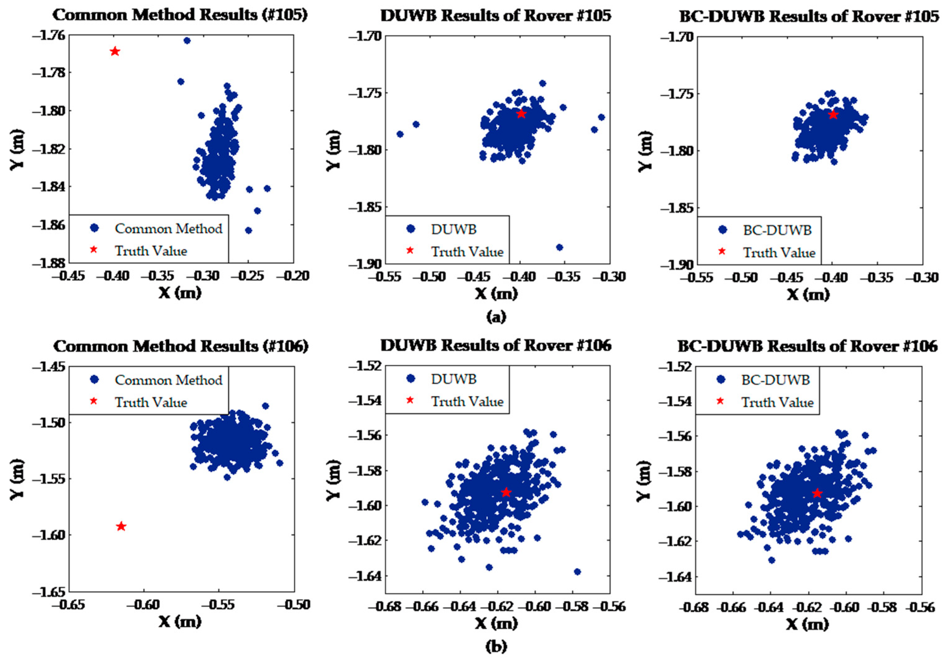
The positioning precision of two rover stations in static experiments is more than 80% higher than that of the common method. When the data quality is poor, the positioning precision can reach about 3.4 cm. The positioning precision can reach 2.0 cm when the data quality is good, which further illustrates the robustness of the proposed method.

(2)

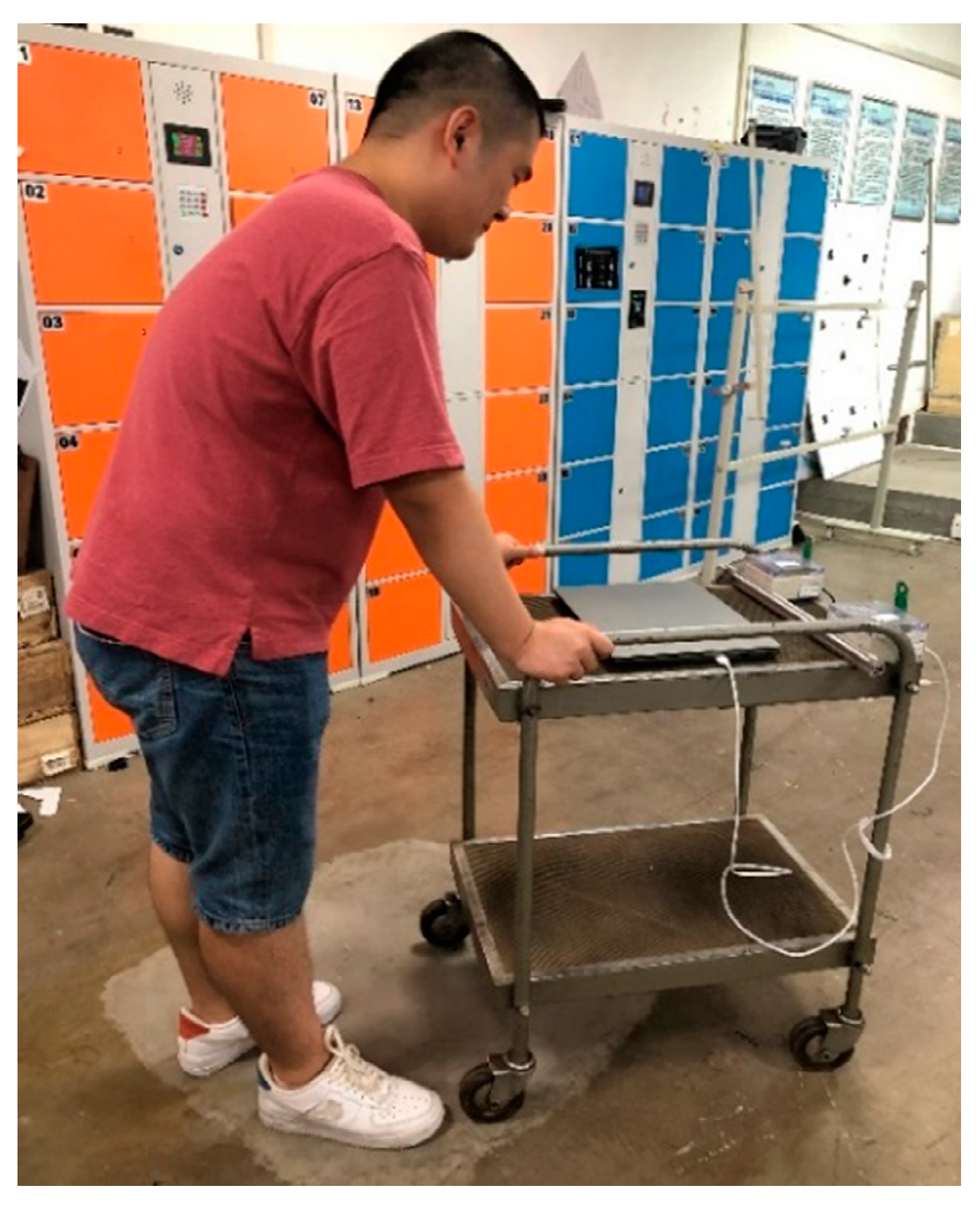
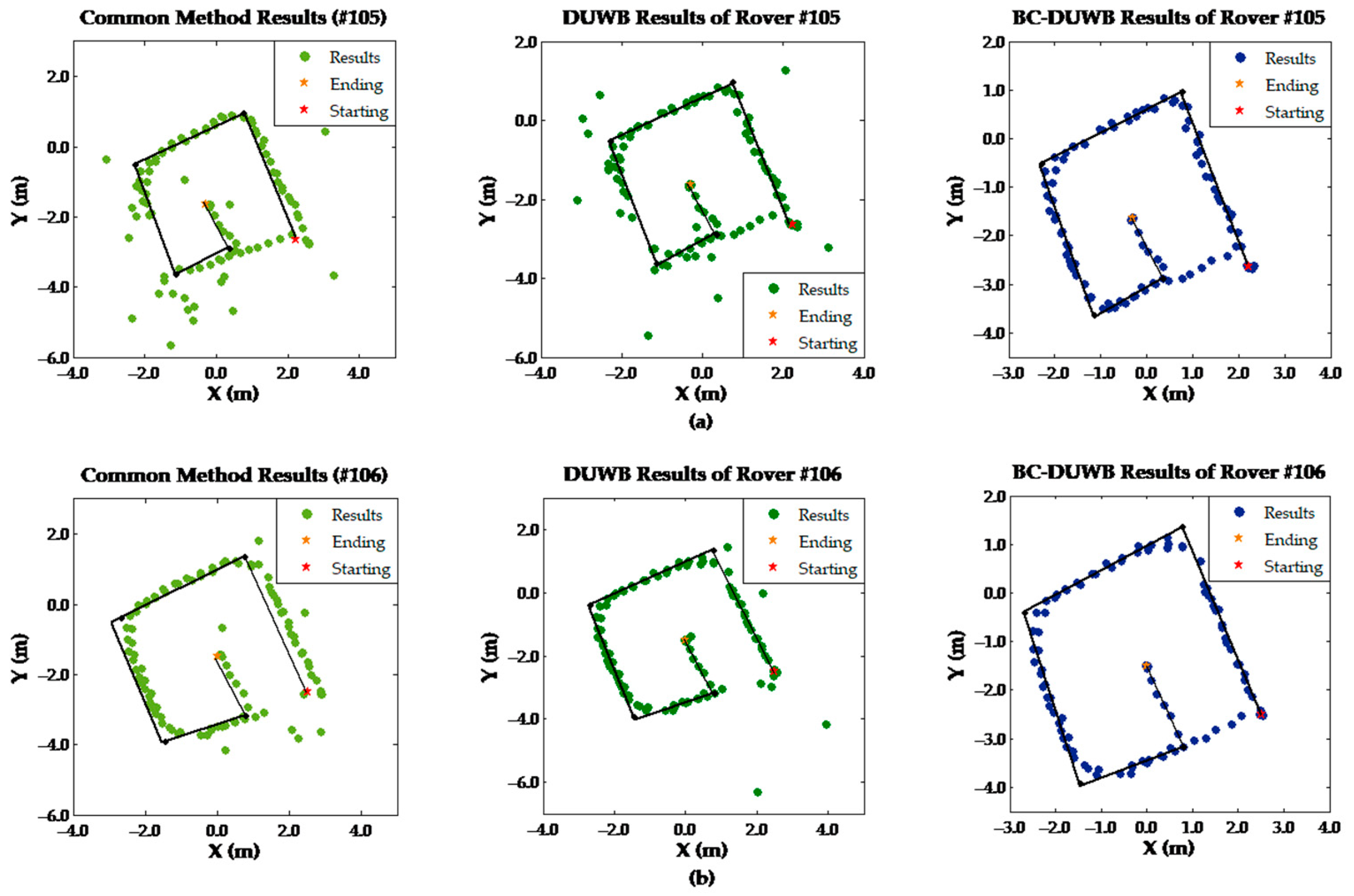
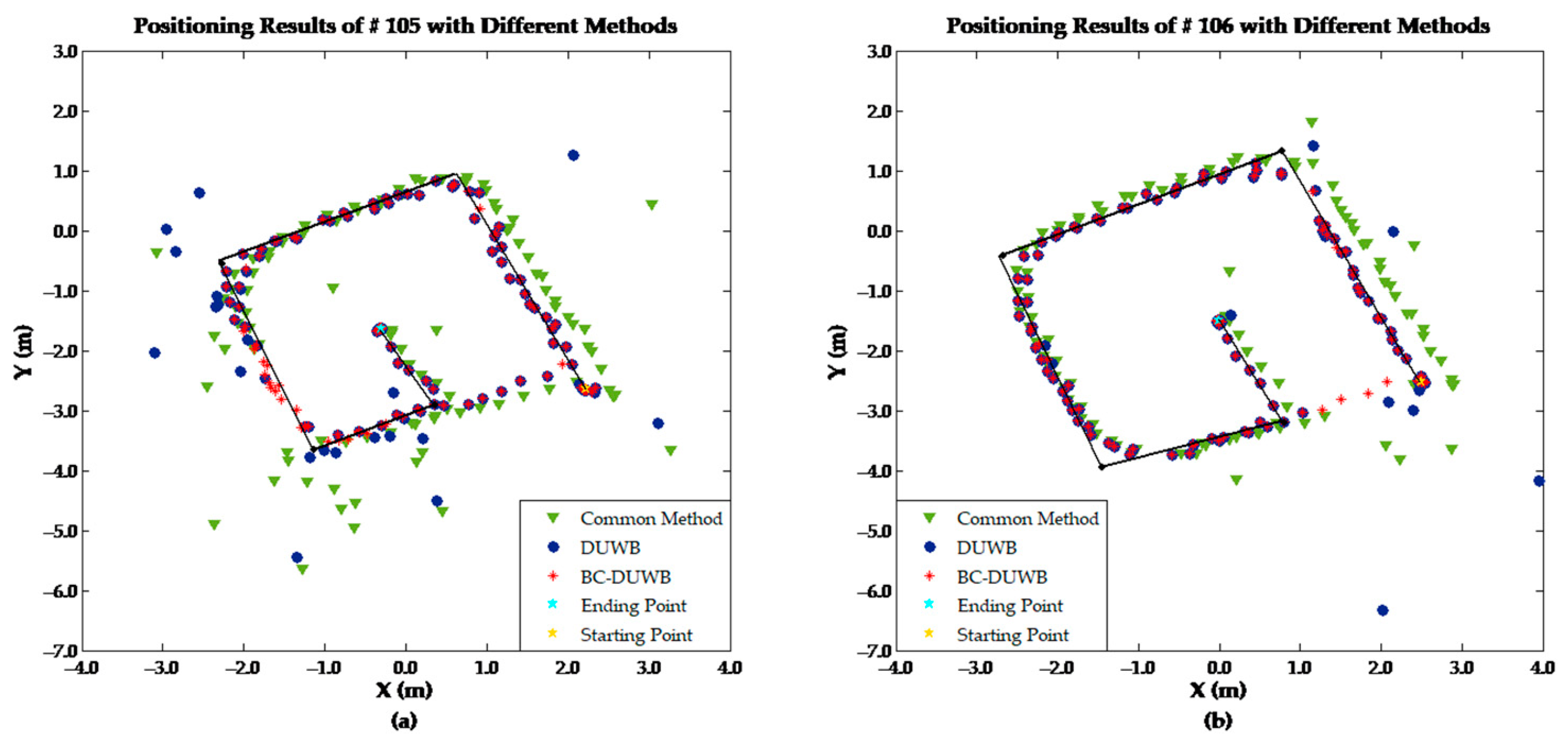
In the dynamic experiment, the results of BC-DUWB are not only closer to the reference trajectory than adopting the common method, but the coordinates of the starting point and ending point are almost consistent with the truth value. Furthermore, the gross error and large random error are also eliminated, so that the maximum deviation is less than 5 cm.

However, there are still some deficiencies in this article, such as the fact that the principle of anchor nodes arrangement has not been studied. Therefore, various arrangement methods will be compared in the near future. In addition, the trolley velocity in the dynamic experiment is slow, and lacks tests for fast-moving scenes. The dynamic analysis model needs to be improved to adapt to the fast-moving application scenarios. UWB has a strong penetration ability in some cases, such as in wood and stones, and the penetration error can be corrected by modeling. However, it has a weak ability to penetrate water and metal. Therefore, of the expected errors in this paper, other UWB errors including penetration error and NLOS will be the next research focus. These factors will affect the validity of the results. Since the main purpose of this paper is to verify the feasibility of the method, there is no modeling of penetration errors or NLOS in the algorithm. For the applicability of the algorithm, the algorithm should be optimized to adapt to the NLOS environment in the future. Furthermore, the anchor nodes will be placed in different rooms and conduct networking experiments in practical environments, such as large scene factories and underground projects.

References

1. Zhao, Y.; Guo, J.; Zou, J.; Zhang, P.; Zhang, D.; Li, X.; Huang, G.; Yang, F. A Holistic Approach to Guarantee the Reliability of Positioning Based on Carrier Phase for Indoor Pseudolite. Appl. Sci. 2020, 10, 1199. [Google Scholar] [CrossRef] [Green Version]
2. Wang, C.; Ning, Y.; Li, X.; Li, H. A Robust Unscented Kalman Filter applied to Ultra-wideband Positioning. Int. J. Image Data Fusion 2020, 11, 308–330. [Google Scholar] [CrossRef]
3. Albaidhani, A.; Morell, A.; Vicario, J.L. Anchor selection for UWB indoor positioning. Trans. Emerg. Telecommun. Technol. 2019, 30, e3598. [Google Scholar] [CrossRef]
4. Lin, Y.; Zhang, G. The optimal arrangement of four laser tracking interferometers in 3D coordinate measuring system based on multilateration. In Proceedings of the IEEE International Symposium on Virtual Environments, Human-Computer Interfaces and Measurement Systems, (VECIMS’03), Lugano, Switzerland, 27–29 July 2003; pp. 138–143. [Google Scholar]
5. Monica, S.; Ferrari, G. UWB-based localization in large indoor scenarios: Optimized placement of anchor nodes. IEEE Trans. Aerosp. Electron. Syst. 2015, 51, 987–999. [Google Scholar] [CrossRef]
6. Chen, Y.Y.; Huang, S.P.; Wu, T.W.; Tsai, W.T.; Liou, C.Y.; Mao, S.G. UWB System for Indoor Positioning and Tracking with Arbitrary Target Orientation, Optimal Anchor Location, and Adaptive NLOS Mitigation. IEEE Trans. Veh. Technol. 2020, 69, 9304–9314. [Google Scholar] [CrossRef]
7. Li, T.Y.; Duan, F.J.; Liang, C.J.; Jiang, J.J.; Fu, X.; Wang, Q.; Huang, H.X.; Wei, Q.F. A high-precision unmanned aerial vehicle positioning system based on ultra-wideband technology. Meas. Sci. Technol. 2021, 32, 055101. [Google Scholar] [CrossRef]
8. Pan, H.; Qi, X.; Liu, M.; Liu, L. Map-aided and UWB-based anchor placement method in indoor localization. Neural Comput. Appl. 2021, 33, 11845–11859. [Google Scholar] [CrossRef]
9. Wang, S.; Wang, S.; Liu, W.; Tian, Y. A Study on the Optimization Nodes Arrangement in UWB Localization. Measurement 2020, 163, 108056. [Google Scholar] [CrossRef]
10. Wang, M.; Chen, Z.; Zhou, Z.; Fu, J.; Qiu, H. Analysis of the Applicability of Dilution of Precision in the Base Station Configuration Optimization of Ultrawideband Indoor TDOA Positioning System. IEEE Access 2020, 8, 225076–225087. [Google Scholar] [CrossRef]
11. Tennina, S.; Di Renzo, M.; Graziosi, F.; Santucci, F. Locating zigbee® nodes using the ti® s cc2431 location engine: A testbed platform and new solutions for positioning estimation of wsns in dynamic indoor environments. In Proceedings of the ACM International Workshop on Mobile Entity Localization and Tracking in GPS-Less Environments, San Francisco, CA, USA, 19 September 2008. [Google Scholar]
12. Geng, C.; Hu, M.; Qing, Z. The design of an indoor high-precision multi-source wireless positioning system in B5G environment. Phys. Commun. 2020, 43, 101232. [Google Scholar]
13. Graichen, T.; Richter, J.; Schmidt, R.; Heinkel, U. Improved Indoor Positioning by Means of Occupancy Grid Maps Automatically Generated from OSM Indoor Data. ISPRS Int. J. Geo-Inf. 2021, 10, 216. [Google Scholar] [CrossRef]
14. Krapež, P.; Munih, M. Anchor Calibration for Real-Time-Measurement Localization Systems. IEEE Trans. Instrum. Meas. 2020, 69, 9907–9917. [Google Scholar] [CrossRef]
15. Wang, J.; Wang, M.; Yang, D.; Liu, F.; Wen, Z. UWB positioning algorithm and accuracy evaluation for different indoor scenes. Int. J. Image Data Fusion 2021, 2, 1–23. [Google Scholar]
16. Li, Z.; Zhao, L.; Wang, Y.; Yang, Z.; Liu, Z.; Wang, C. Variance optimization of UWB observation based on map matching for PPP/INS/UWB tightly coupled positioning. Meas. Sci. Technol. 2021, 32, 025007. [Google Scholar] [CrossRef]
17. Nguyen, T.H.; Nguyen, T.M.; Xie, L. Range-Focused Fusion of Camera-IMU-UWB for Accurate and Drift-Reduced Localization. IEEE Robot. Autom. Lett. 2021, 6, 1678–1685. [Google Scholar] [CrossRef]
18. Li, X.; Wang, Y. The IMU/UWB Fusion Positioning Algorithm Based on a Particle Filter. ISPRS Int. J. Geo-Inf. 2017, 6, 235. [Google Scholar]
19. Li, M.G.; Zhu, H.; You, S.Z.; Tang, C.Q. UWB-Based Localization System Aided with Inertial Sensor for Underground Coal Mine Applications. IEEE Sens. J. 2020, 20, 6652–6669. [Google Scholar] [CrossRef]
20. Guo, S.; Zhang, Y.; Gui, X.; Han, L. An Improved PDR/UWB Integrated System for Indoor Navigation Applications. IEEE Sens. J. 2020, 20, 8046–8061. [Google Scholar] [CrossRef]
21. Wang, Y.; Li, X. Graph-Optimization-Based ZUPT/UWB Fusion Algorithm. ISPRS Int. J. Geo-Inf. 2018, 7, 18. [Google Scholar] [CrossRef] [Green Version]
22. Zhang, Y.; Tan, X.; Zhao, C. UWB/INS Integrated Pedestrian Positioning for Robust Indoor Environments. IEEE Sens. J. 2020, 20, 14401–14409. [Google Scholar] [CrossRef]
23. Lutz, P.; Schuster, M.J.; Steidle, F. Visual-inertial SLAM aided estimation of anchor poses and sensor error model parameters of UWB radio modules. In Proceedings of the 19th International Conference on Advanced Robotics (ICAR), Belo Horizonte, Brazil, 2–6 December 2019; pp. 739–746. [Google Scholar]
24. Bharadwaj, R.; Koul, S.K. Study of the Influence of Human Subject on the Indoor Channel Using Compact UWB Directive/Omni-Directional Antennas for Wireless Sensor Network Applications. Ad Hoc Netw. 2021, 118, 102621. [Google Scholar] [CrossRef]
25. Cao, B.; Wang, S.; Ge, S.; Liu, W. Improving Positioning Accuracy of UWB in Complicated Underground NLOS Scenario Using Calibration, VBUKF, and WCA. IEEE Trans. Instrum. Meas. 2021, 70, 8501013. [Google Scholar] [CrossRef]
26. Yang, X.; Wang, J.; Song, D.; Feng, B.; Ye, H. A Novel NLOS Error Compensation Method Based IMU for UWB Indoor Positioning System. IEEE Sens. J. 2021, 21, 11203–11212. [Google Scholar] [CrossRef]
27. Zhang, Y.; Duan, L. A phase-difference-of-arrival assisted ultra-wideband positioning method for elderly care. Measurement 2021, 170, 108689. [Google Scholar] [CrossRef]
28. Cui, Z.; Liu, T.; Tian, S.; Xu, R.; Cheng, J. Non-Line-of-Sight Identification for UWB Positioning Using Capsule Networks. IEEE Commun. Lett. 2020, 24, 2187–2190. [Google Scholar] [CrossRef]
29. Jiang, C.; Shen, J.; Chen, S.; Chen, Y.; Liu, D.; Bo, Y. UWB NLOS/LOS Classification Using Deep Learning Method. IEEE Commun. Lett. 2020, 24, 2226–2230. [Google Scholar] [CrossRef]
30. Ridolfi, M.; Fontaine, J.; Van Herbruggen, B.; Joseph, W.; Hoebeke, J.; De Poorter, E. UWB anchor nodes self-calibration in NLOS conditions: A machine learning and adaptive PHY error correction approach. Wirel. Netw. 2021, 27, 3007–3023. [Google Scholar] [CrossRef]
31. Yu, K.; Wen, K.; Li, Y.; Zhang, S.; Zhang, K. A Novel NLOS Mitigation Algorithm for UWB Localization in Harsh Indoor Environments. IEEE Trans. Veh. Technol. 2018, 68, 686–699. [Google Scholar] [CrossRef]
32. Cui, Z.; Gao, Y.; Hu, J.; Tian, S.; Cheng, J. LOS/NLOS Identification for Indoor UWB Positioning Based on Morlet Wavelet Transform and Convolutional Neural Networks. IEEE Commun. Lett. 2021, 25, 879–882. [Google Scholar] [CrossRef]
33. Wang, C.; Han, H.; Wang, J.; Yu, H.; Yang, D. A Robust Extended Kalman Filter Applied to Ultra wide band Positioning. Math. Probl. Eng. 2020, 2020, 1809262. [Google Scholar]
34. Yuan, D.; Zhang, J.; Wang, J.; Cui, X.; Liu, F.; Zhang, Y. Robustly Adaptive EKF PDR/UWB Integrated Navigation Based on Additional Heading Constraint. Sensors 2021, 21, 4390. [Google Scholar] [CrossRef] [PubMed]
35. Yin, H.; Xia, W.; Zhang, Y.; Shen, L. UWB-based indoor high precision localization system with robust unscented Kalman filter. In Proceedings of the IEEE International Conference on Communication Systems (ICCS), Shenzhen, China, 14–16 December 2016. [Google Scholar]
36. Xia, B.; Liu, T.; Ding, T.; Wang, Z. An Improved PSO Localization Algorithm for UWB Sensor Networks. Wirel. Pers. Commun. 2021, 117, 2207–2223. [Google Scholar] [CrossRef]
37. Mautz, R. Indoor Positioning Technologies; Südwestdeutscher Verlag für Hochschulschriften: Zurich, Switzerland, 2012. [Google Scholar]
38. Decawave. DWM1000 Module. Available online: https://www.decawave.com/product/dwm1000-module (accessed on 10 September 2021).
39. Wen, L.; Han, J.; Song, L.; Zhang, Q.; Li, K.; Li, Z.; Zhang, W.; Zhang, B.; You, X.; Sung, Y.; et al. An Automated Real-Time Localization System in Highway and Tunnel Using UWB DL-TDoA Technology. Wirel. Commun. Mob. Comput. 2020, 2020, 8877654. [Google Scholar] [CrossRef]
40. Hasan, H.S.; Abidin, M.S.Z.; Mahmud, M.S.A.; Said, M.F.M. Ultra-Wideband based on Automated Guided Vehicle for Localization. Int. Trans. J. Eng. Manag. Appl. Sci. Technol. 2021, 12, 1–8. [Google Scholar]
41. Lau, L.; Quan, Y.; Wan, J.; Zhou, N.; Wen, C.; Qian, N.; Jing, F. An Autonomous Ultra-Wide Band-Based Attitude and Position Determination Technique for Indoor Mobile Laser Scanning. ISPRS Int. J. Geo-Inf. 2018, 7, 155. [Google Scholar] [CrossRef] [Green Version]
42. Cellmer, S.; Wielgosz, P.; Rzepecka, Z. Modified ambiguity function approach for GPS carrier phase positioning. J. Géod. 2010, 84, 267–275. [Google Scholar] [CrossRef]
43. TIME DOMAIN. 320-0320D RangeNet User Guide. Available online: https://manualzz.com/doc/29413471/320-0320d-rangenet-user-guide (accessed on 10 September 2021).
Figure 1. TW-TOF schematic diagram.
Ijgi 10 00634 g001
Figure 2. Schematic diagram of prior baseline constraint.
Ijgi 10 00634 g002
Figure 3. Schematic diagram of the proposed method BC-DUWB.
Ijgi 10 00634 g003
Figure 4. Anchor nodes arrangement in our laboratory.
Ijgi 10 00634 g004
Figure 5. Plane location distribution of anchor nodes.
Ijgi 10 00634 g005
Figure 6. The ranging observations between anchor node 104 and #107/#108.
Ijgi 10 00634 g006
Figure 7. Anchor nodes arrangement in our laboratory.
Ijgi 10 00634 g007
Figure 8. (a) The difference of ranging observations (from #109 to two rovers); (b) The difference of ranging observations (from #110 to two rovers).
Ijgi 10 00634 g008
Figure 9. (a) The positioning results of rover #105 with different methods (Test 1); (b) The positioning results of rover #106 with different methods (Test 1).
Ijgi 10 00634 g009
Figure 10. (a) The difference of ranging observations (from #107 to two rovers); (b) The difference of ranging observations (from #108 to two rovers).
Ijgi 10 00634 g010
Figure 11. (a) The positioning results of rover #105 with different methods (Test 2); (b) The positioning results of rover #106 with different methods (Test 2).
Ijgi 10 00634 g011
Figure 12. The location of the two rover stations and the trolley in Test 3.
Ijgi 10 00634 g012
Figure 13. (a) The positioning results of rover #105 with different methods (Test 3); (b) The positioning results of rover #106 with different methods (Test 3).
Ijgi 10 00634 g013
Figure 14. (a) The positioning results of rover #105 with different methods (Test 3); (b) The positioning results of rover #106 with different methods (Test 3); (c) GDOP and the number of available anchors during #105 movement; (d) GDOP and the number of available anchors during #106 movement.
Ijgi 10 00634 g014aIjgi 10 00634 g014b