Comparison of Ensemble Machine Learning Methods for Soil Erosion Pin Measurements


Abstract
:1. Introduction
2. Methods
2.1. Bagging
2.2. Boosting
2.3. Stacking
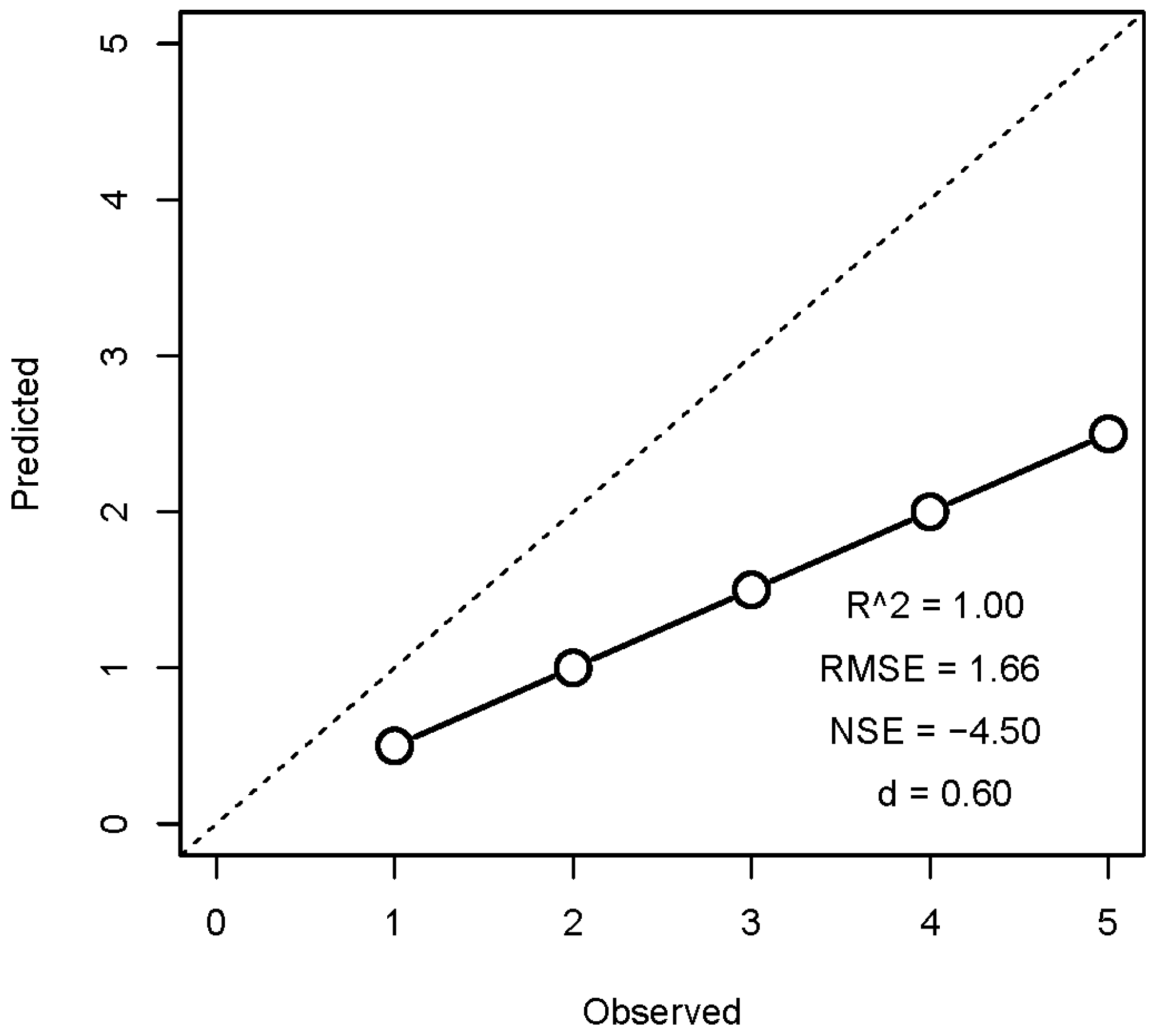
2.4. Model Assessment
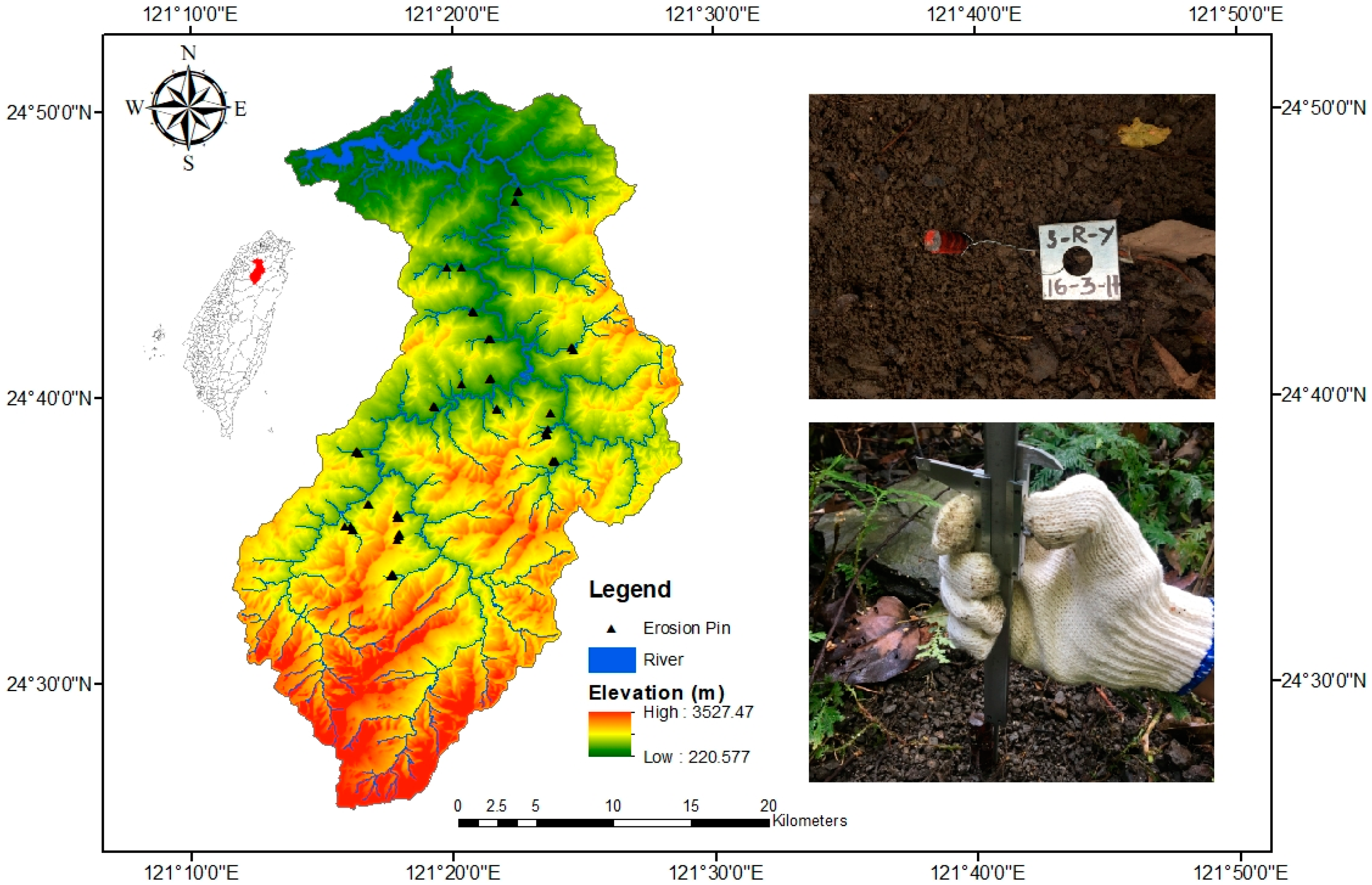
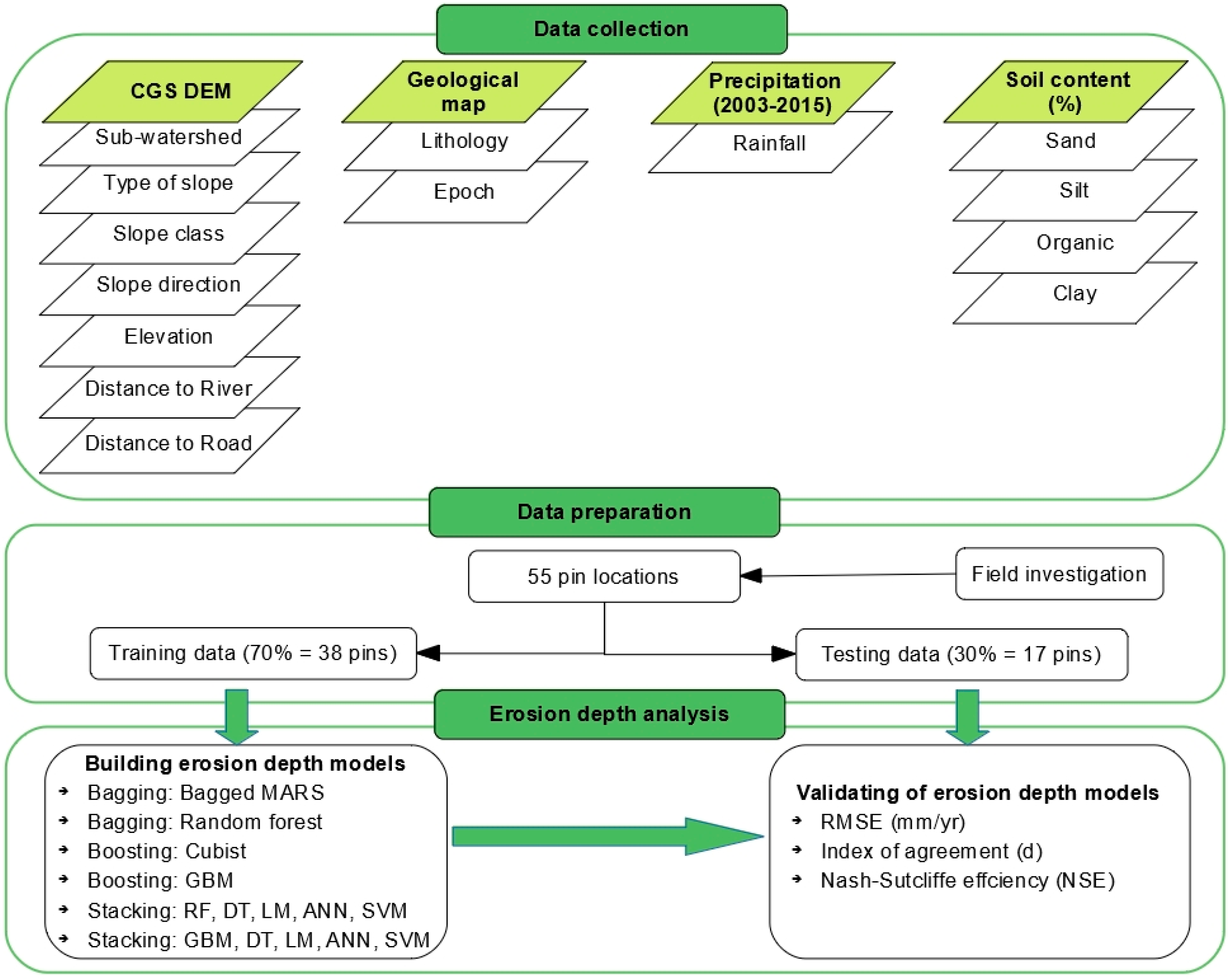
2.5. Study Area
3. Results and Discussion
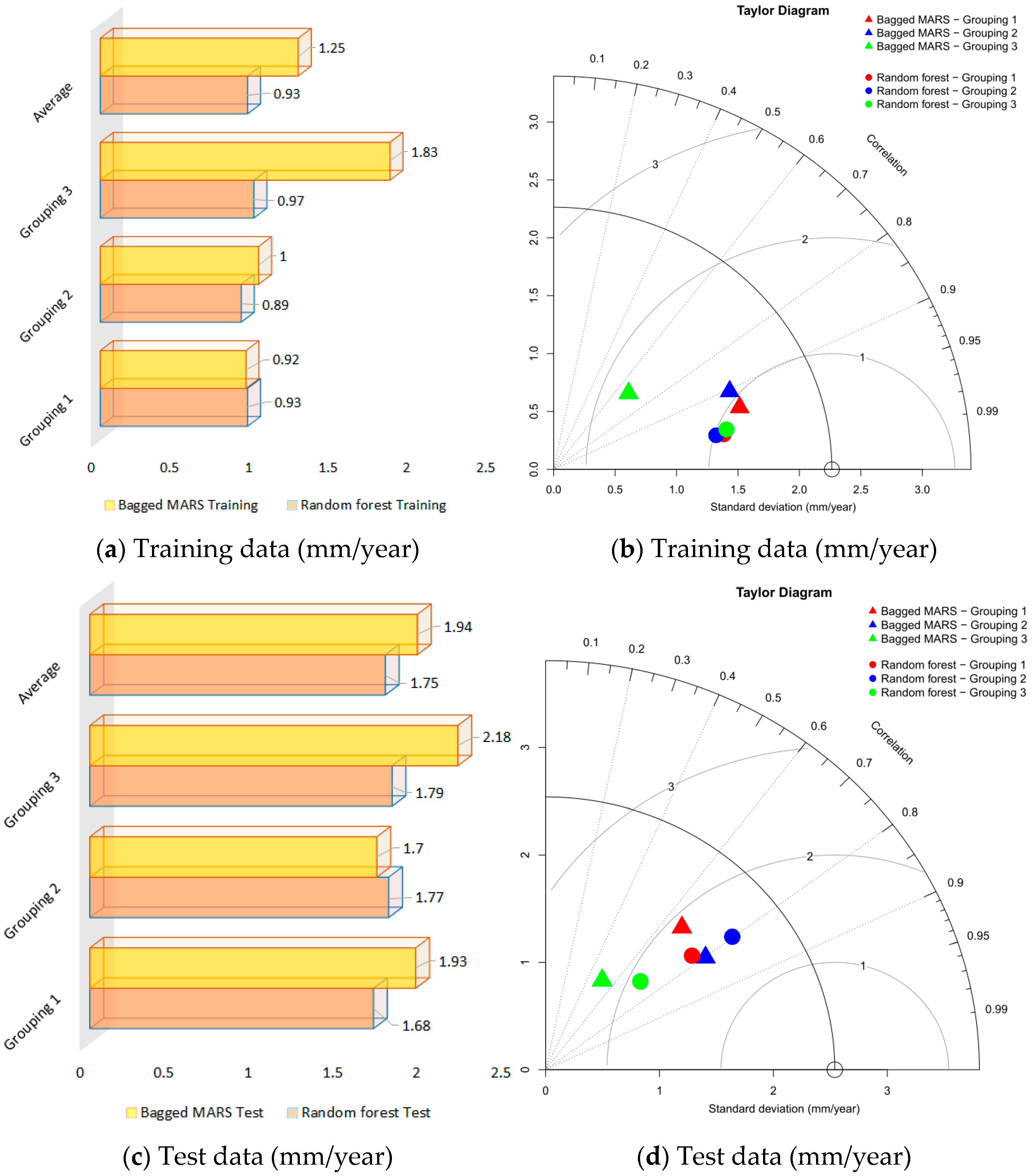
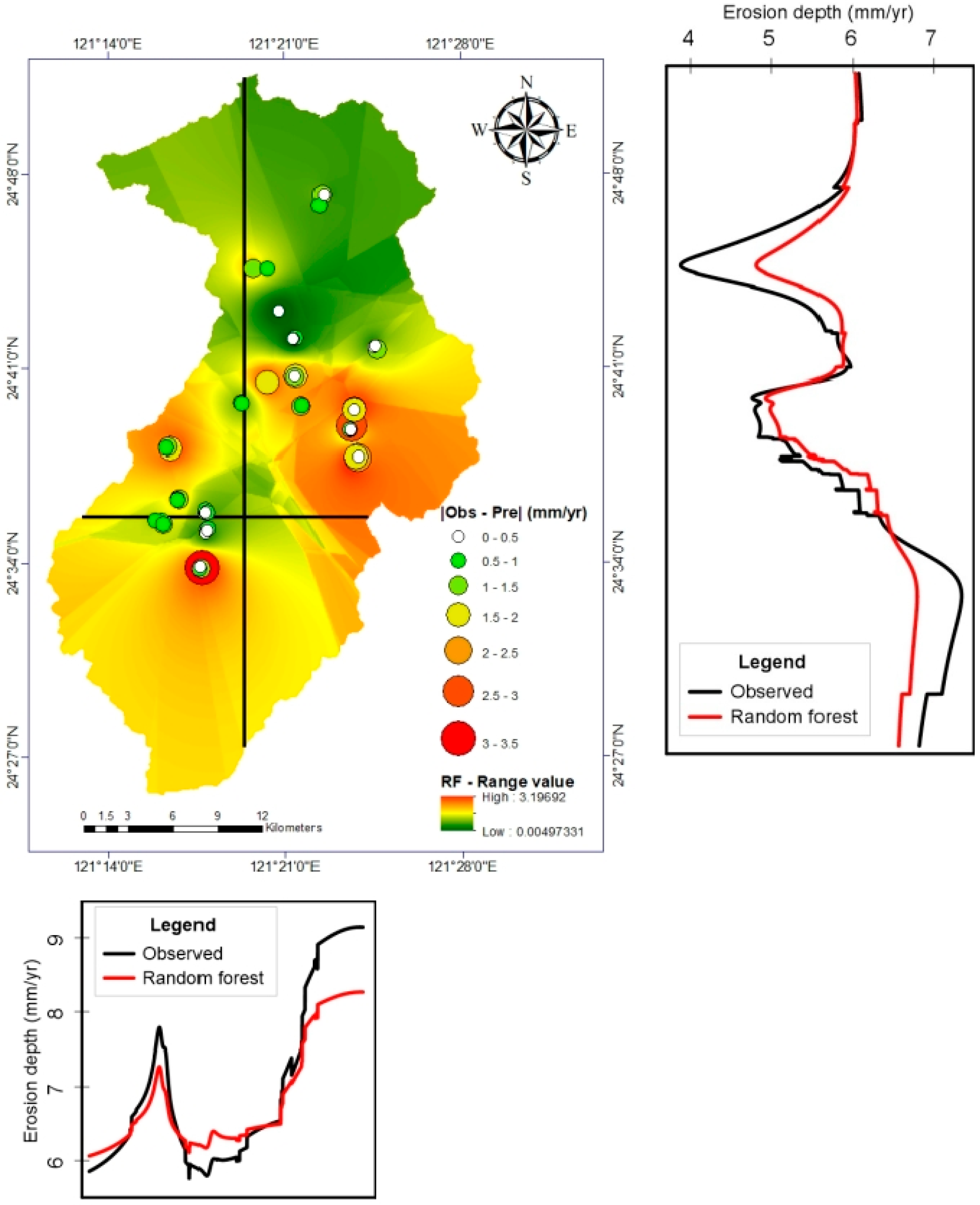
3.1. Bagging
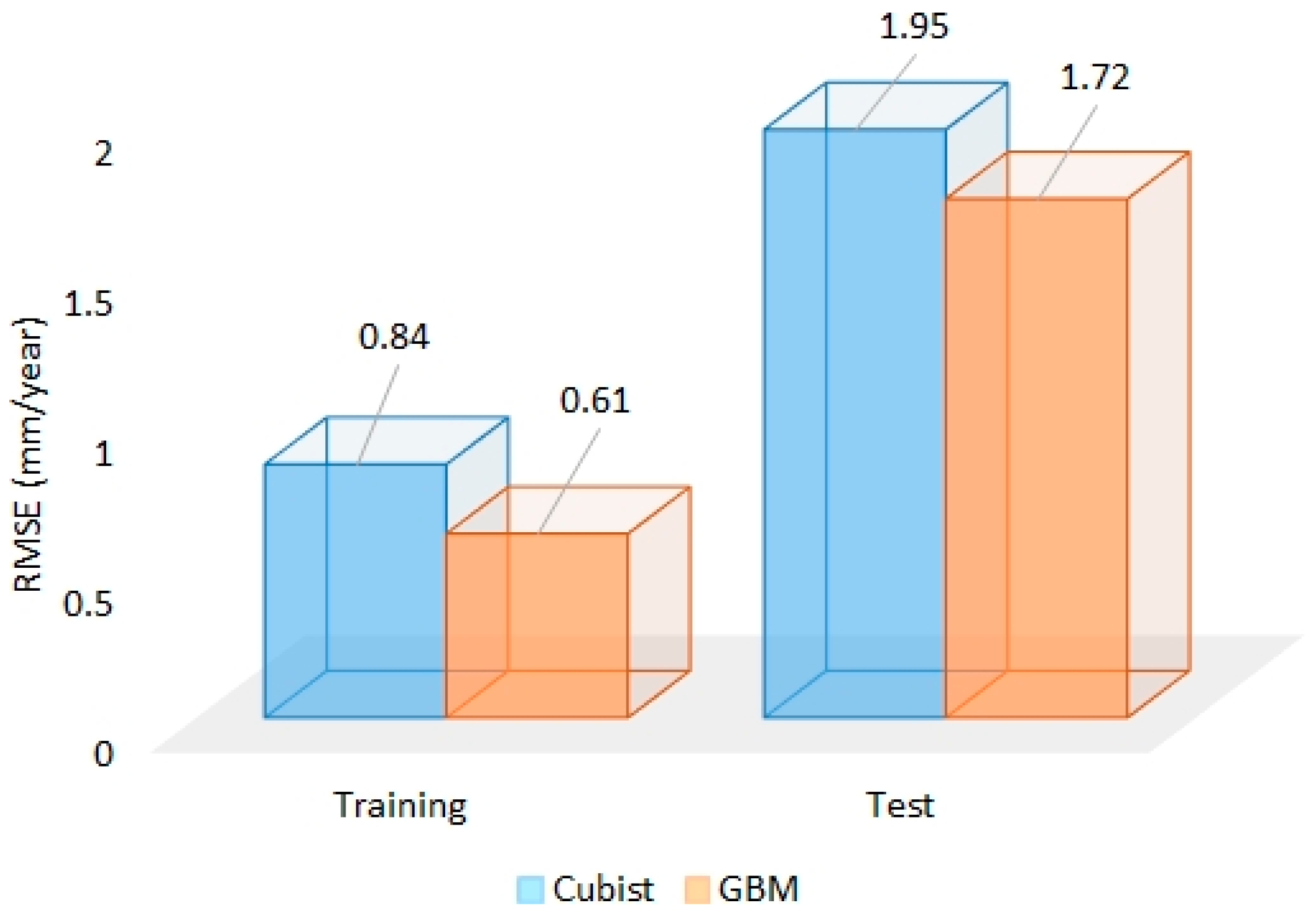
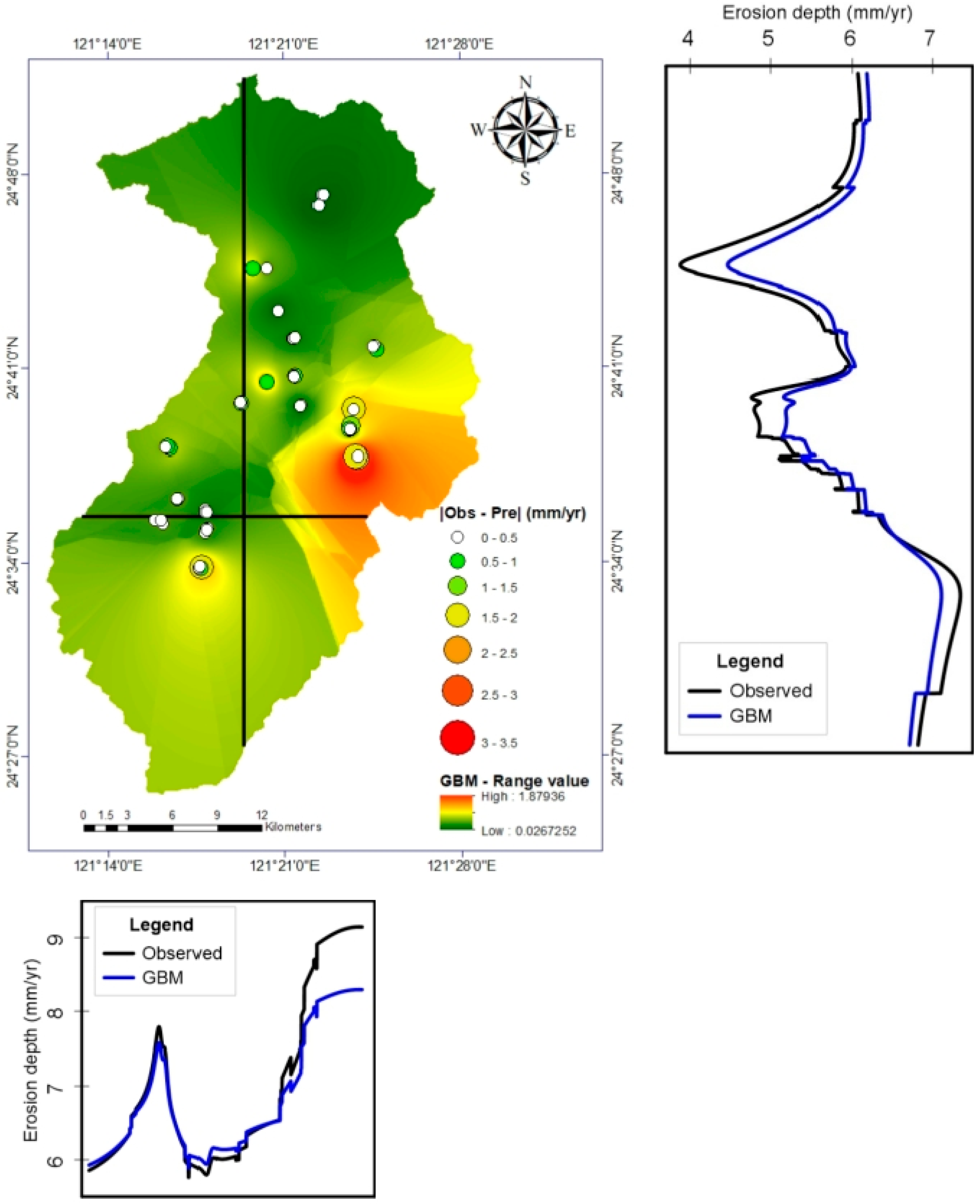
3.2. Boosting
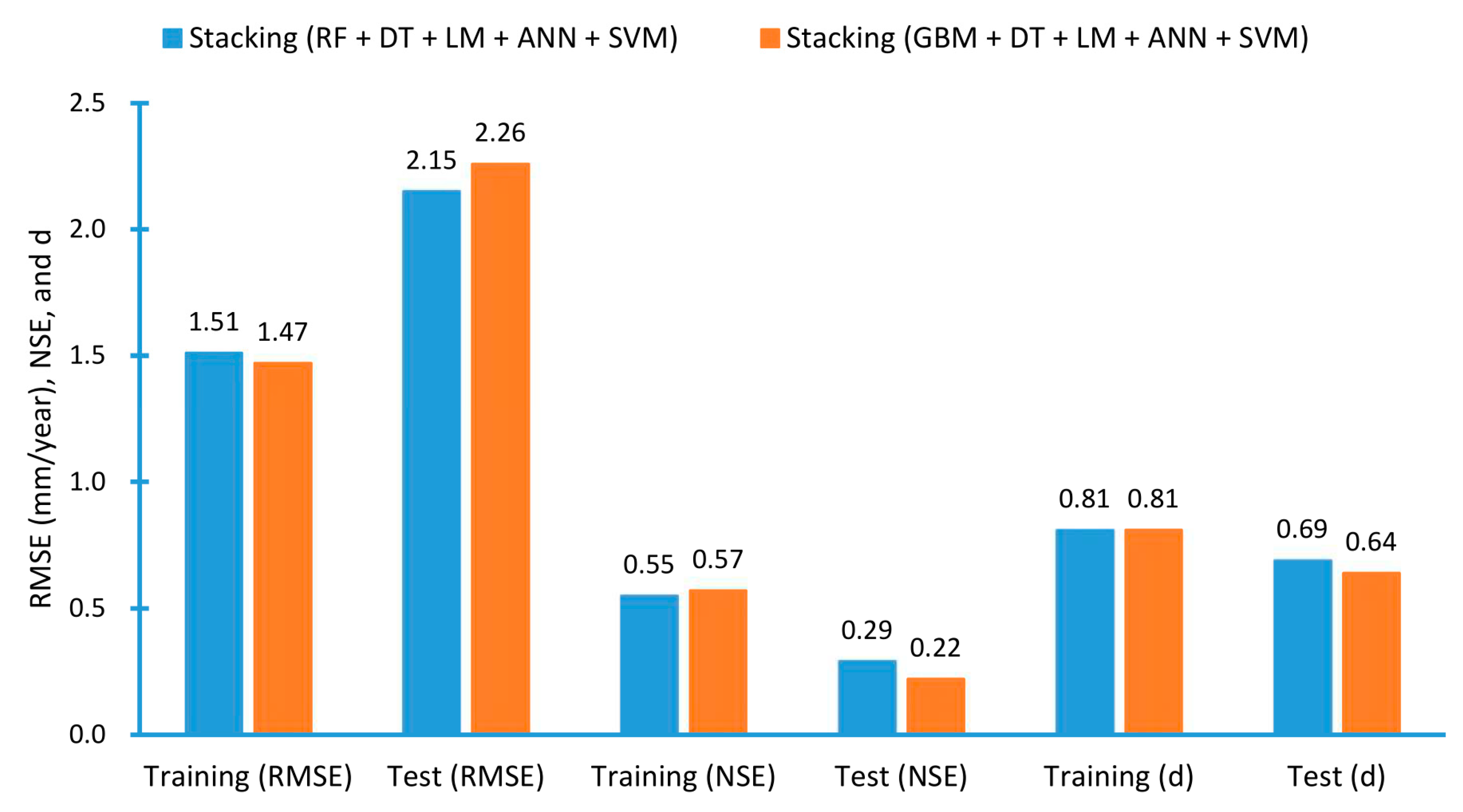
3.3. Stacking
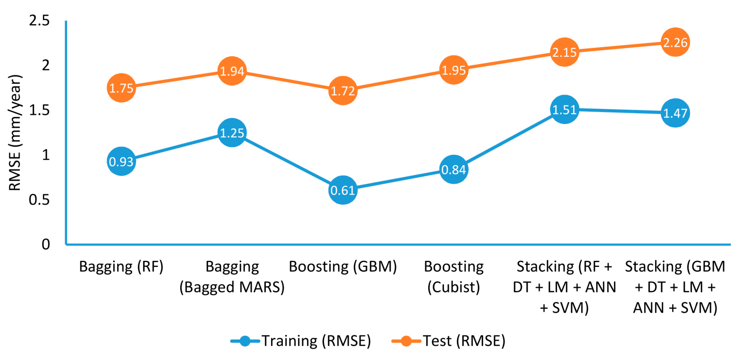
3.4. Comparison of Ensemble Models
- Training: GBM > Cubist > RF > bagged MARS > Stacking (GBM) > Stacking (RF)
- Test: GBM > RF > bagged MARS > Cubist > Stacking (RF) > Stacking (GBM)
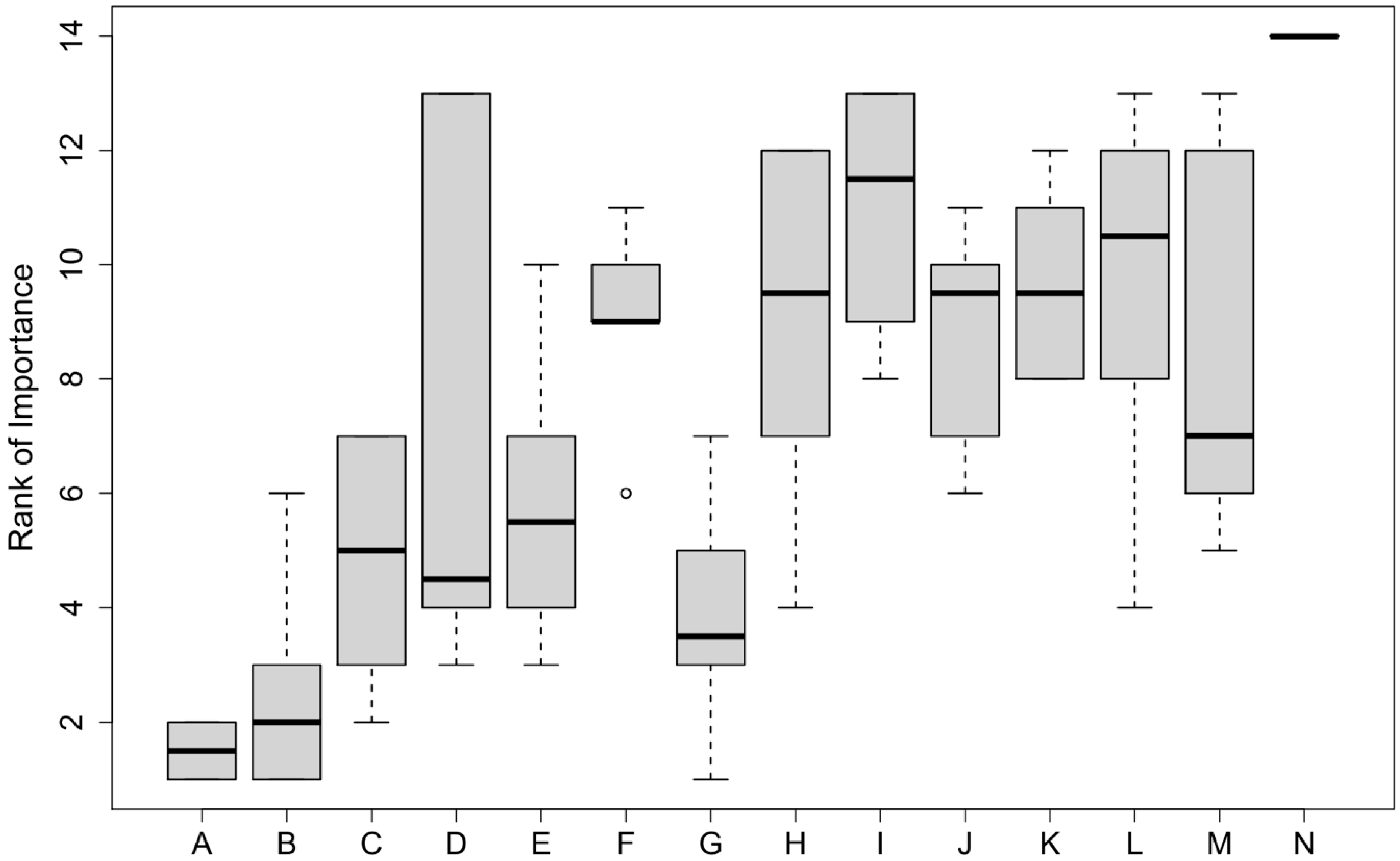
3.5. Model Predictions and Factor Importance
4. Conclusions
Author Contributions
Funding
Institutional Review Board Statement
Informed Consent Statement
Data Availability Statement
Conflicts of Interest
References
- Ruiz-Sinoga, J.D.; Martínez-Murillo, J.F. Hydrological response of abandoned agricultural soils along a climatological gradient on metamorphic parent material in southern Spain. Earth Surf. Process. Landf. 2009, 34, 2047–2056. [Google Scholar] [CrossRef]
- García-Ruiz, J.M. The effects of land uses on soil erosion in Spain: A review. Catena 2010, 81, 1–11. [Google Scholar] [CrossRef]
- Morgan, R.P.C. Soil Erosion and Conservation; John Wiley & Sons: Hoboken, NJ, USA, 2009. [Google Scholar]
- Islam, R.; Jaafar, W.Z.W.; Hin, L.S.; Osman, N.; Hossain, A.; Mohd, N.S. Development of an intelligent system based on ANFIS model for predicting soil erosion. Environ. Earth Sci. 2018, 77, 186. [Google Scholar] [CrossRef]
- Lal, R. Soil degradation by erosion. Land Degrad. Dev. 2001, 12, 519–539. [Google Scholar] [CrossRef]
- Borrelli, P.; Alewell, C.; Alvarez, P.; Anache, J.A.A.; Baartman, J.; Ballabio, C.; Bezak, N.; Biddoccu, M.; Cerdà, A.; Chalise, D.; et al. Soil erosion modelling: A global review and statistical analysis. EarthArxiv 2020. [Google Scholar] [CrossRef]
- Yeh, S.-C.; Wang, C.-A.; Yu, H.-C. Simulation of soil erosion and nutrient impact using an integrated system dynamics model in a watershed in Taiwan. Environ. Model. Softw. 2006, 21, 937–948. [Google Scholar] [CrossRef]
- Fan, J.-C.; Wu, M.-F. Effects of soil strength, texture, slope steepness and rainfall intensity on interrill erosion of some soils in Taiwan. In Proceedings of the 10th International Soil Conservation Organization Meeting, Purdue University, USDA-ARS National Soil Erosion Research Laboratory, W. Lafayette, IN, USA, 24–29 May 1999. [Google Scholar]
- Lo, K.F.A. Erosion assessment of large watersheds in Taiwan. J. Soil Water Conserv. 1995, 50, 180–183. [Google Scholar]
- Chiu, Y.-J.; Chang, K.-T.; Chen, Y.-C.; Chao, J.-H.; Lee, H.-Y. Estimation of soil erosion rates in a subtropical mountain watershed using 137Cs radionuclide. Nat. Hazards 2011, 59, 271–284. [Google Scholar] [CrossRef]
- Chen, W.; Li, D.-H.; Yang, K.-J.; Tsai, F.; Seeboonruang, U. Identifying and comparing relatively high soil erosion sites with four DEMs. Ecol. Eng. 2018, 120, 449–463. [Google Scholar] [CrossRef]
- Liu, Y.-H.; Li, D.-H.; Chen, W.; Lin, B.-S.; Seeboonruang, U.; Tsai, F. Soil Erosion Modeling and Comparison Using Slope Units and Grid Cells in Shihmen Reservoir Watershed in Northern Taiwan. Water 2018, 10, 1387. [Google Scholar] [CrossRef] [Green Version]
- Huang, Y.; Zhao, L. Review on landslide susceptibility mapping using support vector machines. Catena 2018, 165, 520–529. [Google Scholar] [CrossRef]
- Reichenbach, P.; Rossi, M.; Malamud, B.D.; Mihir, M.; Guzzetti, F. A review of statistically-based landslide susceptibility models. Earth-Sci. Rev. 2018, 180, 60–91. [Google Scholar] [CrossRef]
- Lagomarsino, D.; Tofani, V.; Segoni, S.; Catani, F.; Casagli, N. A Tool for Classification and Regression Using Random Forest Methodology: Applications to Landslide Susceptibility Mapping and Soil Thickness Modeling. Environ. Model. Assess. 2017, 22, 201–214. [Google Scholar] [CrossRef]
- Heung, B.; Ho, H.C.; Zhang, J.; Knudby, A.; Bulmer, C.E.; Schmidt, M.G. An overview and comparison of machine-learning techniques for classification purposes in digital soil mapping. Geoderma 2016, 265, 62–77. [Google Scholar] [CrossRef]
- Ali, I.; Greifeneder, F.; Stamenkovic, J.; Neumann, M.; Notarnicola, C. Review of Machine Learning Approaches for Biomass and Soil Moisture Retrievals from Remote Sensing Data. Remote Sens. 2015, 7, 16398–16421. [Google Scholar] [CrossRef] [Green Version]
- Nguyen, K.A.; Chen, W.; Lin, B.-S.; Seeboonruang, U.; Thomas, K. Predicting Sheet and Rill Erosion of Shihmen Reservoir Watershed in Taiwan Using Machine Learning. Sustainability 2019, 11, 3615. [Google Scholar] [CrossRef] [Green Version]
- Nguyen, K.A.; Chen, W.; Lin, B.-S.; Seeboonruang, U. Using Machine Learning-Based Algorithms to Analyze Erosion Rates of a Watershed in Northern Taiwan. Sustainability 2020, 12, 2022. [Google Scholar] [CrossRef] [Green Version]
- Haigh, M.J. The use of erosion pins in the study of slope evolution. Br. Geomorphol. Res. Group Tech. Bull. 1977, 18, 31–49. [Google Scholar]
- Ghimire, S.K.; Higaki, D.; Bhattarai, T.P. Estimation of Soil Erosion Rates and Eroded Sediment in a Degraded Catchment of the Siwalik Hills, Nepal. Land 2013, 2, 370–391. [Google Scholar] [CrossRef] [Green Version]
- Couper, P.; Stott, T.; Maddock, I. Insights into river bank erosion processes derived from analysis of negative erosion-pin recordings: Observations from three recent UK studies. Earth Surf. Process. Landf. J. Br. Geomorphol. Res. Group 2002, 27, 59–79. [Google Scholar] [CrossRef]
- Lawler, D.M.; Couperthwaite, J.; Bull, L.J.; Harris, N.M. Bank erosion events and processes in the Upper Severn basin. Hydrol. Earth Syst. Sci. 1997, 1, 523–534. [Google Scholar] [CrossRef] [Green Version]
- Lin, B.-S.; Thomas, K.; Chen, C.-K.; Ho, H.-C. Evaluation of soil erosion risk for watershed management in Shenmu watershed, central Taiwan using USLE model parameters. Paddy Water Environ. 2016, 14, 19–43. [Google Scholar] [CrossRef]
- Dietterich, T.G. Ensemble methods in machine learning. Lecture Notes in Computer Science (including subseries Lecture Notes in Artificial Intelligence and Lecture Notes in Bioinformatics). In International Workshop on Multiple Classifier Systems; Springer: Berlin/Heidelberg, Germany, 2000; Volume 1857 LNCS, pp. 1–15. [Google Scholar]
- Erdal, H.; Karahanoğlu, İ. Bagging ensemble models for bank profitability: An empirical research on Turkish development and investment banks. Appl. Soft Comput. 2016, 49, 861–867. [Google Scholar] [CrossRef]
- Abawajy, J.; Kelarev, A.; Chowdhurry, M.U. Large Iterative Multitier Ensemble Classifiers for Security of Big Data. IEEE Trans. Emerg. Top. Comput. 2014, 2, 352–363. [Google Scholar] [CrossRef]
- Hsieh, S.-L.; Hsieh, S.-H.; Cheng, P.-H.; Chen, C.-H.; Hsu, K.-P.; Lee, I.-S.; Wang, Z.; Lai, F. Design Ensemble Machine Learning Model for Breast Cancer Diagnosis. J. Med. Syst. 2012, 36, 2841–2847. [Google Scholar] [CrossRef]
- Pham, B.T.; Bui, D.T.; Prakash, I.; Dholakia, M. Hybrid integration of Multilayer Perceptron Neural Networks and machine learning ensembles for landslide susceptibility assessment at Himalayan area (India) using GIS. Catena 2017, 149, 52–63. [Google Scholar] [CrossRef]
- Tehrany, M.S.; Pradhan, B.; Jebur, M.N. Flood susceptibility mapping using a novel ensemble weights-of-evidence and support vector machine models in GIS. J. Hydrol. 2014, 512, 332–343. [Google Scholar] [CrossRef]
- Friedman, J.H.; Roosen, C.B. An introduction to multivariate adaptive regression splines. Stat. Methods Med. Res. 1995, 4, 197–217. [Google Scholar] [CrossRef]
- Otok, B.W.; Akbar, M.S.; Guritno, S.; Subanar, S. Ordinal Regression Model using Bootstrap Approach. J. ILMU DASAR 2007, 8, 54–67. [Google Scholar]
- Quinlan, J.R. Learning with continuous classes. In Proceedings of the 5th Australian Joint Conference on Artificial Intelligence, Hobart, Australia, 16–18 November 1992. [Google Scholar]
- Quinlan, J.R. Combining instance-based and model-based learning. In Proceedings of the 10th International Conference on Machine Learning, Amherst, MA, USA, 27–29 June 1993. [Google Scholar]
- Zhou, J.; Li, E.; Wei, H.; Li, C.; Qiao, Q.; Armaghani, D.J. Random Forests and Cubist Algorithms for Predicting Shear Strengths of Rockfill Materials. Appl. Sci. 2019, 9, 1621. [Google Scholar] [CrossRef] [Green Version]
- Friedman, J.H. Greedy function approximation: A gradient boosting machine. Ann. Stat. 2001, 29, 1189–1232. [Google Scholar] [CrossRef]
- Friedman, J.H. Stochastic gradient boosting. Comput. Stat. Data Anal. 2002, 38, 367–378. [Google Scholar] [CrossRef]
- Zhou, J.; Li, E.; Yang, S.; Wang, M.; Shi, X.; Yao, S.; Mitri, H.S. Slope stability prediction for circular mode failure using gradient boosting machine approach based on an updated database of case histories. Saf. Sci. 2019, 118, 505–518. [Google Scholar] [CrossRef]
- Ridgeway, G. Generalized Boosted Models: A guide to the GBM package. Update 2007, 1–15. [Google Scholar]
- Acharya, G.; Cochrane, T.; Davies, T.R.H.; Bowman, E. Quantifying and modeling post-failure sediment yields from laboratory-scale soil erosion and shallow landslide experiments with silty loess. Geomorphology 2011, 129, 49–58. [Google Scholar] [CrossRef]
- Du, S.; Zhang, J.; Deng, Z.; Li, J. A New Approach of Geological Disasters Forecasting using Meteorological Factors based on Genetic Algorithm Optimized BP Neural Network. Elektron. Elektrotech. 2014, 20, 57–62. [Google Scholar] [CrossRef] [Green Version]
- Nash, J.E.; Sutcliffe, J.V. River flow forecasting through conceptual models part I—A discussion of principles. J. Hydrol. 1970, 10, 282–290. [Google Scholar] [CrossRef]
- Willmott, C.J. On the validation of models. Phys. Geogr. 1981, 2, 184–194. [Google Scholar] [CrossRef]
- Chen, C.-S.; Chen, Y.-L. The Rainfall Characteristics of Taiwan. Mon. Weather Rev. 2003, 131, 1323–1341. [Google Scholar] [CrossRef]
- Chang, F.-J.; Chang, Y.-T. Adaptive neuro-fuzzy inference system for prediction of water level in reservoir. Adv. Water Resour. 2006, 29, 1–10. [Google Scholar] [CrossRef]
- Chen, W.; Panahi, M.; Pourghasemi, H.R. Performance evaluation of GIS-based new ensemble data mining techniques of adaptive neuro-fuzzy inference system (ANFIS) with genetic algorithm (GA), differential evolution (DE), and particle swarm optimization (PSO) for landslide spatial modelling. Catena 2017, 157, 310–324. [Google Scholar] [CrossRef]
- Rogan, J.; Franklin, J.; Stow, D.; Miller, J.; Woodcock, C.; Roberts, D. Mapping land-cover modifications over large areas: A comparison of machine learning algorithms. Remote Sens. Environ. 2008, 112, 2272–2283. [Google Scholar] [CrossRef]
- Ramos-Pollán, R.; Guevara-López, M.Á.; Oliveira, E. Introducing ROC curves as error measure functions: A new approach to train ANN-based biomedical data classifiers. Lecture Notes in Computer Science (including subseries Lecture Notes in Artificial Intelligence and Lecture Notes in Bioinformatics). In Iberoamerican Congress on Pattern Recognition; Springer: Berlin/Heidelberg, Germany, 2010; pp. 517–524. [Google Scholar]
- Lin, B.-S.; Chen, C.-K.; Thomas, K.; Hsu, C.-K.; Ho, H.-C. Improvement of the K-Factor of USLE and Soil Erosion Estimation in Shihmen Reservoir Watershed. Sustainability 2019, 11, 355. [Google Scholar] [CrossRef] [Green Version]


| Type | Factor/Attribute | Source of Data | Scale or Resolution |
|---|---|---|---|
| CGS DEM | Sub-watershed | Central Geological Survey, Ministry of Economic Affairs of Taiwan | 10 m × 10 m |
| Type of slope | |||
| Slope class | |||
| Slope direction | |||
| Elevation | |||
| Distance to river | |||
| Distance to road | |||
| Geological map | Lithology | Central Geological Survey | 1:50,000 |
| Epoch | |||
| Precipitation | Average annual rainfall | Northern Region Water Resources Office, Water Resources Agency, Ministry of Economic Affairs (2003–2015, 22 stations) | 10 m × 10 m |
| Soil content | % sand | Lin et al. (2019) | 10 m × 10 m |
| % silt | |||
| % organic | |||
| % clay |
| Model | Statistical Index | Grouping 1 | Grouping 2 | Grouping 3 | Average | ||||
|---|---|---|---|---|---|---|---|---|---|
| Training | Test | Training | Test | Training | Test | Training | Test | ||
| bagged MARS | RMSE | 0.92 | 1.93 | 1.00 | 1.70 | 1.83 | 2.18 | 1.25 | 1.94 |
| NSE | 0.83 | 0.42 | 0.79 | 0.60 | 0.38 | 0.19 | 0.67 | 0.40 | |
| d | 0.94 | 0.78 | 0.93 | 0.85 | 0.64 | 0.60 | 0.84 | 0.74 | |
| RF | RMSE | 0.93 | 1.68 | 0.89 | 1.77 | 0.97 | 1.79 | 0.93 | 1.75 |
| NSE | 0.83 | 0.56 | 0.83 | 0.57 | 0.82 | 0.45 | 0.83 | 0.53 | |
| d | 0.94 | 0.82 | 0.93 | 0.85 | 0.93 | 0.72 | 0.93 | 0.80 | |
| Model | Statistical Index | Grouping 1 | Grouping 2 | Grouping 3 | Average | ||||
|---|---|---|---|---|---|---|---|---|---|
| Training | Test | Training | Test | Training | Test | Training | Test | ||
| GBM | RMSE | 0.19 | 1.86 | 0.53 | 1.59 | 1.11 | 1.71 | 0.61 | 1.72 |
| NSE | 0.99 | 0.46 | 0.94 | 0.65 | 0.77 | 0.50 | 0.90 | 0.54 | |
| d | 1.00 | 0.81 | 0.98 | 0.87 | 0.91 | 0.75 | 0.96 | 0.81 | |
| Cubist | RMSE | 0.69 | 2.08 | 0.94 | 1.78 | 0.88 | 1.98 | 0.84 | 1.95 |
| NSE | 0.91 | 0.33 | 0.81 | 0.56 | 0.86 | 0.33 | 0.86 | 0.41 | |
| d | 0.97 | 0.70 | 0.93 | 0.83 | 0.95 | 0.78 | 0.95 | 0.77 | |
| Type of Model | Model | Average RMSE (mm/year) | |
|---|---|---|---|
| Training | Test | ||
| Tree model | Decision tree | 1.73 | 2.45 |
| Random forest | 0.93 | 1.75 | |
| Neural network model | ANN | 1.23 | 2.36 |
| ANFIS | 0.01 | 2.05 | |
| Hyperplane model | SVM | 1.43 | 2.61 |
| Linear regression model | LM | 1.25 | 3.47 |
| Model | Statistical Index | Grouping 1 | Grouping 2 | Grouping 3 | Average | ||||
|---|---|---|---|---|---|---|---|---|---|
| Training | Test | Training | Test | Training | Test | Training | Test | ||
| RF + DT + LM + ANN + SVM | RMSE | 1.38 | 2.04 | 1.46 | 2.48 | 1.70 | 1.94 | 1.51 | 2.15 |
| NSE | 0.63 | 0.35 | 0.55 | 0.15 | 0.46 | 0.35 | 0.55 | 0.29 | |
| d | 0.87 | 0.74 | 0.83 | 0.65 | 0.72 | 0.69 | 0.81 | 0.69 | |
| GBM + DT + LM + ANN + SVM | RMSE | 1.34 | 2.12 | 1.45 | 2.67 | 1.62 | 1.97 | 1.47 | 2.26 |
| NSE | 0.65 | 0.30 | 0.55 | 0.02 | 0.51 | 0.33 | 0.57 | 0.22 | |
| d | 0.87 | 0.71 | 0.79 | 0.53 | 0.76 | 0.66 | 0.81 | 0.64 | |
Publisher’s Note: MDPI stays neutral with regard to jurisdictional claims in published maps and institutional affiliations. |
© 2021 by the authors. Licensee MDPI, Basel, Switzerland. This article is an open access article distributed under the terms and conditions of the Creative Commons Attribution (CC BY) license (http://creativecommons.org/licenses/by/4.0/).
Share and Cite
Nguyen, K.A.; Chen, W.; Lin, B.-S.; Seeboonruang, U. Comparison of Ensemble Machine Learning Methods for Soil Erosion Pin Measurements. ISPRS Int. J. Geo-Inf. 2021, 10, 42. https://doi.org/10.3390/ijgi10010042
Nguyen KA, Chen W, Lin B-S, Seeboonruang U. Comparison of Ensemble Machine Learning Methods for Soil Erosion Pin Measurements. ISPRS International Journal of Geo-Information. 2021; 10(1):42. https://doi.org/10.3390/ijgi10010042
Chicago/Turabian StyleNguyen, Kieu Anh, Walter Chen, Bor-Shiun Lin, and Uma Seeboonruang. 2021. "Comparison of Ensemble Machine Learning Methods for Soil Erosion Pin Measurements" ISPRS International Journal of Geo-Information 10, no. 1: 42. https://doi.org/10.3390/ijgi10010042
APA StyleNguyen, K. A., Chen, W., Lin, B.-S., & Seeboonruang, U. (2021). Comparison of Ensemble Machine Learning Methods for Soil Erosion Pin Measurements. ISPRS International Journal of Geo-Information, 10(1), 42. https://doi.org/10.3390/ijgi10010042