Abstract
Road semantic segmentation is unique and difficult. Road extraction from remote sensing imagery often produce fragmented road segments leading to road network disconnection due to the occlusion of trees, buildings, shadows, cloud, etc. In this paper, we propose a novel fusion network (FuNet) with fusion of remote sensing imagery and location data, which plays an important role of location data in road connectivity reasoning. A universal iteration reinforcement (IteR) module is embedded into FuNet to enhance the ability of network learning. We designed the IteR formula to repeatedly integrate original information and prediction information and designed the reinforcement loss function to control the accuracy of road prediction output. Another contribution of this paper is the use of histogram equalization data pre-processing to enhance image contrast and improve the accuracy by nearly 1%. We take the excellent D-LinkNet as the backbone network, designing experiments based on the open dataset. The experiment result shows that our method improves over the compared advanced road extraction methods, which not only increases the accuracy of road extraction, but also improves the road topological connectivity.
1. Introduction
Road extraction is widely used in many urban applications such as road map updating, geographic information updating, car navigations, geometric correction of urban remote sensing image, etc. [1,2,3]. Road region segmentation based on remote sensing images [4] has its unique and difficult characteristics, which are manifested in Figure 1: (1) The road is long and narrow, although it occupies a small proportion of the whole image, and often covers the whole image; (2) the topological connectivity relationship is complex, especially in the road intersection; (3) the geometric features are similar to the water system and railway; (4) the texture features are easy to be confused with the surrounding background environment; (5) the extracted roads are not connected due to the occlusion of trees, shadows, buildings, etc. These characteristics above show the differences between road and non-road features, which makes the challenge for road extraction by using the current popular semantic segmentation methods to some extent.
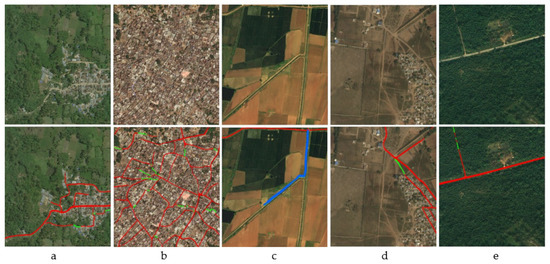
Figure 1.
Uniqueness and difficulty of road extraction based on remote sensing image. The first row is the original test image, and the second row is the prediction output. Red, Green, and Blue indicates TP, FN, and FP (see Section 4.3 for definitions). (a–e) indicates road’s unique and difficult features, which are correspond to the description above (1)~(5).
Recently, various current popular semantic segmentation methods have been published in succession. Fully convolutional networks (FCN) [5] is the first model for Encoder-Decoder supervised learning and pre-training, and it cannot fully capture contextual semantic relationship due to loss of spatial information via using pooling. As a result, researchers proposed efficient multi-scale contextual semantic fusion modules, such as Deeplab’s dilated convolution [6,7,8], pyramid scene parsing network’s (PSPNet’s) pyramid pooling module [9], and encoder-decoder networks for effective fusion of low-level and high-level features at different resolutions, such as U-Net [10], LinkNet [11], and D-LinkNet [3]. In particular, D-LinkNet, as a typical road extraction network, has a good lightweight effect. Of course, there is a shortage of local information loss due to the use of dilated convolution. At present, the emerging attention mechanism [12,13,14] for global information learning has also achieved success in the field of semantic segmentation, such as Non-local [15], PSANet [16], A2Net [17], EMANet [18], and HsgNet [19]. Graph convolution networks (GCN) [20] are also brought into focus because of its strong reasoning learning ability. However, it is still difficult to apply the above method to the extraction task of the complex and occluded roads with features similar to background, especially in the improvement of road connectivity.
Constantly, with the development of location big data, some scholars infer the distribution of road network by tracking the GPS trajectory data of vehicles to extract the road network [21,22,23,24,25]. In [26], researchers used GPS data as input data to improve the road disconnection caused by occlusion, texture similarity, and geometric feature similarity. Apparently, the road connectivity can be improved by introducing multivariate location data, which provides a direction for the re-creation of this paper. However, another problem found in the research process is also worthy of attention and optimization. During the shooting process of remote sensing image, the image distribution will be uneven, and the contrast will be reduced due to the occlusion of cloud and the illumination of light, which therefore leads to the difficulty in pixel classification [27,28,29,30]. Therefore, the enhancement of data pre-processing is another focus of this paper.
In this paper, we aim to increase the accuracy of road extraction and improve the road connectivity via improving the above problems. We propose to improve the performance of hidden representations of the model based on fusion location data, and to improve the road disconnection caused by occlusion, shadow, cloud, etc. We study the general model of the regression method and integrate the data pre-processing and post-processing modules into this paper. In data pre-processing, the histogram equalization [27,31]. is adopted to enhance the remote sensing image data and increase the data contrast and feature difference; in data post-processing, an Iteration Reinforcement (IteR) module is designed to fuse the original information to repeatedly self-correct the prediction output and study the prediction output feature map by Iteration Reinforcement.
The specific contributions of this paper are as follows:
- (1)
- We propose a new road extraction method based on location data fusion and designed a road extraction network based on D-LinkNet, Fusion Network (FuNet) for short. In addition, we studied the general data pre-processing and post-processing methods of the proposed network. We added the Iteration Reinforcement (IteR) module of post-processing function to the output terminal of the network to splice, fuse, and retrain all the information of the original input data and the output results of the network.
- (2)
- We design an IteR module to perform data post-processing. IteR consists of n basic blocks. By introducing multiple iterative optimization techniques, the prediction results can reach an optimal and stable result after multiple optimizations, and the connectivity identification of the road can also be improved when the overall recognition rate of the road model is enhanced. The basic block structure is introduced to improve the performance of the model. The proposed module is universal.
- (3)
- The histogram equalization algorithm is used for data pre-processing of remote sensing image. The data are enhanced by histogram equalization to improve the image contrast. Different from the commonly used data augmentation methods such as image rotation, clipping, and zooming, etc., it makes up for the limited training set caused by the difficulty in semantic segmentation image annotation. The proposed method is universal.
- (4)
- In this paper, we compare and analyze a number of advanced road extraction methods on the public data set BeiJing DataSet [1] to certify the effectiveness and progressiveness of (1)–(3). We also discussed the performance changes of the proposed model under different conditions, including the use of histogram equalization before and after data processing, the role of IteR module, and the changes with the number of basic blocks of the IteR module. According to the discussion results, we gave some feasible suggestions for application in this paper.
This paper is organized as follows: In Section 2, related work is introduced. In Section 3, the proposed methodology based on iteration reinforcement is detailed. The experiment and results are shown in Section 4. The discussion is presented in Section 5. Finally, the conclusion is drawn in Section 6.
2. Related Work
With the rapid development of machine learning and deep learning, some achievements have been accumulated in road extraction. However, it is still difficult to extract road regions based on remote sensing imagery. The research results on road connectivity especially are relatively few.
In the aspect of traditional machine learning, Song and Civco [32] proposed a method to detect road regions using shape index feature and support vector machines (SVM). Das et al. [33] designed a multi-level framework based on two significant road features to extract roads from high-resolution multispectral images using probabilistic SVM. Alshehhi and Marpu [2] presented an unsupervised road extraction method based on hierarchical image segmentation. Recently, a road segmentation result using shallow convolutional neural network combined with multi-feature view-based is published. The network made use of the abstract features extracted from the derived representation of the input image display, and combined gradients information as additional features of the image to obtain better results [34]. These methods rely on prior knowledge and additional features, and the method of deep learning is widely used in road extraction task due to automatically learn features. In the aspect of deep learning, Saito [35] exploited CNN to extract roads directly from the original images and achieved better results in Massachusetts Roads Dataset. RoadTracer [36] proposed by Bastani directly outputted the road network from CNN through the iterative search process based on CNN decision function. Xia et al. [37] also directly used DCNN to extract road and tested them in GF-2 images. According to the newly published research results, some scholars have introduced the idea of deep transfer learning and integrated learning into the extraction task of road target objects in stages to improve the integrity of the roads network [38]. The roads are extracted directly by deep convolutional neural network in the above studies. However, with the continuous progress of deep learning in the field of computer vision, researchers began to do innovative research combined with deep learning. At present, in view of the uniqueness of roads extraction, there are four semantic segmentation techniques based on deep learning are worthy of further study.
The first model that impresses us is the multi-scale and multi-dimensional information fusion network model typically represented by dilated convolution, such as U-Net [10], LinkNet [11], and D-LinkNet [3]. They splice feature maps with different resolutions to integrate low-level detail information and high-level semantic information. In particular, D-LinkNet proposed by Zhou [3] et al. won the first prize in 2018 DeepGlobe Road Extraction Challenge by expanding the receptive field and multi-scale contextual semantic information fusion. However, not all pixels are involved in the calculation due to kernel discontinuity, which results in the loss of spatial information and being unfit for the road extraction that require learning global information.
The second network model is the innovative network based on attention mechanism [12,13,14]. Non-local [15], PSANet [16], OCNet [39], and CCNet [40] models were the first to introduce self-attention in 2018, as well as Local RelationNet [41] model in 2019, which achieved good results in global and long-distance spatial information learning. A2-Nets [17] and CGNL [42] optimized the self-attention mathematically. SGR [43], Beyond Grids [44], GloRe [45], LatentGNN [46], APCNet [47], and EMANet [18] explored and practiced the “low rank” reconstruction. DANet [48] and cross attention network [49] further demonstrated that the attention to the information on the feature channel is conducive to the improvement of semantic segmentation accuracy. Of course, learning global information and long-distance semantics based on attention is effective [50,51], which makes up for the loss of dilated convolution information. However, although attention mechanisms can learn global information, it also brings information redundancy.
The third direction that we are interested in is graph convolution. Graph Convolution Networks (GCN) [20] is a very popular semantic relation reasoning approach for image segmentation in recent years. Different from the CRFs [52] and the random walk network [53,54], GCN is better at learning the global and long-distance spatial information. Wang et al. [55] proposed to use GCN in video recognition task to capture the relation between objects. In the latest invention published by CVPR in 2020, the author exploited the graph convolution to perform semantic sketch segmentation and adopted the graph convolution with two branches to extract intra-stroke and inter-stroke features, respectively [56]. In addition, the popular methods such as GAT [57], GAE [58], and GGN [59] also take GCN as a model to build basic block. However, there are some problems in the above methods. They have not been tested on the task of road extraction, especially on the improvement of road connectivity.
The fourth direction, also one of the issues considered in this paper, is the effective improvement of road connectivity. At first, some scholars exploited the traditional method to improve the road connectivity by using the manually designed finite element model and by combining the contextual prior knowledge, such as High-order CRF [60], Junction-point processes [61], and so on. In recent years, Batra et al. [62] tried to solve the roads topological connectivity by tracking the specific annotation direction in combination with the behavior of manual road annotation. Some researchers generate the road network by smoothing and denoising to GPS data [21,23]. In [26], the combination of remote sensing image and GPS data was input into the model for the first time to improve the road extraction ability of the model. In the road extraction method, we can improve the disconnectivity of the extracted road due to the occlusion of trees, buildings, shadows, and cloud by introducing GPS data.
The performance of semantic segmentation methods above will be better if a data augmentation technique and a data post-processing method can be integrated. The data augmentation technique is still a powerful way to improve the accuracy of semantic segmentation. The effect of traditional data extension methods such as tailoring, rotation, and scaling is not obvious due to the difficulty in annotating data. In particular, due to the low contrast of the acquired remote sensing image data caused by sunlight or weather, the image contrast can be improved by data augmentation, so that the model can identify the target object more easily [27,28,29,30]. Simultaneously, data post-processing is a very common method to improve semantic segmentation, and there are many post-processing methods [62,63]. In [63], a refinement pipeline is introduced to iteratively enhance the prediction output, and the refinement process is performed for the whole model. The predicted segmentation results and the original input images are spliced during the optimization, and then sent to the model for calculation. The approach improves the performance of the model after multiple iterations, but the computation amount is very huge. The refinement method for several iterations is also adopted in [21,22,23,24,25]. Different from the previous method of splicing the prediction results with the original pictures, the prediction results are spliced with the decoded output feature maps, and the model effect is better after multiple iterations. A stacked multi-branch convolutional module is proposed in the model for iteration, instead of the iteration of the entire network, which can effectively utilize the mutual information and reduce the computation amount. Some scholars also employ a post-processing probability layer combined with deep learning to effectively optimize road segmentation [64]. Mnih and Hinton [65] uses RBMs as the basic block to construct the deep neural network and combines pre-processing and post-processing methods further improve the accuracy of road segmentation. The contributions of the above scholars have inspired the research of this paper.
In this paper, we constructed a road extraction network by combining the data pre-processing with histogram equalization and the fusion location data to strengthen the learning of output results by embedding a general IteR module at the end of the network. The IteR module is inspired from [62,63], but the entire network is not iterated to avoid excessive computation; instead, the prediction output is fused with the original image, and the iteration is repeated to achieve self-correction. Experimental results show that the proposed road extraction network of the post-processing module based on IteR and the data pre-processing method are effective. Compared with other experimental methods, the results are optimal, the accuracy of road extraction is increased, and the road connectivity is improved.
3. Methodology
3.1. FuNet Architecture
A novel Fusion Network (FuNet) is proposed to segment remote sensing images, which can be extended to the field of image segmentation. FuNet uses D-LinkNet34 [3] as the main structure for experiments. The network architecture (Figure 2) is connected to the universal Iteration Reinforcement (IteR) after D-LinkNet coding, multi-scale feature fusion, and decoding output, and the original images are fused to conduct auxiliary reinforcement training for output results, so as to further improve the predication output. See Section 3.2 for Iteration Reinforcement (IteR) design.
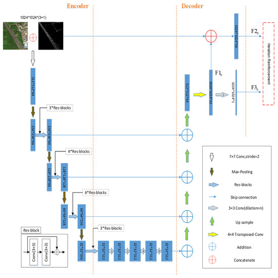
Figure 2.
Fusion network (FuNet) architecture, with D-LinkNet as the backbone network, including coding, multi-scale feature fusion, decoding, and post-processing iteration reinforcement (IteR) module. The blue box is the feature map, and the others are shown in the legend at the lower right corner.
3.2. Iteration Reinforcement
Iteration Reinforcement (Figure 3) is connected to the output terminal of D-LinkNet network to enhance the post-processing of the output data. The input data of D-LinkNet, the deconvolution output of the penultimate layer, and the expansion convolution layer output of the last layer are expressed as , , and . The output of D-LinkNet can be defined as follows:
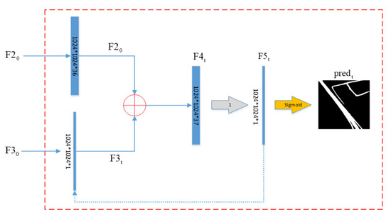
Figure 3.
IteR module. The dotted skip connect indicates that the output feature map of the current basic block will be the input of the next basic block. The blue box is the feature map.
IteR model further integrates multi-dimensional information through repeated iterative enhancement learning of the splicing results of D-LinkNet output data and original images, so that the accuracy of the results will not be affected by information loss when the model is forecasting. The result of splicing with the original input image along the channel is defined as:
is the input of the basic block, which is defined as follows:
is the splicing result of and along the channel in the basic block, which is defined as follows:
is the prediction feature map, which is calculated by the convolution (kernel size is 3, dilation is 1) of , which is defined as follows:
where is the number of basic blocks, which is set to (Section 5.2) after experimental discussion. In Equation (1), and are the output of the penultimate layer and the last layer of D-LinkNet, respectively. In Equations (2) and (4), concat(.) is the splicing along the channel. In Equation (3), is the output feature map of the basic block. In Equation (5), conv(.) is the convolution operation of the input feature map.
When the current basic block is the last one, the predicted is obtained by through the nonlinear transformation layer of sigmoid.
The predicted of each basic block is defined as follows:
If the current basic block is not the last, is passed to of the next basic block along the direction of the dotted arrow, and then Equations (3)–(5) are repeated.
3.3. Loss Function
During the training process of FuNet, each basic block will output the prediction results, and the total loss in the training process will be obtained by calculating the accumulated loss of n basic blocks. Assuming that the basic block outputs the prediction feature map , the prediction result of the current basic block is acquired by through sigmoid layer, and the of and label and the total (Figure 4) are calculated, as defined below:
where is the index of basic block, and is the total number of basic blocks.
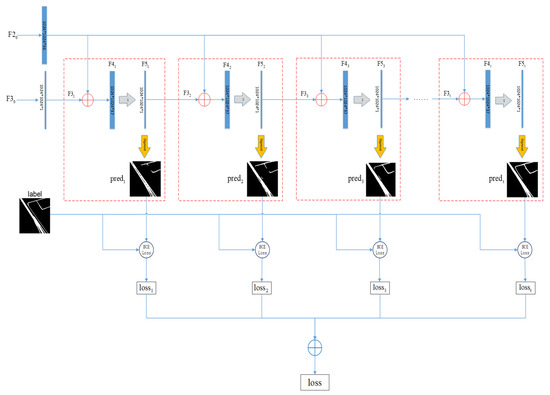
Figure 4.
Loss calculation process in training process.
4. Experiment and Results
4.1. Datasets
The training, verification, and test datasets adopted in this paper are from BeiJing DataSet [1]. Data types include remote sensing (RS) images and global positioning system (GPS) data. The samples of two data sets are shown in Figure 5.
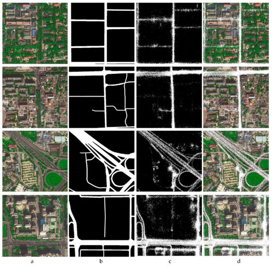
Figure 5.
Data visualization of BeiJing DataSet. (a) Remote sensing image data; (b) label data; (c) global positioning system (GPS) location data (white points); (d) superimposed and fused data.
There are 348 remote sensing images in RS data. Among them, 278 images are used for training verification set, and 70 images are used for testing. Each image has a size of 1024 × 1024 and a pixel resolution of 0.5 m/pixel. The road labels on the image are manually marked by the author. During the training process, the training set and the verification set are randomly divided from the training verification set at 9:1, and the remote sensing image data are randomly enhanced by Scale, Horizontal Flip, Verticle Flip, Rotate 90 degree. We set the random probability to be 0.5. In the training stage, a random number of 0 to 1 is generated for each image. If the random number is less than , then the image will be enhanced; if it is greater than prob, then the image will not be enhanced. Before training, the original remote sensing images are processed by histogram equalization.
GPS data come from 8,100,000 samples taken from 28,000 taxis in Beijing in a week. GPS data in BeiJing DataSet contain latitude, longitude, speed, and sampling interval. The proposed model only uses the latitude and longitude fields of GPS, which can be expressed as . On the basis of spatial position coordinates, we convert GPS points into binary image format according to the corresponding relationship between the original remote sensing image and GPS longitude and latitude. Then, we implement the data fusion by overlaying the GPS binary image and the original remote sensing image in the channel dimension. Results are shown in Figure 5. By comparing them with the original image, we can find that GPS points are concentrated in the trunk road area, while there are GPS points apparently concentrated in some places covered by trees on the remote sensing image. Thus, we can infer whether there is a road through the location and density of GPS points, which is also the fundamental reason for the introduction of location data to improve road connectivity in this paper.
We adopt the index APLS [66] to evaluate connectivity. Then, the labels and prediction results need to be further processed during the testing process. First, the labels and prediction results are extracted from the skeleton line, which is then transformed into a graph structure. On the basis of the graph structure, the road topological connectivity is evaluated by calculating the deviation of the shortest path distance between all node pairs in the label graph and the prediction graph.
4.2. Setup
The network architecture adopted in this paper is based on D-LinkNet and takes advantage of the fusion of multi-dimensional multi-resolution features. See Section 3.1. An iteration reinforcement (IteR) is added at the output end of the network architecture, in which the basic block is , which is an experimental value; please refer to Section 5.2.
The remote sensing image and GPS location data in this paper are from the public BeiJing Dataset [1]. We take Adma as the optimizer [67] and BCE (binary cross entropy) + dice coefficient loss as the loss function [3]. We set the batch size to 16 and the initial learning rate to 1e−4. If the loss of six consecutive epochs verification sets does not drop below the historical minimum value, then the learning rate is multiplied by 0.5. The training is terminated when the training cycle is over 60 epochs, or the learning rate is below 1e−7. During the training, the data are randomly enhanced by Scale, Horizontal Flip, Vertical Flip, Rotate 90 degree. All experiments are tested on a NVIDIA Tesla V100 32G using Ubuntu 18.06 operating system.
4.3. Evolution Metric
The experimental results are evaluated by mean intersection over union (), as defined below:
where is the number of correct samples detected as positive samples, is the number of incorrect samples detected as positive samples, is the number of incorrect samples detected as negative samples, the subscript is the number of samples, and n is the total number of samples.
In addition to the general semantic segmentation index , we take the average path length similarity proposed in [21,66] as another evaluation index to certify that our method can also improve the roads topological connectivity. is an effective index based on graph theory to emphasize the connectivity of the road network. The deviation of the shortest path distance between all node pairs in the graph is captured by the proposed method.
We convert label and prediction output into graph form to get and . The definition of is simply described as follows:
where , . is the total number of nodes in the ground truth graph, is the total number of images, and are the path length between and , respectively. is the cumulative sum of the shortest path difference between all node pairs in the survey graph and the graph . is symmetrically introduced to the calculation of final to punish false positives. is the cumulative sum of the shortest path difference between all node pairs in the survey graph and the graph .
4.4. Results and Analysis
The experimental results of various advanced semantic segmentation methods on BeiJing DataSet [1] are listed in Table 1. We can directly observe that: (1) The accuracy of our model is optimal before and after the fusion of GPS location data. The (63.31%) of the proposed model is 1.38 higher than HsgNet based on attention mechanism and 2.41 higher than D-LinkNet, which was the first place in the road extraction competition in 2018; (2) compared with the model without GPS data, the accuracy of all models with GPS location data is obviously improved; (3) the road connectivity is also effectively improved by the proposed model, but the results are not as good as the Road Connectivity model [62] focusing on road connectivity. These observations can prove that the introducing of location data and data post-processing proposed are effective.

Table 1.
Comparison results after inputting different data. Among them, input data include only remote sensing image data, which is abbreviated to Image; the fusing of GPS and remote sensing image is input, which is abbreviated to GPS+Image.
The visualization results acquired by various methods are shown in Figure 6. From the visualization results, we can clearly see that our model performs best in terms of texture similarity, occlusion, and complex background. In particular, our method also performs well in road connectivity.
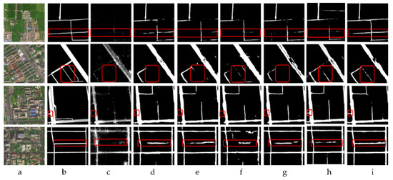
Figure 6.
Visualization results. From left to right: (a) Remote sensing image, (b) label, (c) GPS data, (d) LinkNet, (e) D-LinkNet, (f) road-connectivity, (g) HsgNet, (h) D-LinkNet + 1D, (i) FuNet.
In order to further demonstrate the advantages fusion of GPS location data intuitively, we present the test results of inputting remote sensing image lonely and inputting fusion data of GPS and remote sensing image in Figure 7. We obtained the following observations: (1) Although some roads are occluded by trees or houses, GPS points will be distributed obviously, which indicates the existence of road; (2) when only remote sensing images are used as input data, the blocked road cannot be recognized or effectively identified (column 4); after the fusion of GPS location data, the road segmentation effect is significantly enhanced (column 5). These observation results show that GPS data can improve the recognition and reasoning ability of the model, especially when the road is occluded by trees, houses, shadows, etc., which is also demonstrated in [1,26].
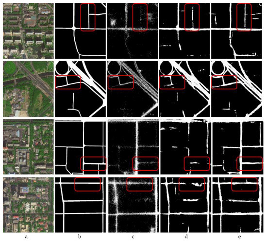
Figure 7.
Comparison results before and after fusing GPS data. (a) Image, (b) label, (c) GPS distribution, (d) the test result of using the original image as the input data alone, (e) the test result of fusing GPS and remote sensing image as the input data.
5. Discussion
5.1. Before vs. After Histogram Equalization
This section aims to further certify the effectiveness and universality of the data pre-processing using histogram equalization. The comparison results before and after using histogram equalization are listed in Table 2. We observe that the accuracy of histogram equalization is generally increased no matter whether the input data is only remote sensing image or fusion data. This observation show that histogram equalization approach can improve the accuracy of road recognition by enhancing the contrast of the image. In high-contrast images, the road region can be separated from the background in a better way to improve the performance of the model in road extraction [27,28,29,30]. However, the comparison with forth column (after HE2) and fifth column (after HE1) experimental results reveal that histogram equalization is required for both the training set and the test set, otherwise the accuracy of road extraction will be reduced. Therefore, in practical application, histogram equalization is available when the contrast of remote sensing image is poor due to shooting, occlusion, illumination, and other factors, but users need to perform image-wise histogram equalization for both training data and application data simultaneously.
Table 2.
The comparison of accuracy (mIoU %) before and after using histogram equalization (HE). The result without using HE is recoded in the third column (before HE). Using HE both in the training set and testing set is recoded in the fourth column (after HE2) and using HE in training set is recoded in the fifth column (after HE1).
To further explain the discussion results above, we present the gray level distribution after histogram equalization of BeiJing DataSet [1] (Figure 8). We can see that before equalization, the foreground and background histograms overlap more at the peak; after equalization, the degree of overlapping decreases, which indicates that the image contrast is enhanced by histogram equalization, and the gray level of the image is adjusted from nonuniform distribution to uniform distribution by gray level transformation. Histogram equalization can be performed for red, green, and blue components of color images. Respectively, to enhance color images. When it is difficult to extract road due to insufficient illumination or serious exposure in aerial images [1], the image contrast is especially improved by histogram equalization.
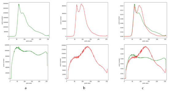
Figure 8.
Histogram comparison before and after histogram equalization. The first row is the histogram distribution of the original image, and the second row is the histogram distribution after histogram equalization. (a) The first column is the background, (b) the second column is the foreground, and (c) the third column is the normalized merge of the foreground and the background.
5.2. Multi Basic Block
This section aims to further certify the effectiveness and generality of IteR module. Before and after histogram equalization, the effect of the number of IteR basic blocks on the model performance is recorded in Table 3. Considering the running time of the model as, without histogram equalization, the optimal result can be achieved when is equal to 5, and the number of IteR modules become 3 while using the histogram equalization (reduced by 2). We observe that the number of IteR modules will reduce after using histogram equalization, which certifies that histogram equalization can improve the model performance.
Table 3.
Statistical results of the changes in the number of IteR basic blocks and the model performance before and after histogram equalization. Statistical items are mIoU (%), time (ms), time relative before and after histogram equalization (HE).
The visualization results of the IteR module () before histogram equalization are shown in Figure 9. We can clearly see that as increases, the model performs better in road extraction. From the second row, we can see that as increases, the non-road objects (red check box) and road objects are identified correctly by the model. The main reason for this phenomenon is similar to self-correcting principle described in [68]. We fuse the output data and the original image information by repeated IteR to prevent the low-level information loss. The effectiveness of the proposed method has also been certified in previous studies [21,22,23,24,25].
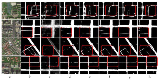
Figure 9.
Visual display of road segmentation using different number of basic blocks. n denotes the number basic blocks, . (a) The original image, (b) label data, (c) GPS location data, and (d) , (e) , (f) , (g) , (h) , where is the number of IteR basic blocks.
We discussed the effect of the number of basic blocks in IteR model on the accuracy of results before and after histogram equalization, respectively. As can be seen from Table 3 and Figure 10: (1) As the number of basic blocks increases, the accuracy of the model is improved and then declines and tends to be stable; (2) as the number of basic blocks n increases, the running time of the model increases continuously; (3) the size of the model will not increase significantly with the change of , regardless of whether the data pre-processing with histogram equalization is used; (4) without the histogram equalization, the accuracy of the model is optimal when is equal to 7. However, considering both the running time and accuracy of the model, it is more appropriate for to be 5; with histogram equalization, the optimal accuracy of the model is achieved when is 3. By further processing and calculation, we can conclude that: (1) No matter whether using the histogram equalization, the test time increases by about 1.7 ms when n increases by 1; (2) when n is equal, the running time with histogram equalization is 3.4 ms longer than that without histogram equalization. However, the number of IteR basic blocks can be reduced by the histogram equalization. Further comparison shows that: (1) The predictive ability of the model without histogram equalization is positively correlated with increasing when is less than 5, and the predictive ability declines and tends to be stable when is greater than 7; after histogram equalization, the peak occurs when is equal to 3, and the number of basic blocks decreases; (2) when the number of IteR basic blocks without histogram equalization is 5, the optimal is 63.31%, and the running time is 42.30ms; when the number of IteR basic blocks with histogram equalization is 3, the maximum is 63.36%, and the running time is 42.54 ms. These data guide us how to select before and after using histogram equalization.
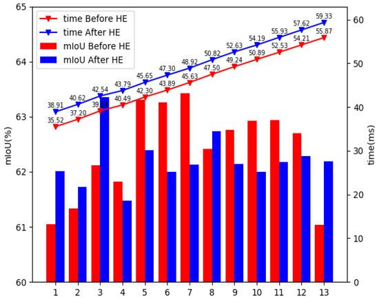
Figure 10.
Relationship between model performance and IteR basic block number .
To sum up, the number of IteR modules can be reduced by the data pre-processing with histogram equalization in the case of guaranteeing accuracy and efficiency, so according to the quality of remote sensing image, n is equal to 5 without histogram equalization; n is equal to 3 with histogram equalization. Finally, it is recommended to employ both data pre-processing with histogram equalization and IteR data post-processing in practice application.
6. Conclusions
This paper mainly aims to improve the accuracy of road extraction and the road connectivity. The innovative achievements in this paper are as follows: We (1) proposed a novel Fusion Network (FuNet) to integrate remote sensing image data and location data and enhance the learning performance of the network; (2) designed an universal Iteration Reinforcement (IteR) model to self-correct and optimize the model by fusing the prediction output and original image information and to enhance the network learning ability; designed an reinforcement loss function to improve the accuracy of road prediction label; and (3) exploited the data pre-processing with histogram equalization to improve the image contrast with better effect, which is increased by nearly 1%. The data pre-processing method is also universal. We also designed experiments with D-LinkNet as the backbone network structure and compared several advanced road extraction methods in BeiJing DataSet. This paper focuses on the data pre-processing and post-processing, analyzes, and discusses the performance of the histogram equalization and the number of basic blocks in IteR module, and gives practical application suggestions. Experimental results show that our model performs best, which improves the accuracy of road extraction and the road topological connectivity. To sum up, according to Section 5, we suggest to use both data post-processing based on IteR and data pre-processing based on histogram equalization, but users need to perform image-wise histogram equalization for both training data and application data simultaneously.
In future work, we will continue to study the complex road extraction from satellite images, which is a necessary and important research topic. We plan to adopt the way of multi-source data fusion, especially to give full play to the auxiliary advantage of the location big data, and further improve the accuracy of road extraction by introducing the multi-source information fusion such as direction and spatial relationship of road.
Author Contributions
Conceptualization, Kai Zhou and Yan Xie; methodology, Yan Xie and Kai Zhou; software, Lei Zhang and Yan Xie; validation, Lei Zhang and Yan Xie; formal analysis, Kai Zhou, Zhan Gao, and Fang Miao; investigation, Kai Zhou and Yan Xie; resources, Kai Zhou and Zhan Gao; data curation, Kai Zhou; writing—original draft preparation, Yan Xie, Kai Zhou, and Lei Zhang; writing—review and editing, Yan Xie, Kai Zhou, Lei Zhang, Zhan Gao, and Fang Miao; visualization, Lei Zhang and Yan Xie; supervision, Zhan Gao and Fang Miao; project administration, Kai Zhou and Yan Xie; funding acquisition, Kai Zhou. All authors have read and agreed to the published version of the manuscript.
Funding
This research was funded by the key research and development task of Sichuan science and technology planning project (2019YFS0067), Research and application of the key techniques of regional dynamic extraction and visual change monitoring of Tibetan remote sensing image in Sichuan province (2020YFS0364).
Acknowledgments
The authors would like to thank the company of Da Cheng Jun Tu for the supporting computing environment. Meanwhile, we thank the editors and reviewers for their valuable comments.
Conflicts of Interest
The authors declare no conflict of interest.
References
- Sun, T.; Di, Z.; Che, P.; Liu, C.; Wang, Y. Leveraging Crowdsourced GPS Data for Road Extraction from Aerial Imagery. In Proceedings of the 2019 IEEE/CVF Conference on Computer Vision and Pattern Recognition (CVPR), Long Beach, CA, USA, 15–20 June 2019; pp. 16–20. [Google Scholar]
- Alshehhi, R.; Marpu, P.R. Hierarchical graph-based segmentation for extracting road networks from high-resolution satellite images. ISPRS J. Photogramm. Remote Sens. 2017, 126, 245–260. [Google Scholar] [CrossRef]
- Zhou, L.; Zhang, C.; Wu, M. D-LinkNet: LinkNet with Pretrained Encoder and Dilated Convolution for High Resolution Satellite Imagery Road Extraction. In Proceedings of the 2018 IEEE/CVF Conference on Computer Vision and Pattern Recognition Workshops (CVPRW), Salt Lake City, UT, USA, 18–22 June 2018; pp. 192–1924. [Google Scholar]
- Zhang, Z.; Liu, Q.; Wang, Y. Road Extraction by Deep Residual U-Net. IEEE Geosci. Remote Sens. Lett. 2018, 15, 749–753. [Google Scholar] [CrossRef]
- Shelhamer, E.; Long, J.; Darrell, T. Fully Convolutional Networks for Semantic Segmentation. arXiv 2016, arXiv:1411.4038. [Google Scholar] [CrossRef]
- Chen, L.-C.; Papandreou, G.; Kokkinos, I.; Murphy, K.; Yuille, A.L. DeepLab: Semantic Image Segmentation with Deep Convolutional Nets, Atrous Convolution, and Fully Connected CRFs. arXiv 2016, arXiv:1606.00915. [Google Scholar] [CrossRef] [PubMed]
- Chen, L.-C.; Papandreou, G.; Schroff, F.; Adam, H. Rethinking Atrous Convolution for Semantic Image Segmentation. arXiv 2017, arXiv:1706.05587. [Google Scholar]
- Chen, L.-C.; Zhu, Y.; Papandreou, G.; Schroff, F.; Adam, H. Encoder-Decoder with Atrous Separable Convolution for Semantic Image Segmentation. arXiv 2018, arXiv:1802.02611. [Google Scholar]
- Zhao, H.; Shi, J.; Qi, X.; Wang, X.; Jia, J. Pyramid Scene Parsing Network. arXiv 2016, arXiv:1612.01105. [Google Scholar]
- Ronneberger, O.; Fischer, P.; Brox, T. U-Net: Convolutional Networks for Biomedical Image Segmentation. arXiv 2015, arXiv:1505.04597. [Google Scholar]
- Chaurasia, A.; Culurciello, E. LinkNet: Exploiting Encoder Representations for Efficient Semantic Segmentation. In Proceedings of the 2017 IEEE Visual Communications and Image Processing (VCIP), St. Petersburg, FL, USA, 10–13 December 2017; pp. 1–4. [Google Scholar]
- Vaswani, A.; Shazeer, N.; Parmar, N.; Uszkoreit, J.; Jones, L.; Gomez, A.N.; Kaiser, L.; Polosukhin, I. Attention Is All You Need. arXiv 2017, arXiv:1706.03762. [Google Scholar]
- Jaderberg, M.; Simonyan, K.; Zisserman, A. Spatial Transformer Networks. Adv. Neural Inf. Process. Syst. 2015, 28, 2017–2025. [Google Scholar]
- Wang, F.; Jiang, M.; Qian, C.; Yang, S.; Li, C.; Zhang, H.; Wang, X.; Tang, X. Residual Attention Network for Image Classification. arXiv 2017, arXiv:1704.06904. [Google Scholar]
- Wang, X.; Girshick, R.; Gupta, A.; He, K. Non-local Neural Networks. In Proceedings of the 2018 IEEE/CVF Conference on Computer Vision and Pattern Recognition, Salt Lake City, UT, USA, 18–22 June 2018; pp. 7794–7803. [Google Scholar]
- Zhao, H.; Zhang, Y.; Liu, S.; Shi, J.; Loy, C.C.; Lin, D.; Jia, J. PSANet: Point-wise Spatial Attention Network for Scene Parsing. In Computer Vision—ECCV 2018; Ferrari, V., Hebert, M., Sminchisescu, C., Weiss, Y., Eds.; Springer International Publishing: Cham, Switzerland, 2018; Volume 11213, pp. 270–286. ISBN 978-3-030-01239-7. [Google Scholar]
- Chen, Y.; Kalantidis, Y.; Li, J.; Yan, S.; Feng, J. A^2-Nets: Double Attention Networks. In Advances in Neural Information Processing Systems 31; Bengio, S., Wallach, H., Larochelle, H., Grauman, K., Cesa-Bianchi, N., Garnett, R., Eds.; Curran Associates, Inc.: Red Hook, NY, USA, 2018; pp. 352–361. [Google Scholar]
- Li, X.; Zhong, Z.; Wu, J.; Yang, Y.; Lin, Z.; Liu, H. Expectation-Maximization Attention Networks for Semantic Segmentation. arXiv 2019, arXiv:1907.13426. [Google Scholar]
- Xie, Y.; Miao, F.; Zhou, K.; Peng, J. HsgNet: A Road Extraction Network Based on Global Perception of High-Order Spatial Information. ISPRS Int. J. Geo.-Inf. 2019, 8, 571. [Google Scholar] [CrossRef]
- Kipf, T.N.; Welling, M. Semi-Supervised Classification with Graph Convolutional Networks. arXiv 2017, arXiv:1609.02907. [Google Scholar]
- Biagioni, J.; Eriksson, J. Map inference in the face of noise and disparity. In Proceedings of the 20th International Conference on Advances in Geographic Information Systems; Association for Computing Machinery: New York, NY, USA, 2012; pp. 79–88. [Google Scholar]
- Karagiorgou, S.; Pfoser, D.; Skoutas, D. A Layered Approach for More Robust Generation of Road Network Maps from Vehicle Tracking Data. ACM Trans. Spat. Algorithms Syst. 2017. [Google Scholar] [CrossRef]
- Liu, X.; Biagioni, J.; Eriksson, J.; Wang, Y.; Forman, G.; Zhu, Y. Mining large-scale, sparse GPS traces for map inference: Comparison of approaches. In Proceedings of the 18th ACM SIGKDD International Conference on Knowledge Discovery and Data Mining; Association for Computing Machinery: New York, NY, USA, 2012; pp. 669–677. [Google Scholar]
- Shan, Z.; Wu, H.; Sun, W.; Zheng, B. COBWEB: A robust map update system using GPS trajectories. In Proceedings of the 2015 ACM International Joint Conference on Pervasive and Ubiquitous Computing, Osaka, Japan, 7–11 September 2015; pp. 927–937. [Google Scholar]
- Wang, Y.; Liu, X.; Wei, H.; Forman, G.; Zhu, Y. CrowdAtlas: Self-updating maps for cloud and personal use. In Proceedings of the 11th Annual International Conference on Mobile Systems, Applications, and Services, Taipei, Taiwan, 25–28 June 2013; pp. 469–470. [Google Scholar]
- Sun, T.; Di, Z.; Che, P.; Liu, C.; Wang, Y. Leveraging Crowdsourced GPS Data for Road Extraction from Aerial Imagery. arXiv 2019, arXiv:1905.01447. [Google Scholar]
- Al-Sammaraie, M.F. Contrast enhancement of roads images with foggy scenes based on histogram equalization. In Proceedings of the 2015 10th International Conference on Computer Science Education (ICCSE), Cambridge, UK, 22–24 July 2015; pp. 95–101. [Google Scholar]
- Shadeed, W.G.; Abu-Al-Nadi, D.I.; Mismar, M.J. Road traffic sign detection in color images. In Proceedings of the 10th IEEE International Conference on Electronics, Circuits and Systems, Sharjah, United Arab Emirates, 14–17 December 2003; Volume 2, pp. 890–893. [Google Scholar]
- Fernández Caballero, A.; Maldonado Bascón, S.; Acevedo Rodríguez, J.; Lafuente Arroyo, S.; López Ferreras, F. An optimization on pictogram identification for the road-sign recognition task using svms. Comput. Vis. Image Underst. 2010, 114, 373–383. [Google Scholar]
- Onyedinma, E.; Onyenwe, I.; Inyiama, H. Performance Evaluation of Histogram Equalization and Fuzzy image Enhancement Techniques on Low Contrast Images. Int. J. Comput. Sci. Softw. Eng. 2019, 8, 144–150. [Google Scholar]
- Gonzalez, R.C.; Woods, R.E. Digital Image Processing; Addison-Wesley: Boston, MA, USA, 1977. [Google Scholar]
- Song, M.; Civco, D. Road Extraction Using SVM and Image Segmentation. Photogramm. Eng. Remote Sens. 2004, 70, 1365–1371. [Google Scholar] [CrossRef]
- Das, S.; Mirnalinee, T.T.; Varghese, K. Use of Salient Features for the Design of a Multistage Framework to Extract Roads from High-Resolution Multispectral Satellite Images. IEEE Trans. Geosci. Remote Sens. 2011, 49, 3906–3931. [Google Scholar] [CrossRef]
- Junaid, M.; Ghafoor, M.; Hassan, A.; Khalid, S.; Tariq, S.A.; Ahmed, G.; Zia, T. Multi-Feature View-Based Shallow Convolutional Neural Network for Road Segmentation. IEEE Access 2020, 8, 36612–36623. [Google Scholar] [CrossRef]
- Saito, S.; Yamashita, T.; Aoki, Y. Multiple Object Extraction from Aerial Imagery with Convolutional Neural Networks. J. Imaging Sci. Technol. 2016, 60, 104021–104029. [Google Scholar] [CrossRef]
- Bastani, F.; He, S.; Abbar, S.; Alizadeh, M.; Balakrishnan, H.; Chawla, S.; Madden, S.; DeWitt, D. RoadTracer: Automatic Extraction of Road Networks from Aerial Images. In Proceedings of the 2018 IEEE/CVF Conference on Computer Vision and Pattern Recognition, Salt Lake City, UT, USA, 18–22 June 2018; pp. 4720–4728. [Google Scholar]
- Xia, W.; Zhang, Y.-Z.; Liu, J.; Luo, L.; Yang, K. Road Extraction from High Resolution Image with Deep Convolution Network—A Case Study of GF-2 Image. Proceedings 2018, 2, 325. [Google Scholar] [CrossRef]
- Senthilnath, J.; Varia, N.; Dokania, A.; Anand, G.; Benediktsson, J.A. Deep TEC: Deep Transfer Learning with Ensemble Classifier for Road Extraction from UAV Imagery. Remote Sens. 2020, 12, 245. [Google Scholar] [CrossRef]
- Yuan, Y.; Wang, J. OCNet: Object Context Network for Scene Parsing. arXiv 2018, arXiv:1809.00916. [Google Scholar]
- Huang, Z.; Wang, X.; Huang, L.; Huang, C.; Wei, Y.; Liu, W. CCNet: Criss-Cross Attention for Semantic Segmentation. arXiv 2018, arXiv:1811.11721. [Google Scholar]
- Hu, H.; Zhang, Z.; Xie, Z.; Lin, S. Local Relation Networks for Image Recognition. arXiv 2019, arXiv:1904.11491. [Google Scholar]
- Yue, K.; Sun, M.; Yuan, Y.; Zhou, F.; Ding, E.; Xu, F. Compact Generalized Non-local Network. arXiv 2018, arXiv:1810.13125. [Google Scholar]
- Liang, X. Symbolic Graph Reasoning Meets Convolutions. In Proceedings of the 32nd International Conference on Neural Information Processing Systems; Curran Associates Inc.: Red Hook, NY, USA, 2018; p. 11. [Google Scholar]
- Li, Y.; Gupta, A. Beyond Grids: Learning Graph Representations for Visual Recognition. In Proceedings of the (NeurIPS) Neural Information Processing Systems, Montreal, QC, Canada, 3–8 December 2018; p. 11. [Google Scholar]
- Chen, Y.; Rohrbach, M.; Yan, Z.; Shuicheng, Y.; Feng, J.; Kalantidis, Y. Graph-Based Global Reasoning Networks. arXiv 2018, arXiv:1811.12814. [Google Scholar]
- Zhang, S.; Yan, S.; He, X. LatentGNN: Learning Efficient Non-local Relations for Visual Recognition. arXiv 2019, arXiv:1905.11634. [Google Scholar]
- He, J.; Deng, Z.Y.; Zhou, L.; Wang, Y.; Qiao, Y. Adaptive Pyramid Context Network for Semantic Segmentation. In Proceedings of the 2019 IEEE/CVF Conference on Computer Vision and Pattern Recognition (CVPR), Long Beach, CA, USA, 15–20 June 2019; pp. 7511–7520. [Google Scholar]
- Fu, J.; Liu, J.; Tian, H.; Li, Y.; Bao, Y.; Fang, Z.; Lu, H. Dual Attention Network for Scene Segmentation. arXiv 2018, arXiv:1809.02983. [Google Scholar]
- Liu, M.; Yin, H. Cross Attention Network for Semantic Segmentation. arXiv 2019, arXiv:1907.10958. [Google Scholar]
- Zhu, Q.; Zhong, Y.; Liu, Y.; Zhang, L.; Li, D. A Deep-Local-Global Feature Fusion Framework for High Spatial Resolution Imagery Scene Classification. Remote Sens. 2018, 10, 568. [Google Scholar]
- Xu, Y.; Xie, Z.; Feng, Y.; Chen, Z. Road Extraction from High-Resolution Remote Sensing Imagery Using Deep Learning. Remote Sens. 2018, 10, 1461. [Google Scholar] [CrossRef]
- Lafferty, J.; Mccallum, A.; Pereira, F. Conditional Random Fields: Probabilistic Models for Segmenting and Labeling Sequence Data. In Proceedings of the Eighteenth International Conference on Machine Learning, Williamstown, MA, USA, 28 June–1 July 2001; pp. 282–289. [Google Scholar]
- Lao, N.; Mitchell, T.; Cohen, W.W. Random Walk Inference and Learning in a Large Scale Knowledge Base. In Proceedings of the 2011 Conference on Empirical Methods in Natural Language Processing; Association for Computational Linguistics: Edinburgh, UK, 2011; pp. 529–539. [Google Scholar]
- Bertasius, G.; Torresani, L.; Yu, S.X.; Shi, J. Convolutional Random Walk Networks for Semantic Image Segmentation. arXiv 2017, arXiv:1605.07681. [Google Scholar]
- Wang, X.; Gupta, A. Videos as Space-Time Region Graphs. In Proceedings of the Computer Vision—ECCV 2018; Ferrari, V., Hebert, M., Sminchisescu, C., Weiss, Y., Eds.; Springer International Publishing: Cham, Switzerland, 2018; pp. 413–431. [Google Scholar]
- Yang, L.; Zhuang, J.; Fu, H.; Zhou, K.; Zheng, Y. SketchGCN: Semantic Sketch Segmentation with Graph Convolutional Networks. arXiv 2020, arXiv:2003.00678. [Google Scholar]
- Veličković, P.; Cucurull, G.; Casanova, A.; Romero, A.; Liò, P.; Bengio, Y. Graph Attention Networks. arXiv 2018, arXiv:1710.10903. [Google Scholar]
- Kipf, T.N.; Welling, M. Variational Graph Auto-Encoders. arXiv 2016, arXiv:1611.07308. [Google Scholar]
- Li, Y.; Tarlow, D.; Brockschmidt, M.; Zemel, R. Gated Graph Sequence Neural Networks. arXiv 2017, arXiv:1511.05493. [Google Scholar]
- Wegner, J.D.; Montoya-Zegarra, J.A.; Schindler, K. A Higher-Order CRF Model for Road Network Extraction. In Proceedings of the 2013 IEEE Conference on Computer Vision and Pattern Recognition, Portland, OR, USA, 23–28 June 2013; pp. 1698–1705. [Google Scholar]
- Chai, D.; Forstner, W.; Lafarge, F. Recovering Line-Networks in Images by Junction-Point Processes. In Proceedings of the 2013 IEEE Conference on Computer Vision and Pattern Recognition, Portland, OR, USA, 23–28 June 2013; pp. 1894–1901. [Google Scholar]
- Batra, A.; Singh, S.; Pang, G.; Basu, S.; Jawahar, C.V.; Paluri, M. Improved Road Connectivity by Joint Learning of Orientation and Segmentation. In Proceedings of the IEEE Conference on Computer Vision and Pattern Recognition, Long Beach, CA, USA, 15–21 June 2019; p. 9. [Google Scholar]
- Mosinska, A.; Marquez-Neila, P.; Kozinski, M.; Fua, P. Beyond the Pixel-Wise Loss for Topology-Aware Delineation. In Proceedings of the IEEE Conference on Computer Vision and Pattern Recognition, Salt Lake City, UT, USA, 18–22 June 2018; pp. 3136–3145. [Google Scholar]
- Chen, W. Road Segmentation based on Deep Learning with Post-Processing Probability Layer. In Proceedings of the 6th International Conference on Mechatronics and Mechanical Engineering, Wuhan, China, 9–11 November 2019; Volume 719, p. 012076. [Google Scholar]
- Mnih, V. Machine Learning for Aerial Image Labeling. Ph.D. Thesis, University of Toronto, Toronto, ON, Canada, 2013. [Google Scholar]
- Van Etten, A.; Lindenbaum, D.; Bacastow, T.M. SpaceNet: A Remote Sensing Dataset and Challenge Series. arXiv 2018, arXiv:1807.01232. [Google Scholar]
- Kingma, D.P.; Lei, J. Adam: A Method for Stochastic Optimization. arXiv 2015, arXiv:1412.6980. [Google Scholar]
- Ibrahim, M.S.; Vahdat, A.; Ranjbar, M.; Macready, W.G. Semi-Supervised Semantic Image Segmentation with Self-correcting Networks. arXiv 2020, arXiv:1811.07073. [Google Scholar]


Publisher’s Note: MDPI stays neutral with regard to jurisdictional claims in published maps and institutional affiliations. |
© 2021 by the authors. Licensee MDPI, Basel, Switzerland. This article is an open access article distributed under the terms and conditions of the Creative Commons Attribution (CC BY) license (http://creativecommons.org/licenses/by/4.0/).