Radio Base Stations and Electromagnetic Fields: GIS Applications and Models for Identifying Possible Risk Factors and Areas Exposed. Some Exemplifications in Rome

Abstract

This paper—which is contextualized in the discussion on the methodological pluralism and the main topics of medical geography, the complexity theory in geographies of health, the remaking of medical geography and ad hoc systems of data elaboration—focuses on radio base stations (RBSs) as sources of electromagnetic fields, to provide GIS applications and simplifying-prudential models that are able to identify areas that could potentially be exposed to hazard. After highlighting some specific aspects regarding RBSs and their characteristics and summarizing the results of a number of studies concerning the possible effects of electromagnetic fields on health, we have taken an area of north-east Rome with a high population and building density as a case study, and we have provided some methodological and applicative exemplifications for different situations and types of antennas. Through specific functionalities and criteria, drawing inspiration from a precautionary principle, these exemplifications show some particular cases in order to support: possible risk factor identification, surveillance and spatial analysis; correlation analysis between potential risk factors and outbreak of diseases and symptoms; measurement campaigns in heavily exposed areas and buildings; education policies and prevention actions. From an operative viewpoint, we have: conducted some field surveys and recorded data and images with specific geotechnological and geomatics instruments; retraced the routes by geobrowsers and basemaps and harmonized and joined up the materials in a GIS environment; used different functions to define, on aero-satellite images, concentric circular buffer zones starting from each RBS, and geographically and geometrically delimited the connected areas subject to high and different exposure levels; produced digital applications and tested prime three-dimensional models, in addition to a video from a bird’s eye view perspective, able to show the buildings in the different buffer zones and which are subject to a hazard hierarchy due to exposure to an RBS. A similar GIS-based model—reproposable with methodological adjustments to other polluting sources—can make it possible to conceive a dynamic and multiscale digital system functional in terms of strategic planning, decision-making and public health promotion in a performant digital health information system.

1. Introduction and Contextualization

This paper addresses some of the objectives of medical geography among which are those of analyzing and recognizing [1] (pp. 45–48), [2] (pp. 84–87): the risk factors localized and widespread over the territory; the direct relation between certain risk factors and the outbreak of connected diseases; the correlation between environmental (and behavioral) factors and pathologies; the distribution of diseases and the causes of the distributions; the areas subject to specific diseases and complication due to the presence of health status determinants and zones that differ from such patterns. A notable relevance is thus acquired from the interaction between anthropic components and different environments at various geographical scales, which can be considered as “mutually interacting forces” [3] (p. 1); the social environment can strongly influence both the diffusion of communicable and noncommunicable diseases with increasingly complex and varied modes, the spread of new diseases and the reinforcement of some degenerative forms.

Thus, the present work intersects from an applicative viewpoint with the discussions regarding:

• the methodological pluralism of medical geography which, i.e., involves historical evolution and dynamics, quantitative and qualitative methods, computer mapping, GIS and geospatial analysis [4] (p. 1), with a view to digitally investigating and representing trends, patterns and clusters in a geotechnological environment;
• the main topics of medical geography, through the advancement of new research methods and elaborations, the engagement with real world social issues and problems, the development of innovative approaches which are also due to highly collaborative and interdisciplinary perspectives [5] (pp. 198–199);
• the complexity theory in geographies of health, with entrenched areas of study—which can be highly productive—and new themes and directions [6];
• the remaking of medical geography, which has to consider multiple and updated theories, methodologies, instruments and phenomena in order to actively contribute to social utility, public policy at different geographic scales, global interest in creating awareness and seeking new ways of understanding [7] (p. 17);
• sanitary data collection and statistical methods of data elaboration [8], arriving at spatial analysis and spatial statistics, in a GIS environment, for investigating health data and the associations between exposure and disease risk [9], in order to “support spatial decision-making in public health through applying the evolving analytical approaches to dealing with healthcare planning issues” [10] (p. 1).

The influence of social-economic and cultural-political contexts and the behavioral approach emerges, above all, in the urban environments, where the spatial model of diseases and risk factors are widely influenced by artificial components undergoing rapid evolution [11] (p. 17). Therefore, it is important to move toward a spatial understanding of a community’s health, a screening of the distribution of disease and pollution or transmission source in an area, and an evaluation of the effects on health produced by the environment in a broad sense [12] (p. 1). In light of the complex transformation in the urban contexts—and, at present, the enormous request for high quality IT (Information Technology) and diffused services—it becomes fundamental to consider the variations in health status and health policies [13] (p. 565), which should guarantee suitable levels of public (and individual) safety. Thus, from these perspectives, GIS modeling in health studies takes on a relevant role in order to [14] (p. 15): understand changes in environmental hazards and identify pollution sources which could be mitigated after recognizing hotspot exposure; evaluate variations in population distribution, density and characteristics, including morbidity and susceptibility; address policies and measures that can benefit from a geographically targeted analysis. Moreover, a similar applied approach—based on GIS elaborations and geospatial, multitemporal and geostatistical investigations—can be useful to predict where a high incidence of a specific disease could occur or resurface [15] (p. 1).

The possibility to model the presence and distribution of known or potential risk factors is important to promote and plan health intervention measures and activities after notifying people living near identified hazards, in order to prevent associated health problems; so, investigating how the characteristics and local factors of places interact with the health of communities becomes critically useful for supporting geographically based public health guidelines [16] (pp. 6, 10). Spatial data and models and local estimates of spatial clustering and concentrations, three-dimensional representations and effective digital visualization become vital, driving applicative components for recognizing factors (probably) associated with the distribution of certain symptoms and diseases and for understanding the reasons for which, in some areas, a seemingly anomalous amount of pathologies are recorded [17]. With the aim of addressing these needs, the early identification of the possible risks for the people exposed, rapid methods and analysis are needed to promote ad hoc measures and to investigate potentially increased disease hazards around specific and often widely diffused point sources [18] (p. 255).

Sometimes, as in the case of radio base stations (RBSs) and related electromagnetic fields, we find ourselves faced with point sources, where it is easy to distinguish the source of discharge and pollution, but we are also faced with nonpoint sources, because many widely diffused elements contribute to affecting and exposing people and buildings in different directions; therefore, from a medical geography and public health viewpoint, it is essential to recognize possible risk factors before exposure can produce tangible adverse effects on human health [16] (pp. 187, 188). In fact, many technological innovations have spread without evaluating the possible repercussions and impacts on human and environmental health in advance; a late discovery of a useful and widely and strongly appreciated product or service being damaging to health is often not followed by a reduction in its use [19] (p. 3), refusal of a similar finding or thinking that it is by now a diffused product or service; everyone uses it, which is consequently useless to deny. It is a passive behavior which leads to inaction and apathetic remissibility in terms acquired habits, homogenization of thought and a wish to continue to enjoy a specific service which seems essential, but sometimes the reason for a similar attitude is the absence of deep knowledge of the potential negative effects of certain exposures or substances [20] (p. 472).

In particular, in order to address these issues, in the present work we have combined different methods and instruments related to field surveys, devices for glocalization and measurement, GIS elaborations, spatial analysis and specific functions, three-dimensional modeling and videos.

On the basis of these assumptions, we have focused our attention on supposed risk factors for exemplifying applications, on electromagnetic fields and specifically on possible radio base stations which receive and transmit mobile phone signals which are widely used and particularly concentrated in high population density areas or in those with special needs (universities, hospitals, commercial areas and centers, rail stations, etc.). Generally, each RBS serves a specific surface and the territory is conventionally divided into hexagonal cells of competence [21] (pp. 3–5), (https://www.arpae.it/dettaglio_generale.asp?id=78&idlivello=189)—according to a typical shape for geographical studies and models, without empty space—of varying size and on the basis of: population density and subscribers using the service; power and type of antenna; height of constructions and surrounding buildings and presence of possible structural obstacles for the transmission. In urban areas, there is a considerable number of radio base stations, situated at different heights, on the roof of buildings or on apposite trellises, and with different characteristics, in order to support telecommunications and technological development. However, radio base stations are tendentially present also in small municipalities attempting to reduce the digital divide and satisfy the needs of residents and tourists.

In terms of risk factors, the radio base stations and electromagnetic fields acquire particular relevance because the actual trends make it possible to think about further fast developments, since there is a spasmodic quest (also by children and young people) to increase and upgrade connection capacity and speed.

Moreover, the WHO/International Agency for Research on Cancer (IARC) classified radiofrequency electromagnetic fields as possibly carcinogenic in humans (Group 2B), underlining the importance of other specific and in-depth studies (2011) [22], as also explained in a synthetic and connected work about carcinogenicity of radiofrequency electromagnetic fields [23]. Wide-ranging research and discussion is available in the volume Non-Ionizing Radiation, Part 2: Radiofrequency Electromagnetic Fields [24], where human exposure to radiofrequency electromagnetic fields is investigated and analyzed according to the use of personal devices (e.g., mobile telephones, cordless phones and Bluetooth) and from environmental sources (e.g., mobile-phone base stations, broadcast antennae, etc.), in addition to occupational sources (e.g., high-frequency dielectric and induction heaters and high-powered pulsed radars).

Thus, for this case study, we considered an area of north-east Rome (Lazio region, Italy) characterized by a high population and building density, where many different radio base stations are located to make it possible to have a wide and satisfactory network coverage. In this work, some elaborations are shown considering different types of (probable) RBSs, sometimes with the phenomenon of cositing (i.e., the same construction is shared by more than one operator), which have a notable visual impact and therefore often cause anxiety and worries in the exposed population.

The main aim of this paper is to provide and test exemplificative applicative models in a GIS environment—by drawing inspiration from a precautionary principle—to highlight the presence of potential risk factors, with reference to radio base stations and electromagnetic fields, and geographically and geometrically delimit the connected areas subject to the highest and different exposure levels. Through specific functionalities, concentric buffer zones and prime three-dimensional models, we show some particular cases which act as pilot applications for repetitions on a vast radius and on the whole coverage in the municipality’s territory in order to support:

• further GIS elaborations and geotechnological methods strictly related to sanitary and epidemiological studies;
• correlation analysis between supposed risk factors and outbreak of diseases and symptoms;
• measurement campaigns in heavily exposed areas and buildings;
• awareness and education policies and prevention actions.

2. A General Framework

In Italy, a rapid increase in the number of radio base stations has been an recorded since 2002, after Legislative Decree No. 198, of 4 September 2002 (article 1), which has the following among its goals (https://www.gazzettaufficiale.it/eli/id/2002/09/13/002G0228/sg):

• to facilitate the liberalization of the telecommunications sector, allowing all operators to promptly build their own infrastructures, thus creating a truly competitive market;
• to allow the construction of new generation infrastructures and the adaptation of pre-existing ones to meet the demands linked to technological development;
• to ensure that the construction of telecommunications infrastructures is coherent with the protection of the environment and public health in terms of the limits of exposure, attention values and quality objectives, relative to electromagnetic emissions as referred to in Act No. 36, of 22 February 2001, and related implementation measures;
• to ensure the conditions that will allow the operators to offer innovative services to citizens and users, under a free market regime, thus promoting the pursuit of quality objectives by the sector operators;
• to promote an adequate diffusion of telecommunication infrastructures across the whole national territory.

Therefore, antennas of different types and dimensions have become widespread over the Italian territory to support the development of telecommunications and an efficient and fast reception of mobile phones and instruments (tablet, notebook, GPS, etc.), but at the same time they have brought about an increase in the related radiation emissions, with possible impacts on the emotive and health status of the population residing in the vicinity of the RBS.

Thus, there may often be a tendency to pass from a stage of general and generic perception, experienced with superficiality, to a stage of strong individual psychic perception, which can sometimes become traumatic and involve the family sphere, leading to an alteration in daily tranquility and rituality [25] (p. 375). The intersubjective variability of the perceptions is considerable in the case of urban environment with high complexity and with the presence of impactful structures, but when personal interests are affected a marked state of anxiety can be recorded [26].

Each year, considerable development is made in terms of mobile phones and instruments and by the technologies which make it possible to have suitable communications, but, at the same time, electromagnetic radiations are growing [19] (p. 4).

Consequently, there is a heated scientific debate regarding the possible effects of electromagnetic fields on human health and many studies, even in a general situation with different views and conflicting outcomes, have investigated the potential impact of electromagnetic exposure on different organs and apparatus.

For example, an extensive piece of research has underlined results concerning the brain and heart tumors in Sprague–Dawley rats exposed—from prenatal life until natural death—to a mobile phone radiofrequency field representative of base stations’ environmental emissions, showing the following: “A statistically significant increase in the incidence of heart Schwannoma was observed in treated male rats at the highest dose (50 V/m). Furthermore, an increase in the incidence of Schwann cells hyperplasia was observed in treated male and female rats at the highest dose (50 V/m), although this was not statistically significant. An increase in the incidence of malignant glial tumors was observed in treated female rats at the highest dose (50 V/m), although this was not statistically significant” [27] (p. 502). A contemporary report regarding the partial findings coming from a wide program on carcinogenesis of cell phone radiofrequency radiation (RFR) concluded that, in male rats, there is confidence in the association between RFR exposure and neoplastic lesions in the heart [28].

Another study evaluated the adverse consequences of radiofrequency radiation on reproductive health, affirming in the conclusion that the effect “can be more intensified based on the range and duration of the exposure” and that “persistent exposures of EMF [electromagnetic field] radiation can result in health hazards because these radiations interfere with normal physiological and biological function of the body” [29].

A further piece of work has considered the possible impact of radiofrequency radiation on DNA damage and antioxidants in peripheral blood lymphocytes of people living in the vicinity of mobile phone base stations and it recorded that “the DNA damage was assessed by cytokinesis blocked micronucleus (MN) assay in the binucleate lymphocytes. The analyses of data from the exposed group […], residing within a perimeter of 80 m of mobile base stations, showed significantly […] higher frequency of micronuclei when compared to the control group, residing 300 m away from the mobile base station/s. The analysis of various antioxidants in the plasma of exposed individuals revealed a significant attrition in glutathione (GSH) concentration […], activities of catalase (CAT) […] and superoxide dismutase (SOD) […] and rise in lipid peroxidation (LOO) when compared to controls” [30] (p. 295).

Additionally, another paper focused on neurobehavioral effects among inhabitants living around mobile phone base stations and concluded that people residing near mobile phone base stations have a major risk of developing neuropsychiatric problems and changes in the performance of neurobehavioral functions [31] (p. 434).

Some works have therefore evidenced the importance of using: technical possibilities of estimating the environmental exposure to electromagnetic fields for biomedical investigations [32]; instruments to measure personal and environmental radiofrequency-electromagnetic field exposures [33].

At the same time, conducting rigorous GIS-based mapping is recommended, which is also useful as support for epidemiological and public health research aimed at identifying potentially exposed zones due to their notable vicinity to radio base stations, in order to promote detailed analysis and reach a whole coverage of the municipality’s territory (divided into census sections and other administrative levels), creating a state of the art advancement. A similar digital mapping plan, in a multilevel and harmonic GIS environment, and contextualized in a system of geotechnological applications and three-dimensional models, can support social utility goals seeking to limit the exposure levels. These geospatial analyses should be followed by specific measurement campaigns to assess the hazard due to the vicinity of radio base stations, the different types of antennas and the phenomenon of cositing, the distance that must be reached to guarantee the network coverage to a certain amount of users, etc. Moreover, the various floors of a building are exposed to different exposure levels according to their height, whether or not they directly face an RBS and to the direction and inclination of the various elements (repeaters, transmitters and radio links).

Therefore, the geospatial analysis supported by buffer zones and three-dimensional models can reveal the first “exposure symptoms” of anomalous situations which require further investigation and evaluation and are able to define a hierarchical order for the carrying out of electromagnetic measurement campaigns.

GIS-based mapping and models can reveal spatial (and temporal) changes of hazard and risk in an efficient and communicative way; GIS-based mapping and models also provide institutions and healthcare structures with a useful tool for planning targeted guidelines and actions to tackle possible risk factors and reduce the impact of electromagnetic fields produced by RBSs.

Working according to these perspectives, GIS-based mapping and models become the common denominator of geographical and epidemiological research for [34] (p. 996): evaluating the variations in hazard with the increase in the vicinity with respect to the radio base stations; estimating the number of people exposed to risk and their demographic characteristics (with particular attention on children and young people); involving the population exposed to directly assess the presence of particular symptoms which can be connected to the risk factor; conducting an initial exploration of direct relationships between risk factors and potentially connected diseases. This means that it is possible to conduct specific proximity analyses of electromagnetic fields due to the presence of radio base stations to accomplish ad hoc steps in the exposure assessment process, defined by [35] (p. 1007): the identification of a study area and population; the recognition of one or more potential electromagnetic emission sources; the estimation of exposure concentration (to a certain agent—in this case, electromagnetic fields); the assessment of personal and community exposures and dose (that it is to say the amount of the pollutant that affects the human body). It thus becomes possible, in areas with a high level of urbanization and artificial ecosystems, to pick out the zones which already have a remarkable vulnerability, to address the future localization choices and to evaluate the impact of the territorial planning ahead of time as well as the different possible scenarios [36] (p. 437).

3. Materials and Methods

3.1. A Synthetic Operative Background

In order to test an applicative methodology and a series of GIS elaborations and simplifying-prudential models aimed at identifying zones and buildings potentially exposed to electromagnetic fields due to the presence of radio base stations, we focused our attention, as a case study, on an area of north-east Rome with a high population and building density, here providing some exemplifications for different situations and types of antennas.

From an operative viewpoint, we conducted some direct field surveys in order to create a general and detailed framework and recognize particular cases with the support of some documents obtained from institutions and web sites for indications on the possible localization of antennas connected to various operators (unique and continually updated maps and lists do not seem to be available). In particular, we noted situations with an apparently high impact to discuss and realize ad hoc GIS applications which can be considered as experimental elaborations, implementable, adjustable and replicable.

In terms of minimum distance from the residential buildings, it seems that in Italy the antennas should be mostly sited at least at 70 m away and their installation should be preceded and supported by the favorable opinion of the Regional Agency for Environmental Protection—ARPA (https://www.laleggepertutti.it/227801_installazione-ripetitori-telefonici-che-distanze-rispettare#:~:text=Il%20decreto%2C%20tuttavia%2C%20ha%20stabilito,la%20Protezione%20dell’Ambiente; https://www.tradetelecomunicazioni.com/ripetitori-di-segnale-a-norma-europea-vi-spieghiamo-perche-sceglierli/). Nevertheless, there is no scientific evidence that suggests it can always be considered a sufficient distance, because there are many factors that can be combined and contribute to irradiating effects over greater distances, requiring the need to consider a further safety radius with respect to the radio base station. At the same time, it has been observed that sometimes the antennas are installed at a distance less than 70 m away from the nearby buildings; similar situations require particular attention.

After having conducted the field surveys and recorded data and images with specific geotechnological and geomatics instruments, we first of all retraced the routes by geobrowsers and basemaps in order to see in an orthogonal and perspectival view the same aspects observed during the surveys and assess whether the various antennas were present over the aero-satellite imagery on which to realize GIS elaborations. Then, we harmonized and joined up the materials in a GIS environment working in the GeoCartographic Laboratory of the Sapienza University of Rome, where the different applications and the concentric circular buffer zones were produced using suitable functions and operations of ArcGIS 10.5.1. Here, we tested the prime three-dimensional models too, enhancing the aero-satellite images in a perspectival view used as a background template which is able to show the buildings—and their heights and dimensions—situated in the different buffer zones.

3.2. The Use of GNSS and Measurement Instruments during the Field Surveys

As the first step of the field surveys and applicative part of the study, a ground survey took place in October 2019 with the purpose of locating a set of radio base stations in Rome, briefly measuring the intensity of their electromagnetic fields, taking some pictures of their antennas and collecting their position with a GNSS (Global Navigation Satellite System) device, in order to produce a point feature class that would have been used to locate these structures in a GIS environment. Indeed, the radio base stations observed were sometimes not clearly visible from the aerial images because of their position (i.e., the rooftop of the buildings, mistakable with the common antennas) and their characteristics (the antennas develop in height and not in width, which makes them difficult to locate from an expeditious observation with an orthogonal perspective). Therefore, a ground-based survey (in a study area of north-east Rome), typical of geographical work, was considered a more accurate way to locate and certify the positions of the radio base stations rather than digitizing them directly from a basemap layer.

Once the area of interest had been reached and carefully crossed, the radio base station coordinates were recorded from the base of their buildings, in a position that was both at least 5 m from the building wall and clear from the coverage of the trees, in order to prevent the satellite signal from being weakened by these kinds of environment interferences [37] (p. 26). The observation points were then recorded in geographic coordinates with a Garmin Montana^® 680t, a GNSS device that is compatible with both GLONASS (GLObal NAvigation Satellite System) and GPS satellite systems.

Along with the positions of the radio base stations, the intensity of their electromagnetic field was recorded using the electrosmog meter TES-593, a device that is able to measure frequencies from 10 MHz to 8 GHz and display the values in several ways, such as the instantaneous measured value, the maximum one or the average one over a period.

For each of the radio base stations, the electromagnetic value was recorded by measuring its average in a time of six minutes; this information was combined with the corresponding coordinates in a table composed of three fields in which the following information was recorded: the object identifier, the latitude, the longitude and the electromagnetic value of each observation.

Six minutes was considered to be an appropriate averaging time for brief measurements and was able to give a first insight into exposure to electromagnetic fields [38].

All the antennas were photographed for specific iconographic documentation and to support the GIS elaboration with a set of images directly obtained during the field surveys.

3.3. The Organization of the GIS Environment

The desktop application used to map the survey data was ArcMap (10.5.1) from ESRI ArcGIS of the Desktop suite of programs. Using the GPX to features tool of the Conversion toolbox, the Garmin observations were converted into a point feature class of a File geodatabase, thus representing the radio base stations in the form of a vector dataset. As the converted dataset would have been used as the input for a proximity analysis, the GPX to features tool environments were set to add a projection to the output feature class coordinate system: the point coordinates were thus projected in the Universal Transverse Mercator projection system, zone 33, as the case study area falls within 6° of the longitude of the thirty-third zone: indeed, within each zone of this conformal projection the distance between two points can be calculated “with no more than 0.04% error” [39] (p. 121).

The output feature class was then added to a map with the same projected coordinate system, together with some other basemap layers aimed at representing the environment and the administrative boundaries of the case study area, such as the basemap Imagery from ArcGIS Online and the urban zones from the Italian National Institute of Statistics (ISTAT). As the observations were recorded from a distance of a few meters from the building’s base, the points were moved to the rooftops in an edit session based on the Imagery basemap layer.

In order to combine the spatial information with the corresponding electromagnetic field values, the records of the feature class table of attributes were joined with those recorded in the survey table, using the common object identifier fields as the keys of the relation.

The radio base station’s point feature class was then used as the input for the Multiple ring buffer tool of the Analysis toolbox, a proximity analysis tool that creates as many polygon features around each input as there are distances selected by the user. Using the points as the input features, the shape of the output polygons was that of a circular buffer zone, with a radius determined by the distance selected by the user. The basis buffer zones had a radius of 70 m, while the successive buffer zones—defined according to the different cases and as having areas of precautionary safety—had double and triple radii with respect to the basis radius.

As some of the stations observed were too close to each other, the resulting buffer zones overlapped. In order to symbolize the overlapping areas with different colors according to the distance values of each buffer zone, the Multiple ring buffer tool was utilized separately for each point with the dissolve option enabled; in such a way, a polygon feature class with two or three rings (depending on the number of the distances selected by the user) was created from each input point, with no overlapping between the rings and without dissolving with the buffer zones of the adjacent radio base stations.

As there were many features to be processed, a Python script was used instead of running the Multiple ring buffer tool for each feature, in order to save time and avoid the risk of possible errors [40] (p. 7). With a loop, the algorithm of the script processed the points of the radio base station’s layer, selecting each one based on their object identifier with the Select layer by the attribute tool of the Data management toolbox and using them as an input from the overlay analysis tool.

The output polygon feature classes were then used as the inputs of the Union tool, an overlay tool of the Analysis toolbox which creates a new feature from the intersection of the input ones. Thus, the tool created a polygon feature class containing a feature for each of the overlapping buffer zones, identified by a unique value created in a newly added field of the table of attributes, whose value corresponded to the sum of the buffer distances that overlapped. This field was finally used as the dissolve one of the Dissolve tool, a generalization tool that merges features with the same attribute value. Hence, the output feature class was formed by several rings, one for every different kind of overlapping obtained.

To share the results with the public, the map and its layers were used to compose some layouts; still in ArcMap, the map was zoomed to the different radio base station extents to view the corresponding buffer zones at larger scales. For any zoom, the map was framed in a virtual page together with those elements that are required to decode the mapped objects, such as: the legend; the title; the overview map (to help the recognition of each map location by means of a small scale inset map that represented the case study area in comparison with Rome’s administrative boundaries); the north arrow, as some of the map frames were not oriented to the north as usual in order to optimize the available space of the virtual page.

Finally, the buffer zones layer was exported as a Keyhole markup language file in order to be seen in Google Earth, which was used to view the radio base station’s effects from a 3D perspective. As a free software compatible with the main operative systems, Google Earth is an excellent means to share spatial information with a wide audience of nonexpert users, who find in its user-friendly interface a simple way to navigate the globe from any angle.

This feature, which can be applied in many contexts, from the didactic and education fields to urban planning and so on [41] (p. 126), was used to navigate through the radio base stations from a bird’s eye perspective, enhancing the perception of the location where the buffer zones extend due to the realism of the 3D city model. To enhance the visibility of the rings, the layer buffer zones were raised to an absolute height from the ground to achieve a suitable effect. The tour was then recorded in a short movie and exported as a single file, to be seen even outside of Google Earth.

4. Elaboration Criteria, Results and Discussion Regarding Some Exemplifications

4.1. Elaboration Criteria

For the production of GIS applications and models aimed at highlighting the presence of possible risk factors for human health and defining a stratification, on the basis of the distance factor and their impact capability, we first of all produced specific buffer zones starting from each antenna.

In particular, working in a GIS environment and using satellite images, we sketched a circular buffer zone with a radius of 70 m from each antenna, referring to the minimum distance expected. Thus, possible buildings involved in a buffer zone with a radius of 70 m should be considered highly exposed to electromagnetic fields due to radio base stations being in close vicinity.

As we are not certain as to whether the potential effects are exhausted into a similar circumference, we also considered a conventionally larger distance of 70 m from the limit of the first buffer zone (and therefore a radius of 140 m from the antenna) and we edited another circular buffer zone which identifies a zone (less exposed than the previous one) worthy of note.

Moreover, in the case of very visually impactful antennas, owing to their dimensions, cositing phenomena and many radio links and elements being oriented in all directions, we also defined another circular buffer zone with a conventional radius of 70 m from the limit of the second buffer zone (and therefore a radius of 210 m from the antenna) which identifies a zone (less exposed than the previous one) to keep under control.

Naturally, the framework proposed here can be easily readjusted with other distances and measures.

In terms of colors used to represent the buffer zones with different radius from the antennas and different potential exposure, we used:

• orange for buffer zones having a radius of 70 m from each antenna;
• yellow for buffer zones having a radius of 140 m from each antenna;
• white for buffer zones having a radius of 210 m from each antenna in the case of very visually impactful RBSs.

These choices are useful in terms of giving the general idea of a gradual reduction in the exposure with the increase in the distance and to provide a hierarchization of areas exposed. In this perspective, the use of satellite images makes it possible to also show the single buildings really present in the various buffer zones which have been edited.

In addition, given the multiplicity and complexity of the possible circumstances, again in terms of colors, we used:

• brown in the case of a secant area between two buffer zones having radiI of 70 m from two different antennas;
• red for a secant area between a buffer zone having a radius of 70 m from an antenna and a buffer zone having a radius of 140 m from another antenna;
• light red for a secant area between a buffer zone having a radius of 70 m from an antenna and a buffer zone having a radius of 210 m from another antenna;
• pink in the case of a secant area between two buffer zones having a radius of 140 m from two different antennas;
• light pink in the case of a secant area between a buffer zone having a radius of 140 m from an antenna and a buffer zone having a radius of 210 m from another antenna.

In these situations, there is practically a double exposure due to the presence of different radio base stations in the vicinity and therefore buildings involved in the secant areas are characterized by hazards coming from different directions.

Operating in this way, we practically generated a kind of the so-called horizontal maps [42,43]—with intersections and partial superimposition of buffer zones—able to show the possible electromagnetic field exposure connected to RBS. These maps provide a (semi)orthogonal view and an effective representation of the exposure levels according to a geographical-geometric model made by circumferences which are horizontally propagated.

We then transferred this model to a three-dimensional/perspectival prime application (with some mild connected approximations, in phase of calibration) which offers the following advantages:

• a more sensible possibility of gradual change for the observation point;
• a screening of the buildings which are really present in the buffer zones and subject to different exposure levels;
• an estimation of the height and dimension of the buildings for an expeditious evaluation of the number of people which can be exposed to electromagnetic fields due to RBS, before conducting an analysis which considers official data for census sections and small contexts;
• a more efficient communicative effect also in terms of participatory involvement of population and institutions.

Some works have focused on: “the simulation technique for spatial distribution of electromagnetic field in three dimensional construction of modern city which is supported by GIS. The key technologies of the electromagnetic environment simulation include terrain rendering, city building modeling and potential field visualization of electromagnetic data” and these contributions have used effective three-dimensional scenes based on city building models [44] (p. 1). The importance of exposure assessment of electromagnetic fields by using 3D GIS and connected spatial modeling has already been underlined [45] for its applicative utility and ability to add robustness to the analysis in a digitally easy to examine and consult overlapping environment, which is accurate and exhaustive [46] (p. 355).

In terms of specific applications, we present and discuss three exemplifications here focused on different situations observed during the field surveys in the study area of north-east Rome.

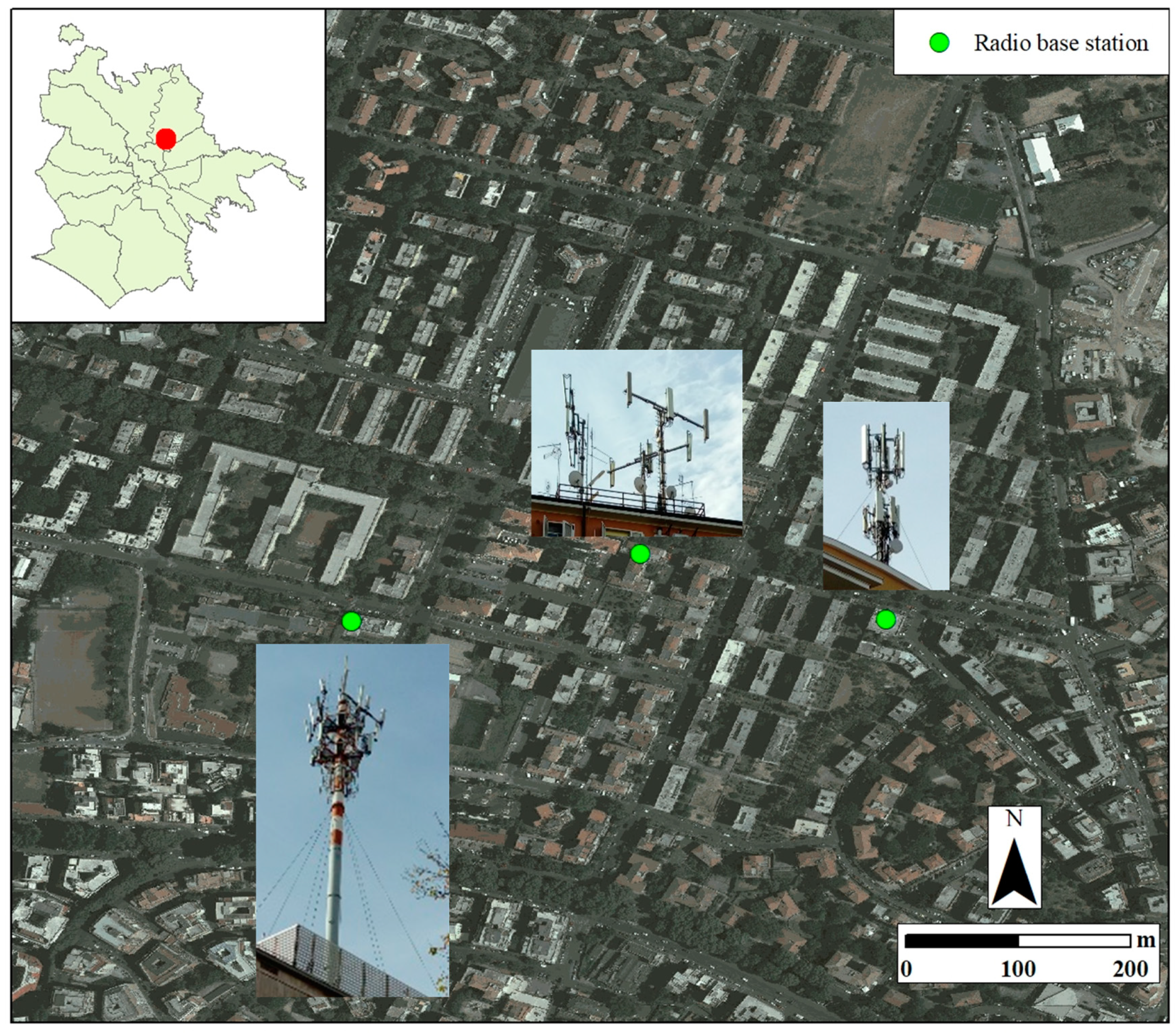
4.2. Exemplification No. 1

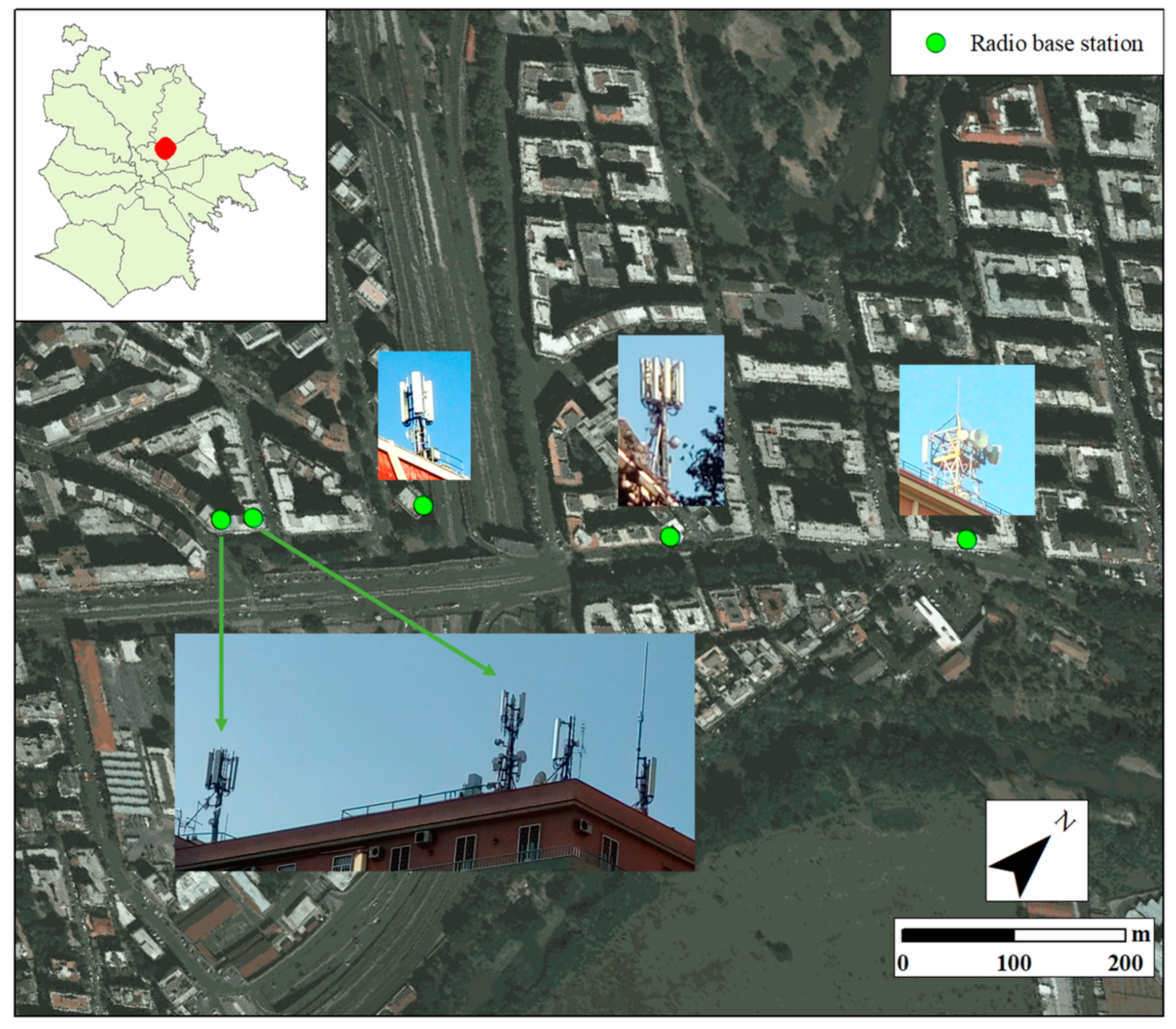
The first exemplification focused on an alignment of (probable) RBSs that are diffused on some buildings. During the field surveys, a certain thickening of RBSs of similar typologies was recorded in this lengthened surface portion with a particular density of antennas (subject to implementation) on the roof of the building on the left, near other high buildings. The different radio base stations were geolocalized and edited on an aero-satellite image (Figure 1), after having conducted some measurements of six minutes and a photograph relief.

In terms of applicative representation, for the first building on the left, with the aim of not weighing down and compromising the legibility of the elaboration and owing to the characteristics and vicinity of the antennas on the right, we considered two different points of origin for the buffer zones starting from this roof: one on the left and one on the right (where different elements were considered as elements of a unique integrated antenna). Then, there are two other buildings with an RBS each, and these antennas have a certain number of elements that are radially distributed. Finally, the building on the right is characterized by the presence of a structure made by radio links.

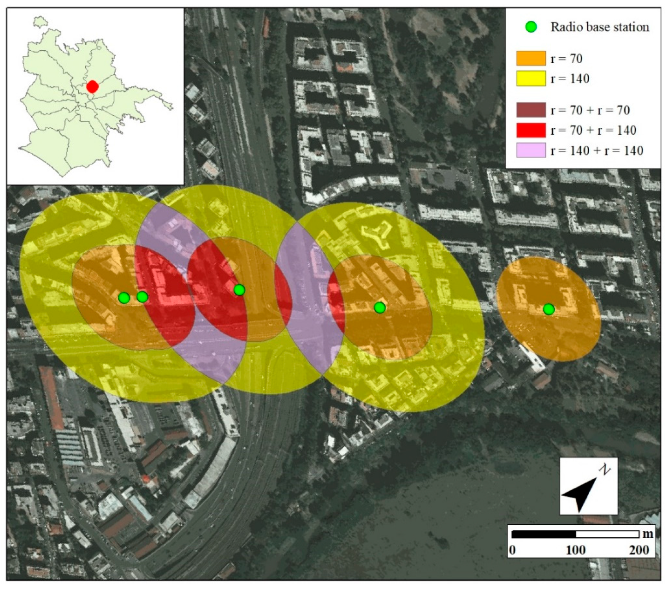
For all the RBSs located on the rooves of these buildings, with the unique exception of the building on the right, we defined two concentric circular buffer zones with radii of 70 and 140 m, while, for the antenna of the building on the right, we only edited a buffer zone of 70 m for the different types of structures (also considering the directions of radio links).

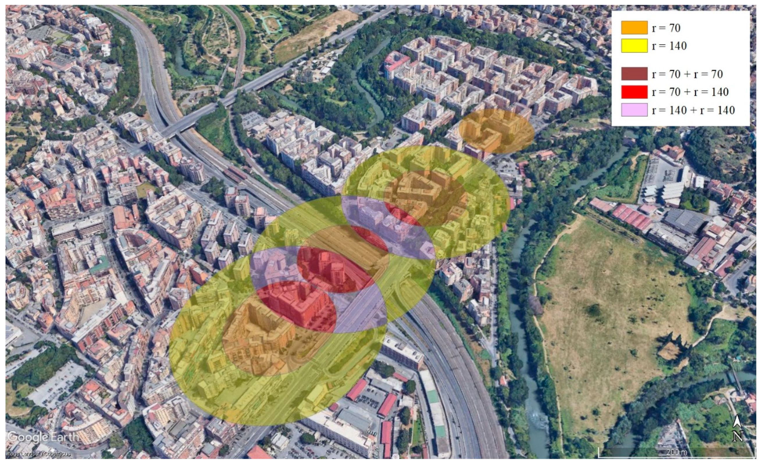
The GIS elaboration (Figure 2) and the prime three-dimensional model (Figure 3)—which provides an efficient visualization of the general situation, observable in detail with progressive zoom in, and giving emphasis to the territorial context characterized by a notable population density—evidenced the presence of different buildings (or parts of them), sometimes with notable dimensions, involved in the buffer zones with radii of 70 m, represented in orange; these buildings are therefore directly exposed to a distance that is smaller than should be expected. This elaboration also shows the presence of four red areas (dimensionally wider on the left) due to the intersection between buffer zones with radii of 70 m from an RBS and a buffer zone with a radius of 140 m from another RBS. These red secant areas are especially noteworthy because the buildings involved here are simultaneously exposed to electromagnetic fields coming from two different directions. Moreover, the elaboration also shows a very small strip of a secant area colored in brown (since it is a borderline case between two buffer zones with radii of 70 m from two different antennas) and with a maximum exposure level recordable on the basis of the verifiable possibilities. Furthermore, some buildings partially come into the pink areas due to the intersection between two buffer zones having a radius of 140 m from two different antennas.

In terms of discussion, we also have to consider that: the buildings situated in the vicinity of the two RBSs located on the building on the left record a condition of amplified exposure because the antennas are very near and there is a strengthened emission effect, which the automation process discloses as contiguous buffer zones in a unique solution and here there is as a kind of cumulated wave; in correspondence with the building on the right, we only considered a buffer zone of 70 m but a possible further level of precautionary attention could be considered, for example, with apposite measurements at a distance of some other value of tens of meters.

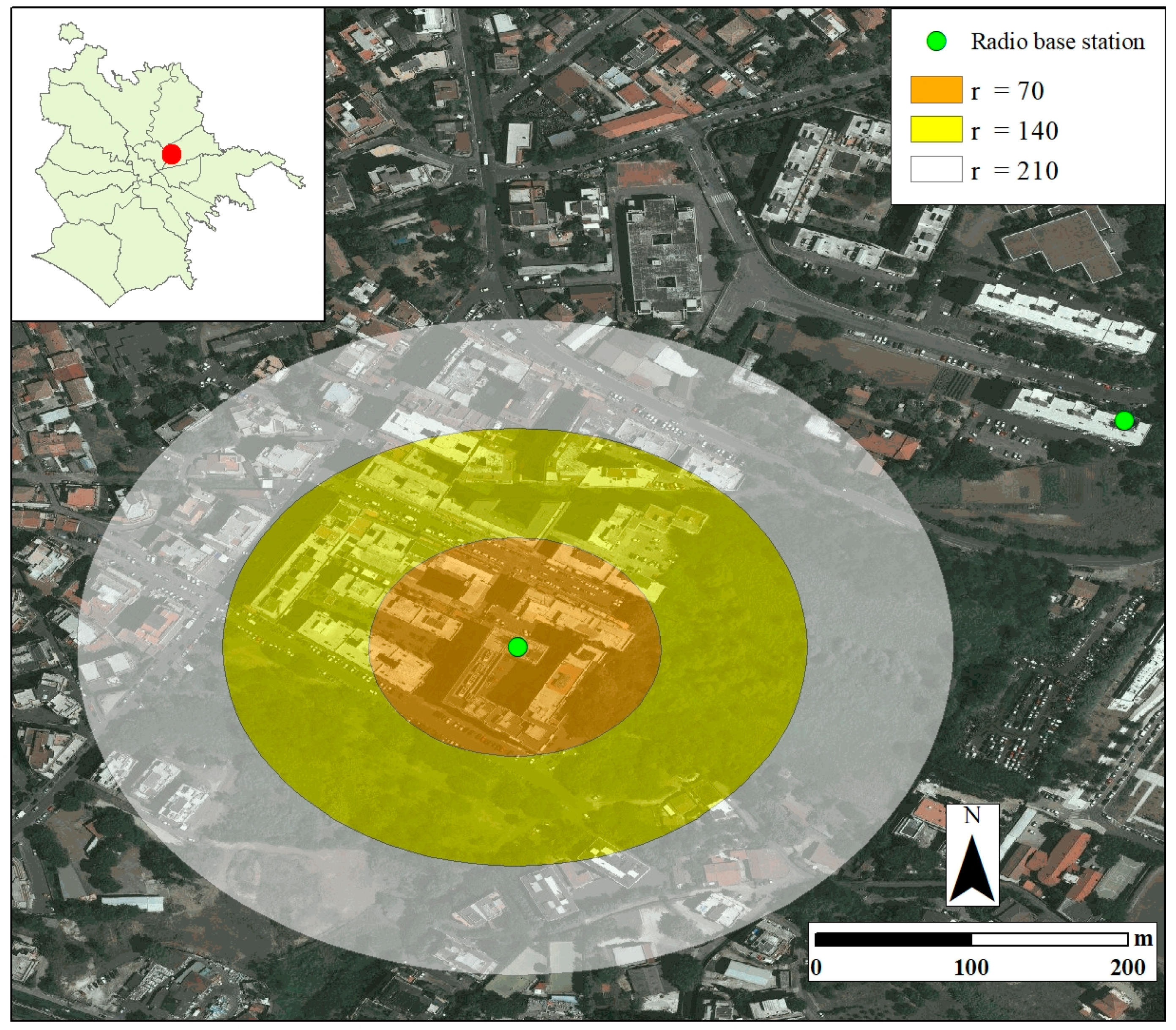
4.3. Exemplification No. 2

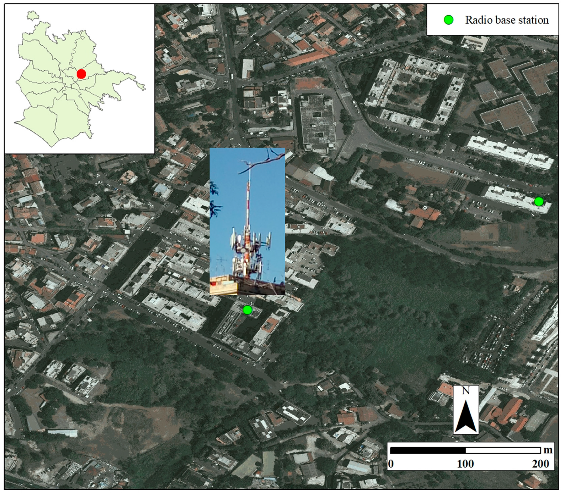
The second exemplification was focused on a context characterized by the presence of an imposing high antenna with the phenomenon of cositing and a high number of radial elements. This RBS was geolocalized and edited on an aero-satellite image (Figure 4) for the definition of three concentric circular buffer zones with radii of 70, 140 and 210 m. During the field surveys, we also recognized another RBS essentially made by three nearby antennas, of unique structures, with various elements each oriented in a specific direction and located on a wide horizontal axis. Nevertheless, for this application, we preferred to consider only imposing the RBS in order to represent the potential impact of such a considerable antenna according to a tripartition, without interferences coming from other RBSs. However, in the output product, we indicated this other antenna on the right, but without editing the respective buffer zones.

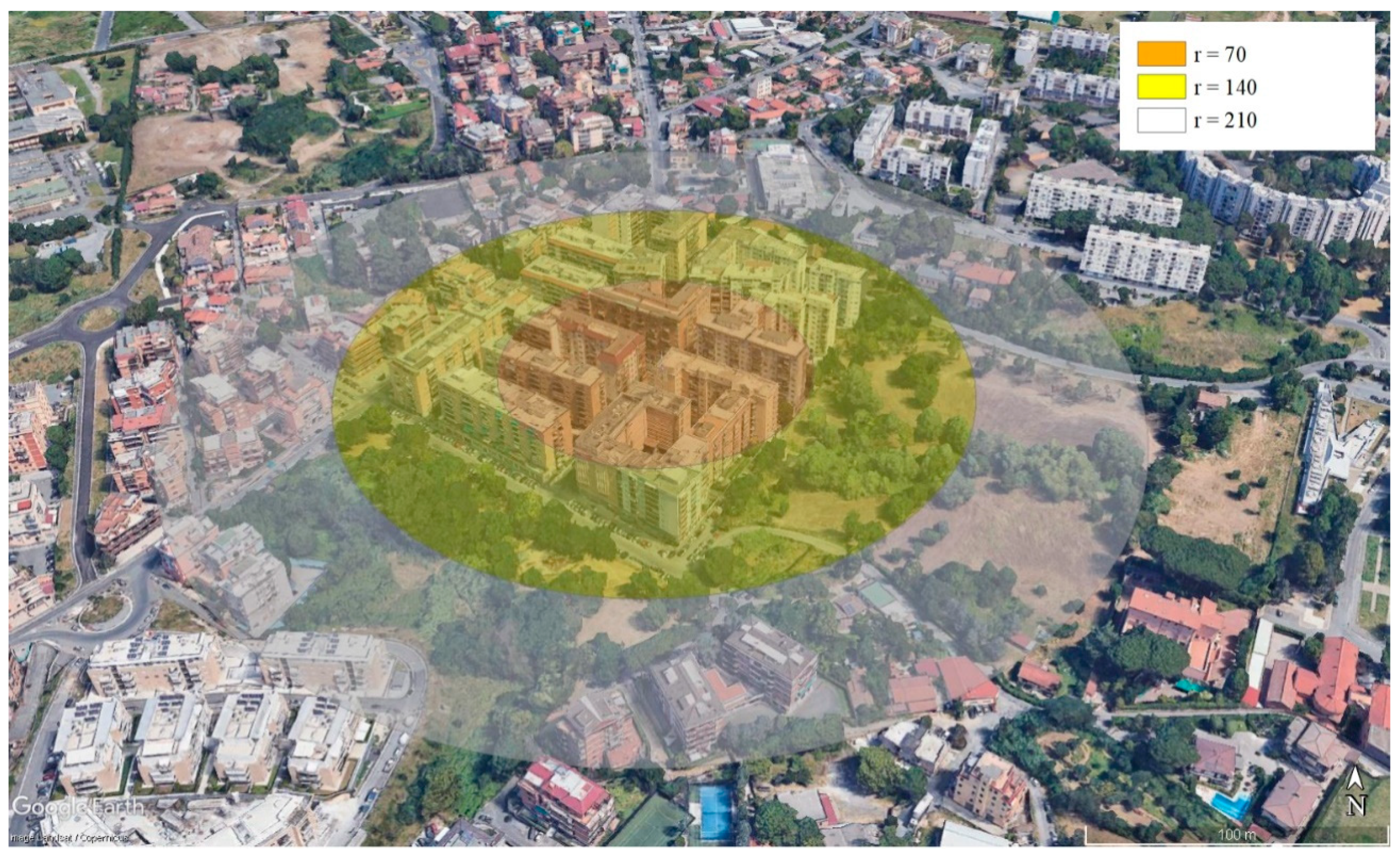
The GIS elaboration (Figure 5) and the prime three-dimensional model (Figure 6)—again produced through import and elaboration in Google Earth in perspectival view—show that some buildings’ facades are touched by the orange buffer zone with a radius of 70 m and they are set out in the sector coming from the west side to the north-east, while there are no other buildings in the remaining sectors that show spaces without constructions in the proximity. The same is roughly confirmed for the yellow buffer zone with a radius of 140 m (with the partial addition of a pair of buildings to the south-east). The definition of a further buffer zone, indicated in white and having a radius of 210 m, shows which zones and connected buildings should be kept under preventive control due to the typology of the RBS.

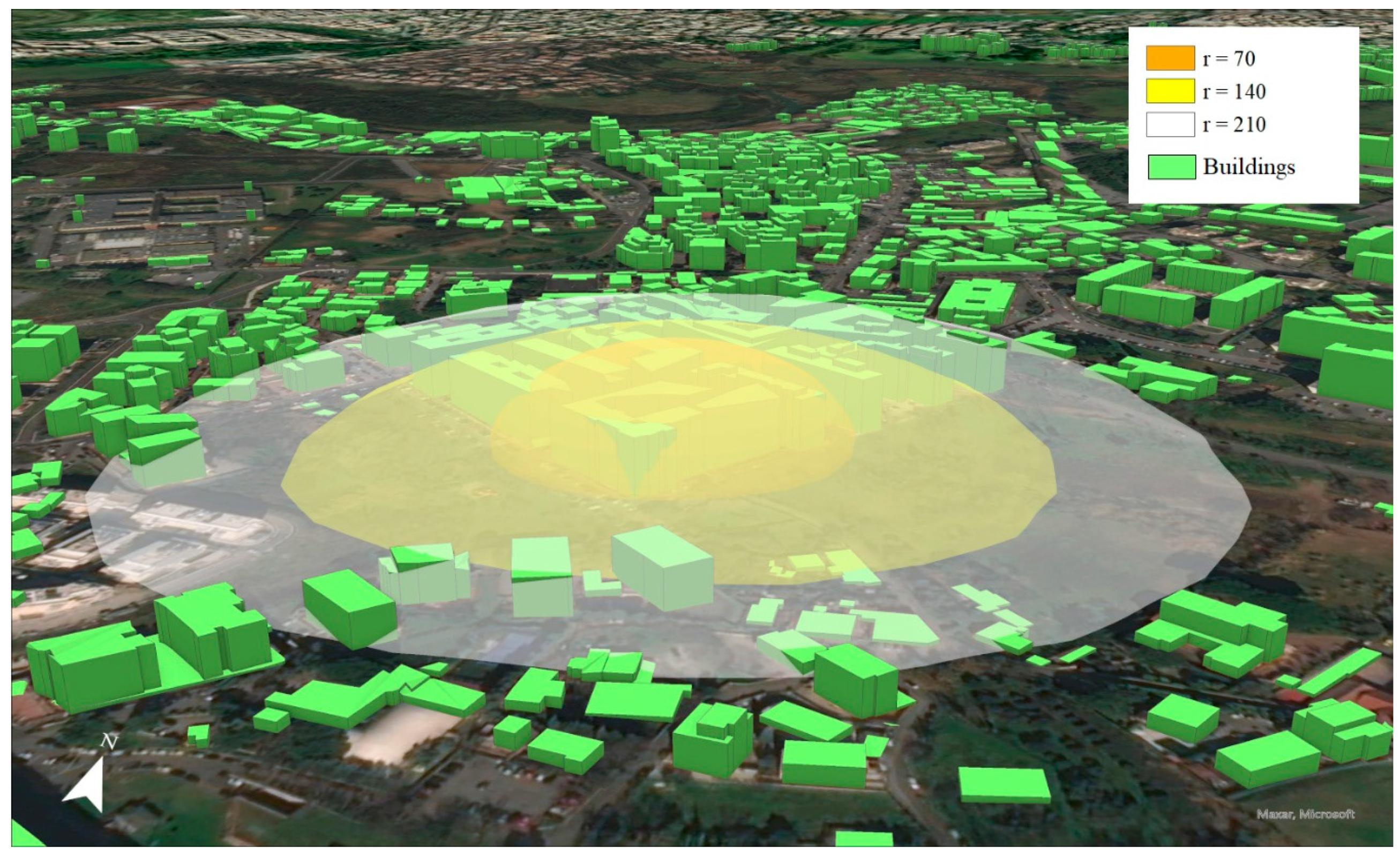
In this case—with minor technical complexity and visualization density for the choice of considering a unique RBS—we also tested the possibility of representing the buffer zones in terms of semispheres, proceeding toward a three-dimensional model where all the elements are reported as solid (Figure 7). For this purpose, we imported the model into ArcGIS Pro (2.6.2), where all the elements can be consulted in terms of volume and other information, i.e., collected in the Regional Numerical Technical Map (CTRN), as, for example, a building classification.

In order to represent the vertical decay of the buffer zones from a 3D perspective, one of the points from the observations feature class was used as an input for the Buffer 3D tool of the 3D Analyst toolbox, creating a 3D multipatch shapefile with the shape of a semisphere. As the Buffer 3D tool allows us to input a single buffer distance, this operation was run three times for the following radii: 70, 140 and 210 m, the same that were previously used for the Multiple ring buffer tool. Then, the feature classes were added to an ArcGIS Pro local scene, a newer desktop application from the ESRI ArcGIS for the Desktop suite of programs, whose features allow the handling of both 2D maps and 3D scenes from the same interface. Thus, their layers were edited with the use of the ArcGIS Pro modification tools, in order to move and scale the multipatch features to make them coincide with the top of the radio base station, as the spread direction of the waves tends to be downward.

A similar elaboration can be useful to provide further elements for the possible assessment of high exposure zones working in the phases of spatial analysis and query, also considering the possibility of evaluating the semisphere intersections among different radio base stations (in the case of secant areas). These operations, which create a certain visualization complexity and which are therefore useful during the steps of direct work in the GIS environment, can be suitable for the analysis of the hypothetical intersections since the RBSs have tilt angles (in fact their emission values in the building on which they are installed are minimal), and having in-depth data concerning the RBS characteristics concerning the reprojecting of the semisphere intersections in a further output product can show details that are otherwise not recognizable.

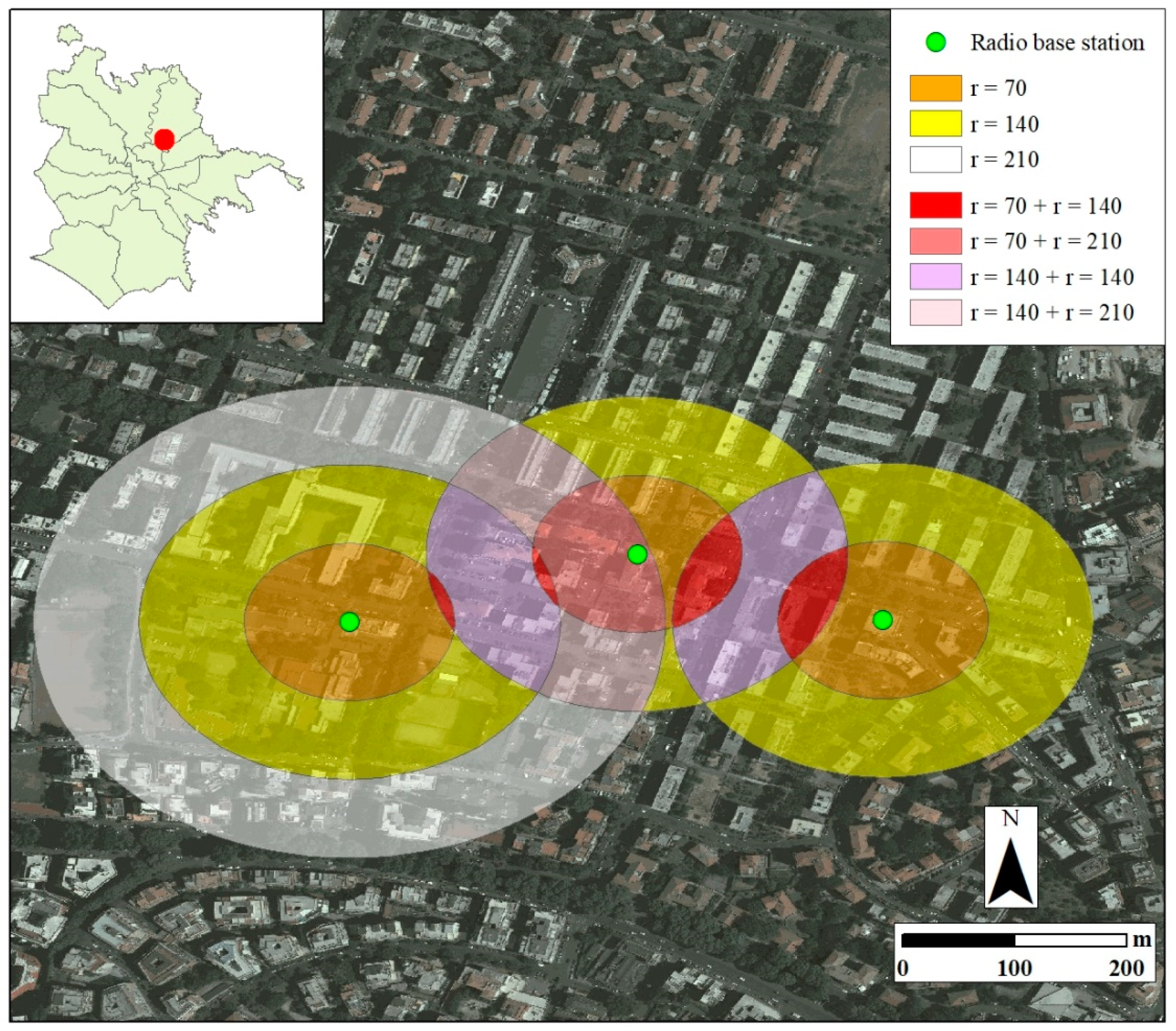
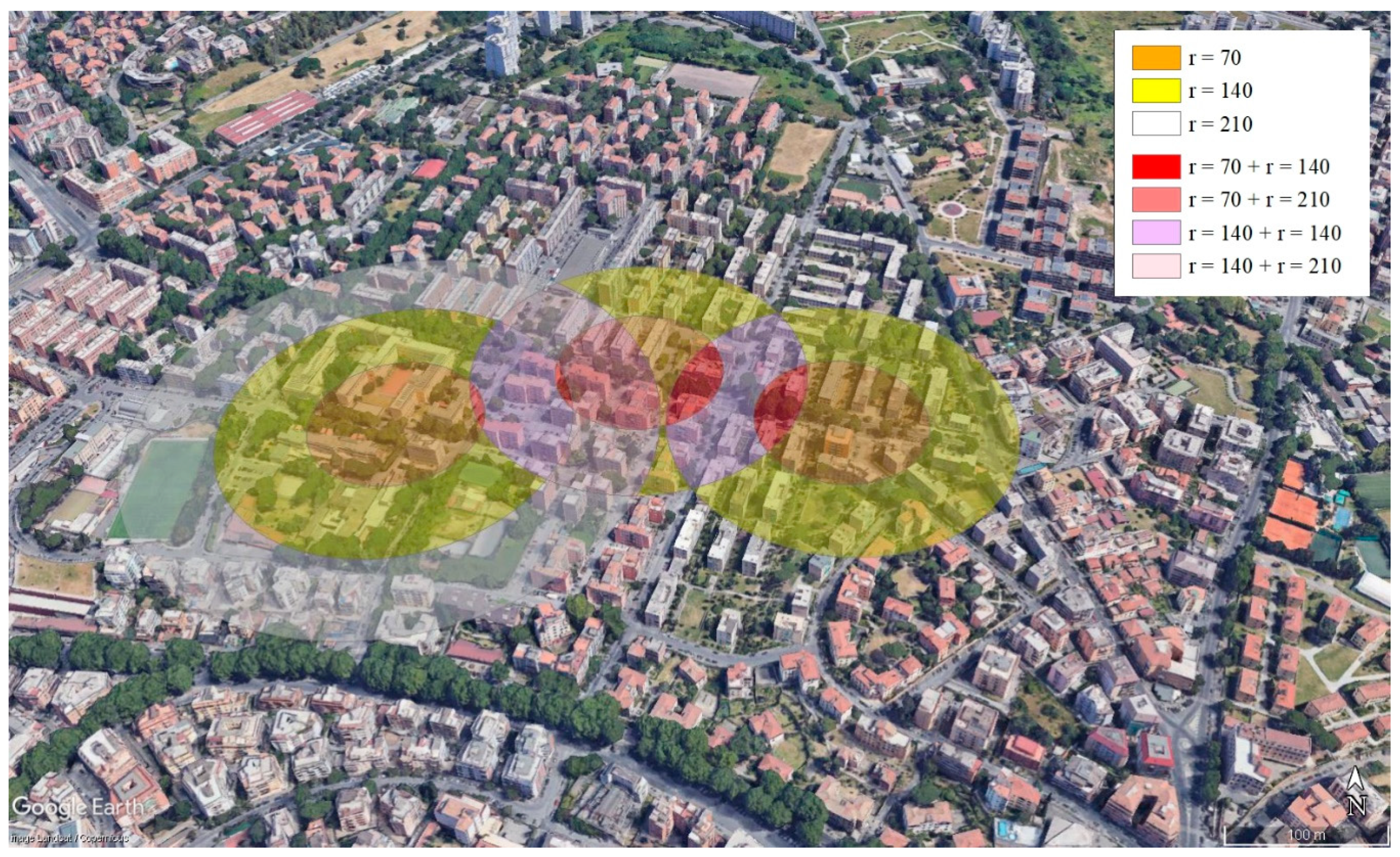
4.4. Exemplification No. 3

The third exemplification was focused on a territorial context where three different (probable) radio base stations—which constitute the vertex of an imaginary obtuse-angled triangle—were geolocalized and edited on an aero-satellite image (Figure 8) for the definition of the buffer zones. The RBS on the right is characterized by a cositing phenomenon on a unique antenna and we defined two concentric circular buffer zones with radii of 70 and 140 m. The RBS in the middle is essentially made up of three close antennas, of unique structures, with various elements each oriented in a specific direction and located on a wide horizontal axis; additionally, in this case, we edited two concentric circular buffer zones with radii of 70 and 140 m. The RBS on the left is an imposing high antenna with a repeated cositing phenomenon and we defined three concentric circular buffer zones with radii of 70, 140 and 210 m.

The GIS elaboration (Figure 9) and the prime three-dimensional model (Figure 10) show a very composite and articulate situation because there are many intersections among buffer zones having different radii and coming from different RBSs. First of all, there are several buildings involved in the radius of 70 m, and therefore in the orange buffer zones, since they are exposed over a distance that is less than should be expected. Then, there are four red areas (dimensionally wider on the right) due to the intersection between buffer zones with a radius of 70 m from one RBS and a buffer zone having a radius of 140 m from another RBS, and these areas show the presence of doubly exposed buildings due to a bidirectional interference. Moreover, there are two ample pink secant areas due to the intersection between two buffer zones having radii of 140 m from two different RBSs. Other buildings are involved in all the buffer zones with radii of 140 m and are represented in yellow. Due to the influence of the imposing antenna located on the building on the left, this elaboration also shows the presence of: a relevant number of buildings involved in the white buffer zone, having a radius of 210 m from the generatrix antenna; a certain number of buildings involved in a secant area between a buffer zone having a radius of 210 m from the imposing antenna and a buffer zone having a radius of 140 m from another antenna, represented in light pink; a certain number of buildings involved in a secant area between a buffer zone having a radius of 210 m from the imposing antenna and a buffer zone having a radius of 70 m from another antenna, represented in light red.

Therefore, the definition of a buffer zone with a radius of 210 m, in the case of imposing antennas, increases the possible verifiable situations, making the general interpretative investigation more complex but revealing further details and facets.

5. Open Conclusions

The applicative exemplifications produced for a study area of north-east Rome show the added value that can be recorded in terms of interdisciplinary analysis, urban modeling, interdisciplinary and multidimensional evaluations in an urban environment, with reference to: the identification of possible risk factors, localization alternatives, spatial decisions, health hazard reductions, ad hoc territorial planning and social utility. The attention of this paper has been place upon electromagnetic fields, due to the presence of some radio base stations, in order to provide inputs that highlight the importance of conducting extended GIS-based mapping, from a three-dimensional perspective, so as to feed innovative geographical analysis and support sanitary and epidemiological studies, finding a common denominator in the perspective of health as a public centrality and multidimensional approaches and multicriteria analysis based on original qualitative and quantitative data and geospatial models.

For the whole study area covered with the field surveys, we also produced a video that, from a bird’s eye view, makes it possible to enhance the localization perception of the radio base stations and the buildings involved in the different buffer zones, according to the perspective of a realistic 3D city model available for public geography, the involvement of institutions and awareness raising in the population.

The entire coverage of a municipality’s territory with a similar model, through bidimensional and three-dimensional applications in an upgraded GIS environment, is also able to produce a bird’s eye view video, based on the census of the all radio base stations (considered as source elements of electromagnetic fields by fixed structures), which makes it possible to have a dynamic and multiscale digital system functional for strategic planning and decision-making processes to address public health promotion and education, i.e., by identifying:

• areas with a probable high exposure due to the concurrence of different RBSs and/or the presence of imposing antennas, which are therefore particularly worthy of note;
• empty areas which have a relevant surface without antennas, probably due to the presence of another overloaded zone nearby, or a unique imposing antenna which covers a wide radius;
• areas which could be chosen for future installations are characterized by local conditions (topographical height, low level of urbanization in the close vicinity, etc.) which would make it possible to decongest and unload other zones;
• specific structures that do not have an adequate height that would require an increase in altitude because in the present state there are floors of nearby buildings that are directly too exposed.

In terms of other applicative possibilities, a similar GIS-based model can be reproposed, with methodological adjustments due do the different emission characteristics, frequencies and wavelengths, to other elements and polluting sources which produce electromagnetic fields—such as, for example, power lines, which have to respect specific different distances from houses and sensitive structures—that are sometimes very near residential buildings, schools and offices.

It is hoped that contributing to the development of a structured and organized system of risk factors and disease surveillance where georeferenced data can be examined and elaborated, in detail, using a GIS platform designed to alert institutions and public health workers to areas and groups of people who can be most greatly exposed to hazards and (in the future) record higher connected disease rates [47] (p. 52). The application of GIS-based analytical approaches to assess potential risk factors, monitor the outbreak of certain symptoms and diseases, predict and avoid possible critical situations and improve public health surveillance can promote the development of a digital health information system [10] (p. 20). A similar health information system would be able to provide the underpinnings for social utility decision-making through various key functions—from data generation to compilation, analysis and synthesis to communication and use [48] (p. 2)—in an environment able to elaborate cartographic solutions and test and process methods and models. After all, it has been recently evidenced that public health needs geography and its applied lens, first of all constituted by GIS, which opens up a wide range of opportunities in order to enrich scientific inquiry aimed at preventing problematic circumstances, disease outbreaks and their onset and at moving toward social utility [49].