Torrential Flood Water Management: Rainwater Harvesting through Relation Based Dam Suitability Analysis and Quantification of Erosion Potential

Abstract

In this study, a relation-based dam suitability analysis (RDSA) technique is developed to identify the most suitable sites for dams. The methodology focused on a group of the most important parameters/indicators (stream order, terrain roughness index, slope, multiresolution valley bottom flatness index, closed depression, valley depth, and downslope gradient difference) and their relation to the dam wall and reservoir suitability. Quantitative assessment results in an elevation-area-capacity (EAC) curve substantiating the capacity determination of selected sites. The methodology also incorporates the estimation of soil erosion (SE) using the Revised Universal Soil Loss Equation (RUSLE) model and sediment yield at the selected dam sites. The RDSA technique identifies two suitable dam sites (A and B) with a maximum collective capacity of approximately 1202 million m³. The RDSA technique was validated with the existing dam, Gomal-Zam, in the north of Sanghar catchment, where RDSA classified the Gomal-Zam Dam in a very high suitability class. The SE estimates show an average of 75 t-ha⁻¹y⁻¹ of soil loss occurs in the study area. The result shows approximately 298,073 and 318,000 tons of annual average sediment yield (SY) will feed the dam A and B respectively. The SE-based sediment yield substantiates the approximate life of Dam-A and Dam-B to be 87 and 90 years, respectively. The approach is dynamic and can be applied for any other location globally for dam site selection and SE estimation.

1. Introduction

Flooding is a global issue and is becoming a prime concern of research comprehensively. Flooding enriches grounds with minerals and sediments transported by water. These sediments increase the fertility of the soil and replace long-standing with new soil [1]. Floods are a great natural way to recharge groundwater [1,2]. Despite such benefits, when they cause human and economic loss, they are viewed as “catastrophes”. For better flood management researchers around the globe are dealing with procedures to utilize the flood water and control loss of assets. These studies presented structural and non-structural management of flood. The structural management considers physical measures including the construction of dams, leaves, floodwalls, and elevated buildings, cleaning of water bodies, and flood proving properties [3,4]. The second possible solution is non-structural, which includes planning for disaster, flood plain zoning, and early warning systems. These measures cannot completely utilize flood resources, this is the explanation integrated water resource management (IWRM) is standing out enough to be noticed [4].

Flash floods are a potential source of freshwater. However, flash floods are seldom considered as source of water due to the unavailability of management resources. Flash floods are different from traditional riverine floods in their extent and properties [5,6,7,8,9,10,11]. These floods last for a short time but are intense in the extent of destruction they cause. Resources from these floods cannot be as proficiently saddled as those from riverine floods.

Whereas, in the last few decades’, water consumption is rapidly increasing all over the world due to the increase in a population [12]. To supply reliable water resources, new water reservoirs have to be built to meet the fast-growing demands of water. Dams are the most important resources for the management of future water scarcity and a significant investment to provide essential services for the social communities [13,14,15]. Traditionally, dam suitability analysis is conducted using decision-making techniques. However, with the integration of remote sensing (RS) and geographical information systems (GIS), different techniques are evolving as the most appropriate approaches for dam site selection. The recent development in satellite RS has increased the power to investigate the terrain characteristics and hydrologic parameters. The integration of RS and GIS enhance the adaptability of joining the spatial data (geomorphology, topography, and geology) with numerical models and decision-making schemes including fuzzy logic, Boolean logic, weighted overlay, analytic hierarchy process (AHP), multi-criteria evaluation, and artificial intelligence [16,17,18]. Dam site selection was performed in the Greater Zab region of Iraq using AHP and fuzzy logic techniques. Another contemporary study in Sweden utilizes weighted overlay analysis on different layers (rainfall, evapotranspiration, geological, and geomorphological thematic maps) for dam site selection [18]. Further studies have also been conducted for dam suitability analysis using multi-criteria analysis [18]. Sayl et al. [19] integrates RS and GIS technique to estimate physical variable of dams (elevation-area-volume curve) in western desert of Iraq. Pandey et al. [20] process overlay analysis under Integrated Mission for Sustainable Development (IMSD) guidelines for dam site suitability in Karso, Hazirbagh, India. In a study Syst et al. [21] analyze soil conservation services curve number (SCS-CN) equation with compound weighted index (CWI) and multi criteria evaluation techniques in Sao-Francisco and Nile catchments to identify suitable locations for dam construction.

The primary ecological issue in the watershed zones is soil erosion (SE) which essentially influences the dam adequacy. SE accelerated by deforestation, overgrazing, and improper cultivation of land. Among the different factors, approximately 84% of SE is caused by water and wind [19]. However, the average soil loss estimated due to water is more than 2000 t-km⁻²y⁻¹ [22,23].

Worldwide, 0.5% to 1% of sedimentation every year influences the capacity limit of reservoirs. The expanded deforestation and destructing man-made exercises everywhere on the world anticipated that by 2050 most of the dams will lose their half of capacity [24]. In Asia, sedimentation has covered approximately 40% of the total storage of reservoirs [25]. The developing countries are also at high risk because sedimentation affects the long-term sustainability of storage structures. Iran is suffering from an annual average SE of 24 t-ha⁻¹y⁻¹ [25]. Approximately 30 to 32.8 Mha (million hectares) area is affected by SE through the water in India. In Pakistan, 16Mha land is affected by soil loss through different processes, and approximately 70% of soil loss 11.2Mha is categorized as erosion by water. Sedimentation in the three main reservoirs of Pakistan (Tarbela, Mangla, and Chashma) is going to reduce their storage capacities by over 40% in the coming years. Different studies show that SE has drastically affected the storage capacities of existing dams and reservoirs in Pakistan [26,27]. The production capacity of the Warsak dam in Pakistan has a 70% decreased due to SE [26].

Global trends show that more than 20 billion tons of sediment yield are accumulated in the ocean from the rivers [28]. Thus, the estimation of SE and sediment yield is important for new dam site selections and existing dams for life and storage capacity calculations. Conventional methods to assess SE risk is expensive and time-consuming [16,29]. The estimation of SE is improved with the development of the Revised Universal Soil Loss Equation (RUSLE) model [30,31,32]. The model has different input parameters related to the topography, climate, and cropping systems. Integration of GIS and RS tools are handy in the development of environmental models and their advanced features of data storage, management, analysis, and display. The factors of RUSLE are generated using modern techniques of GIS and RS [17]. The implementation of RUSLE for the estimation of SE based on the integration of GIS and RS was also used in different studies [33].

Torrential flooding and erratic behavior of rainfall in western catchments of Dera Ghazi Khan have created a myth for disaster risk reduction strategies. The unplanned urbanization and arid nature of the area further limited the availability of freshwater resources. Suitable site identification for dam construction is the utmost need for torrential flood management and to meet the water demands of the area. The study aims to provide effective management of hill torrents’ flow, converting the disastrous energy into a useful source by identification of suitable sites for storage structures. To select a group of indicators that exceedingly affect the dam suitability, different literature was investigated. The selected indicators follow hydrologic and engineering investigations in the spatial domain. The methodology adopted is based on the relation of selected indicators with reservoir and dam wall suitability. Focusing on the main problem of the area, the study also utilizes the GIS and RS technique to quantify the sediment yield and calculating the life of proposed structures.

2. Materials and Methods

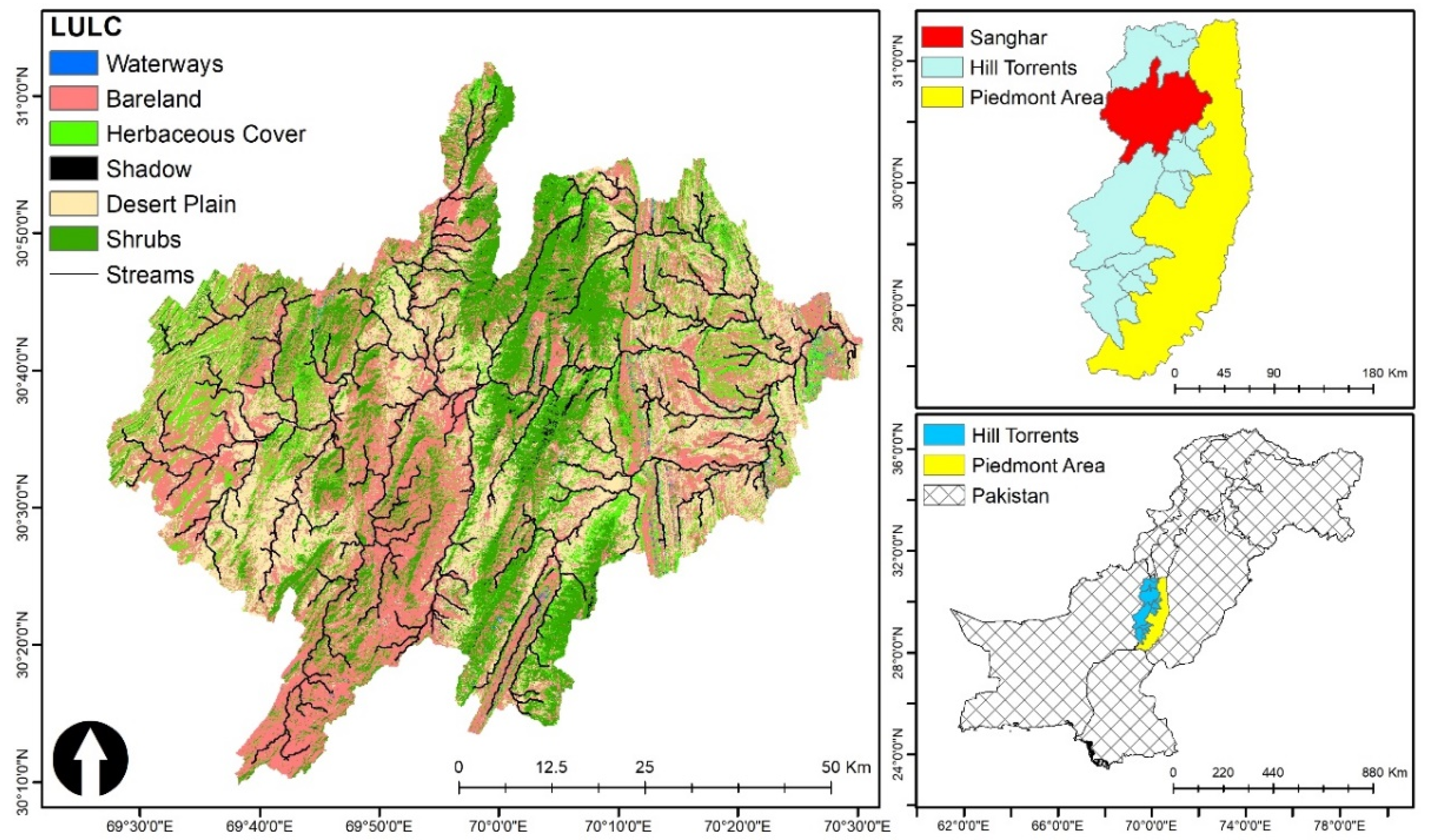
2.1. Study Area

Approximately, 200 hill torrents are counted that originate from the Suleman mountain range affecting Dera Ghazi Khan (D G Khan, Pakistan), Dera Ismael Khan, and Rajanpur districts. Among these torrents, 13 are classified as belonging to a major category as shown in Figure 1. These torrents are usually classified as small, medium, and major. The classification is based on average annual peak flows (small ≤ 5000; 5000 < Medium < 15,000; Major > 15,000) cfs [34]. The major torrents affecting D. G. Khan include Kaura, Vehowa, Sanghar, Sori Lund, and Vidor. The characteristics of torrents including; variation in peak flows, and high sediment yield hardened the management of these torrents [3].

The area is arid and water scarcity has not only limited agriculture but also socio-economic activities. During the monsoon season, flash flooding occurs and runoff generated by these torrential streams is far more than the local manageable capacity of farmers. The flows during monsoon season remain unutilized and frequently damage the low-lying urban settlements and patchy crops in piedmont plains [34].

The Sanghar is the most massive torrent in D G Khan District and the second-largest in the belt of D G Khan and Rajanpur districts with an approximate area of 4900 km². The area is divided into three physiographic regions including (i) Mountain range (catchment area), (ii) Pachad/Piedmont plain (plain between foothill and canal command area), and (iii) Canal command area (CCA).

The steep slope mountainous catchment is primarily majorly composed of loam, clay loam, and sandy clay loam. Desert plain and barren land cover a major part of Sanghar catchment. However, low-density shrub covers also exist in some parts of the catchment.

The torrential stream debouching onto the “pachad/piedmont area” from the Sanghar catchment. The stream locally named “Rod Kohi” is categorized as non-perennial and remains active in monsoonal season. The total length of the torrential stream is approximately 158 km [3,4,34]. The discharge data (

Table 1. Event frequency of Sanghar torrent.

Months	Avg. Discharge Cusecs	Min. Discharge Cusecs	Peak Discharge Cusecs	Total Events
March	15,482	3675	35,081	11
April	20,598	3675	38,045	13
May	23,046	10,394	60,901	18
June	22,817	3675	64,449	39
July	31,829	6751	146,300	94
August	29,984	3675	83,156	64
September	14,360	6751	24,064	9

) collected from Punjab Irrigation Department (2010–2019) shows that event concentration is clustered in the monsoon season (June, July, and August).

2.2. Geospatial Dataset

The data used for site selection were collected from different online and as well as from government organizations (

Table 2. Dataset used for dam suitability and Revised Universal Soil Loss Equation (RUSLE) model.

Source Data	By-Products	Suitability/Analysis	Examination	Resolution/Source
Discharge	Daily discharge	Event Frequency	Quantitative	Daily/Irrigation Department
DEM	Stream	Reservoir	Qualitative	5 m/Irrigation Department
		Dam Wall
	MRVBF	Reservoir
	TRI	Reservoir
		Dam wall
	Slope	Reservoir
		Dam wall
	CD	Reservoir
	VD	Reservoir
	GD	Dam wall
	Contour	Dam wall	Qualitative-Quantitative
		Reservoir
	LS	SE
GPM	R-factor		Quantitative	Daily-0.25°/Giovanni
Soil	Percentage Sand		Qualitative-Quantitative	250 m/soilgrid
	Percentage Silt
	Percentage Clay
	Percentage OM
Satellite Imagery (Landsat-8)	CP-factor			30 m/USGS-Glovis

). For dam site suitability analysis, digital elevation model (DEM) is the most important dataset. In this study, DEM product of 5 m spatial resolution was used to generate by-products indicators including multi-resolution valley bottom flatness (MRVBF), terrain roughness index (TRI), closed depression (CD), valley depth (VD), gradient to downslope (GD), and length slope factor (LS). The DEM product was collected from Punjab Irrigation Department.

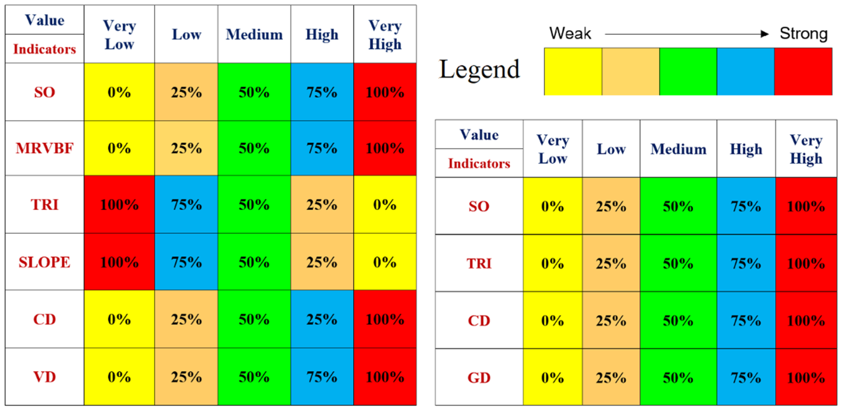
2.3. Indicator’s Relation and Suitability

The spatial suitability of storage structures is directly associated with morphometry and the terrain of the area. The indicators including stream ordering (SO), multiresolution valley bottom flatness index (MRVBF), terrain roughness/ruggedness index (TRI), slope, closed depression Index (CDI), and Valley depth (VD) thematic layers are used for reservoir suitability. However, TRI, slope, and downslope difference gradient (GD) were used for dam wall suitability analysis. The selection of indicators is solely based on the criterions defined by Munir et al. [4] and Stephens [31]. The criterions are a set of rules defined in the literature that should be followed for dam site suitability analysis. Each selected indicator represents certain criteria.

Stream ordering (1st criteria) was performed using the Strahler order scheme. It was of utmost importance to classify the streams in order to identify the length and position of the main channel in the study area. MRVBF index was developed by Gallant and Dowling [35]. The index classifies the flat bottom of valleys as low areas. Higher values of MRVBF represents the flat valleys along the stream. According to the defined relations, flat areas along the main stream were identified using MRVBF index (2nd criteria). TRI (3rd Criteria) quantifies heterogeneity-abruptness in the terrain over a specified length [36], is calculated as

$$\mathrm{TRI}=\frac{\mathrm{Elevation} \times \mathrm{Slope}}{\mathrm{Elevation}+\mathrm{Slope}}$$

(1)

Slope (4th criteria) of the area also impacts the site suitability analysis. The selected site should have gentle/low main slope values for reservoir and steep cross slope are suitable for dam wall [4].

Generally, the topography of the area commands the choice for the type of dam. A perfect gorge (narrow valley with steep cross-sectional slope) favors a concrete dam. However, rolling plains with wider valleys favors an embankment dam. The VD (5th criteria) and CD (6th criteria) indicators are utilized for the reservoir suitability, to examine the reservoir’s ability for water storage. CD indicator also represent the contour rule defined by [4,31]. However, the GD index quantifies downslope controls on local drainage [37]. The relationships of selected indicators with site suitability were defined based on a literature review [4,31,38,39,40,41] engineering as well as hydrologic investigations, and field expert’s counseling.

Buffer analysis is performed on the main ordered stream to develop a rectangular box unit. The box unit is 250 m in length along the mainstream and the width of the buffer is selected as 100 m; however, it may vary for different areas depending upon the topography of the mainstream. The average values of each indicator are extracted for n-box units along the mainstream and are classified into five classes based on their relationship as shown in Figure 2. The combination of yellow with 0% is the weakest relation with suitability and a red with a 100% effect gives a strong relation with site suitability. The classification of very low (VL) to very high (VH) is user-dependent and it can be replaced with numeric values ranging from 1 to 5.

The average extracted values of each indicator further analyzed using the simple additive weighting (SAW) technique for final decision making of storage structures. The technique solves the weighted performance of each indicator for individual box unit. SAW requires a normalization process either performed as a decision matrix or on the actual values. In this study, SAW technique was modified and performed on actual values of each indicator. The weight factor in SAW technique is divided into Inter weights (weights assigned to different indicators) and intra-weights (weights assigned to value/box units of individual indicators) categories. The technique follows the relation as under:

$$V={\displaystyle \sum }_{j=1}^n\left(W_{inter}\times W_{intra}^{rr}\right)r_{ij}$$

(2)

$$r_{ij}=\frac{X_{ij}}{ma{x}_{ij}}$$

(3)

• $r_{ij}=$ Normalized values of indicators
• $X_{ij}=$ Actual thematic layer values
• $W_{inter}=$ Inter weights between selected indicators
• $W_{intra}^{rr}=$ Intra weights for each box unit

The $W_{intra}^{rr}$ are calculated for all box units of selected indicators individually using the reciprocal rank technique. In this technique, weights are derived from the normalized reciprocals of ranks. The technique involves an ordinal number to each record/value rank, starting with the highest rank of 1 [42].

$$W_{intra}^{rr}=\frac{\raisebox{1ex}{$1$}\!\left/ \!\raisebox{-1ex}{$i$}\right.}{{{\displaystyle \sum }}_{j=1}^N\frac{1}{j}}$$

(4)

where $W_{intra}^{rr}$ is intra-weight using rank reciprocal, $i$ = individual value of the indicator, $j$ = ordinal number, and $N$ = total number of box units. Furthermore, $W_{inter}$ weights are assigned on equal weight strategy because the selected indicators influence equally on the selection of suitable site.

The final SAW output $\left(V\right)$ for each box unit is classified in ArcGIS 10.5 using standard deviation (SD) to minimize the manual dependency of users. The SD strategy makes the technique a widespread methodology where the dataset is free of specialists for arrangement and classification [43]. In the SD classification scheme, the number of classes is dependent upon the data spread and distribution. The symbology of classes is user-dependent. In this study, the number of classes generated through SD strategy further symbolized as very low (VL) to very high (VH). The combination of reservoir and dam wall suitable sites results in final output for storage structures.

2.4. Quantitative Analysis

The capacity and storage characteristics are required for the effectiveness of selected structures in flood scenarios. Elevation-Area-Capacity (EAC) curves are generated using (i) elevation surface area method designed for reservoirs and (ii) Trapezoidal rule implication for capacity calculation at each contour area [4,44,45]. The mathematical expression of the trapezoidal rule is given in the following equation:

$$V_t=\left(\frac{H}{2}\right)\times \left(A1+2.A2+2.A3+2.A_{n-1}+A_n\right)$$

(5)

$$H=\frac{(h_2-h_1)}{n}$$

(6)

where

$$h_2, h_1, n=\mathrm{value} \mathrm{of} \mathrm{the} \mathrm{largest}, \mathrm{smallest} \mathrm{and} \mathrm{total} \mathrm{number} \mathrm{of} \mathrm{contour}.$$

2.5. Sediment Analysis and Dam Life

Sediment erosion (SE) analysis is performed using the RUSLE equation to calculate the life of proposed structures in the area. The technique is an empirical approach for predicting the long-term rate of erosion potential expressed as a function of five indicators including (i) rainfall erosivity (R), (ii) soil erodibility (K), (iii) slope length and steepness (L and S), (iv) support practices (P), and (v) cover management practices (C) inputs [46,47,48]. The Sanghar catchment area mostly consists of a barren mountain with little or no cropping system. Therefore, the average SE values are mainly or solely depending upon the LS, R, and K factors.

$$\mathrm{SE} \left(\mathrm{t}-{\mathrm{ha}}^{-1}{\mathrm{y}}^{-1}\right)=\mathrm{R}\times \mathrm{K}\times \mathrm{LS}\times \mathrm{C}\times \mathrm{P}$$

(7)

The multi-source gathered and created parameters of RUSLE equation with various spatial resolution goes through bilinear resampling measure. The cycle ascertains the estimations of every pixel by averaging the values of encompassing four pixels. The resampling cycle permits to downscale the precipitation raster to coordinate the spatial resolution with other datasets.

2.5.1. Rainfall Erosivity (R) Factor

The intensity and extent of every single rainfall event are expressed as R factor. Satellite rainfall data on daily time scales of GPM (global precipitation measurements) product is used for the calculation of R factor. The product is widely used due to its enhanced accuracy. The gauge data of nearby stations (D.G. Khan) is used to validate the satellite data. In this study, R-factor was calculated using the proposed scheme of [49].

$$\mathrm{R}=k·{{\displaystyle \sum }}^{ }{\left(P_d\right)}^a$$

(8)

where coefficient $k$ and exponent $a$ are model parameters, and $P_d$ is daily precipitation. The R is calculated with daily precipitation for all days $P_d>0$ in a month is summed. However, coefficient $k$ varies both spatially and temporally [50]. Ref. [51] showed that exponent $a$ is close to 2, while a number of empirical approaches substantiate the value of $a$ between 1.5 and 2 [52].

2.5.2. Soil Erodibility (K) Factor

The soil susceptibility to erosion due to rainfall and generated runoff is justified by the K factor. The factor is calculated from different empirical equations [53,54] incorporating the soil properties like percentage organic matter, soil texture, and permeability.

$$\mathrm{K}=27.66 \times m^{1.14}\times {10}^{-8}\times \left(12-a\right)+\left(0.00043\times \left(b-2\right)\right)+\left(0.0033\times \left(c-3\right)\right)$$

(9)

where $a, b, \mathrm{and} c$ are percentage organic matter, soil structure code, and soil permeability code, respectively.

However, the percentage content of organic matter (OM) is related to organic carbon (OC) content. OM content is calculated using the relation defined by [55,56]. The percentage of sand, silt, clay, and organic carbon is collected from soilgrid and Harmonized World Soil Database (HWSD). The factors $b$ and $c$ are calculated using soil texture classification [57]. The classification is based on the texture of sand, silt, and clay content as shown in

Table 3. Coarse to very fine soil classification.

	Rules-Content is in %	Status	$\mathit{b}$
OM > 20%	-	Organic	-
OM ≤ 20%	Clay > 60	Very Fine	1
	Clay ≤ 60 & > 35	Fine	2
	Clay ≤ 35 and Sand < 15	Medium Fine	3
	Clay ≥ 18 & ≤ 35 and Sand ≥ 15 & ≤ 65	Medium	3
	Clay < 18 and Sand > 65	Coarse	4

.

Factor $m$ in the above equation represents the texture percentage of soil as:

$$m=\% \mathrm{of} \mathrm{Sand}+\% \mathrm{of} \mathrm{Silt} \times \left(100-\% \mathrm{of} \mathrm{clay}\right)$$

(10)

2.5.3. Topographic LS Factor

The LS-factor explains how topography affects the SE process. The L and S factors describe the impact of slope length and slope steepness respectively. The required SE model is calculated through the combined L and S factors (LS-factor). The slopes greater than 9% are more prone to soil loss [58]. The methodology adopted the Renard et al., 1997 [59] algorithm for the estimation of the S-factor based on slope gradient.

$$\mathrm{S}=10.8 \times sin\theta +0.03, \mathrm{where} \mathrm{slope} \mathrm{gradient}<0.09$$

(11)

$$\mathrm{S}=16.8 \times sin\theta -0.5,\hspace{1em}\hspace{1em}\mathrm{where} \mathrm{slope} \mathrm{gradient} \ge 0.09$$

(12)

where $\theta$ is a slope in degrees

The L-factor is calculated using the model proposed by Desmet and Govers 1996 [60]. The model extended Foster and Wischmeier’s 1974 [61] approach to a 2-dimensional terrain [62].

$$A=\frac{{\left(A_{i,j-in}+G^2\right)}^{m+1}-A_{i,j-in}^{m+1}}{G^{m+2}\times {\left(sin{\alpha }_{i,j}+cos{\alpha }_{i,j}\right)}^m\times {22.13}^m}$$

(13)

where $A_{i,j-in}$ the area is contributing to the inlet grid cell $\left(i,j\right)$ measured in m². $G$ is cell size in meters. ${\alpha }_{i,j}$ is the aspect of the grid cell $\left(i,j\right)$. However, $m$ is related to the ratio of the rill to interill erosion (β).

$$m=\frac{\beta }{\beta +1}$$

(14)

and

$$\beta =\frac{\frac{sin\theta }{0.0896}}{\left[0.56+3\times sin{\theta }^{0.8}\right]}$$

(15)

$\theta$ is a slope in degrees. The value of $m$ ranges from 0 to 1 [62].

2.5.4. Cover (C) and Control Practice (P) Factor

The impact of landcover on soil erosion is estimated using C-factor. The satellite data of Landsat-8-Operational Land Imager and Thermal Infrared Sensor (OLI/TIRS) was used for pixel-based LULC (Land use land cover) classification. The available cloud free Landsat images were acquired for 3 March 2020. The Sanghar catchment was covered in two Landsat images of Paths 152, and 151 and Row 39. The images consist of nine spectral bands with a spatial resolution of 30 m. The band 2 to 7 (visible to short wave infrared) were stacked and mosaiced to generated a multiband composite satellite image of the study area. The training sample from mosaiced image were collected and clustered by analyzing the identical spectral behaviour of pixels. The sample pixels with identical spectral behavior were labelled to the particular LULC class. The multiband composite image with different clustered training samples was further processed in Erdas Imagine 2014 using ML (maximum likelihood) algorithm for LULC classification. The ML algorithm assumes that the statistics for every class in each band are normally distributed and calculates the probability that a given pixel belongs to a selected class. Each pixel is assigned to the LULC class that has the highest probability. The values of the C-factor against each LULC class were collected from [63,64] and were then joined with classified raster. The

Table 4. C-factor values.

Sr. No	Land Cover	C-Factor
1	Bare land	1
2	Desert Plain	0.97
3	Herbaceous Cover	0.7
4	Shrubs	0.6
5	Waterways	0.98

shows the assigned C-factor values for each LULC class.

The exercises/practices to minimize erosion are described by P-factor. The Sanghar catchment is a hilly catchment and has never been practices for erosion management; subsequently P-factor is taken as 1 for the whole catchment.

2.6. Sediment Yield (SY) and Sediment Delivery Ratio (SDR)

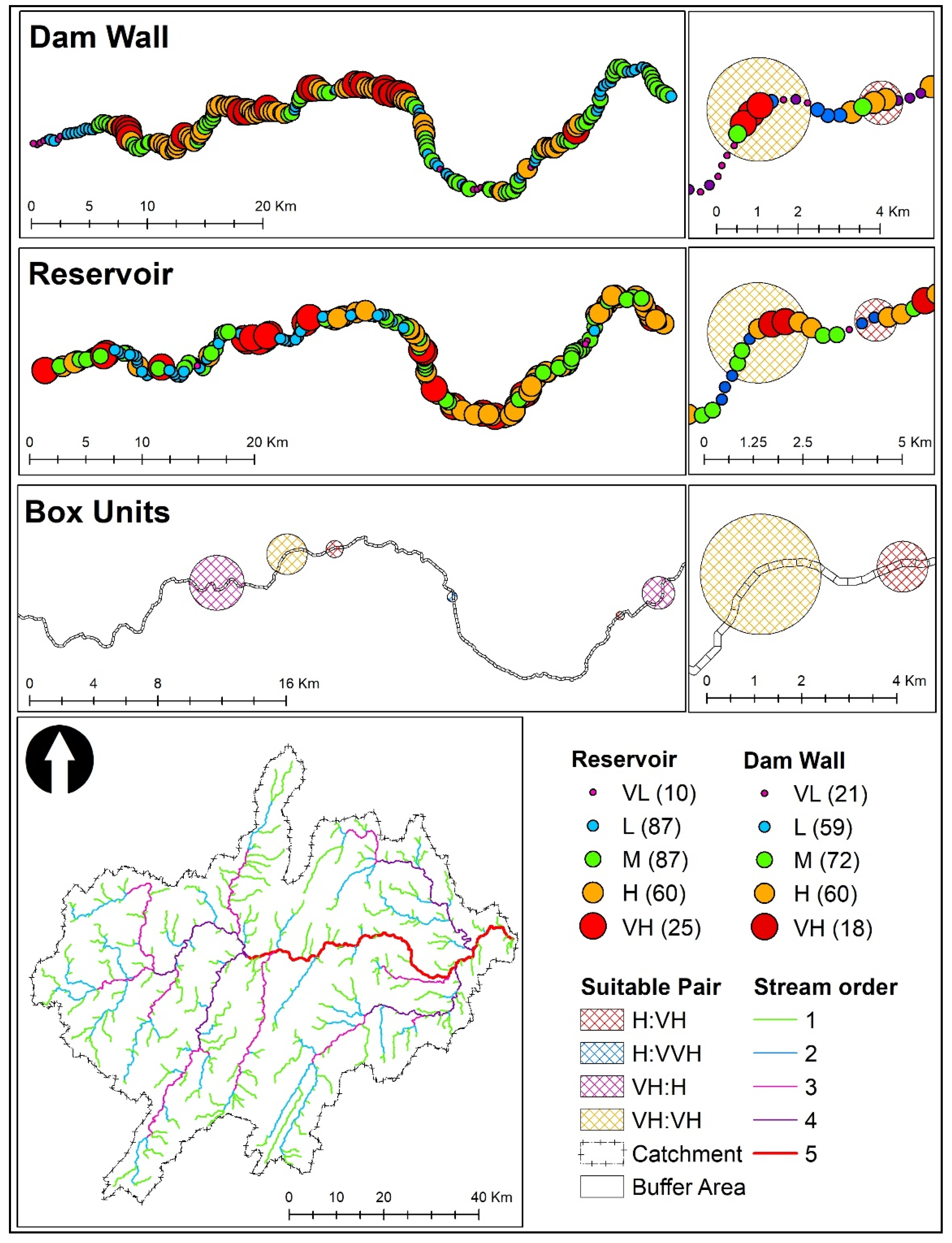
The SY is the gross SE delivered to a specific location. The SDR estimates the extent to which SE is stored in an area. SDR is the ratio of SY to SE of a basin. The SDR was calculated using empirical relation developed by Sharda and Ojasvi 2016 (Equation (16)) [64]. The relation was modified by Swaarnkar et al., 2018 (Equation (17)) [48].

$$\mathrm{SDR}=1.817 \times A^{-0.132}$$

(16)

$$\mathrm{SDR}=1.42\times A^{-0.132}$$

(17)

and

$$\mathrm{SY}=\mathrm{SDR}\times A$$

(18)

where $A$ is the area of basin/watershed/catchment.

The Sanghar catchment was further sub-divided into smaller 133 sub-catchments according to the drainage density of the area. The SY was calculated at the sub-catchment level. The division into smaller sub-catchment allows the SY estimates at a different location using SDR and SE of individual sub-catchment. The process was followed to calculate the SY at the proposed dam sites.

The area under study is an ungauged catchment with no sediment measurements. The methodology was verified with the adjacent catchment of Vidor. A project on Vidor torrent was initiated in 2016 for sediment measurements by the Punjab Irrigation Department, Pakistan. With the limited number of records, the SY results were compared with the observed SY records.

3. Results

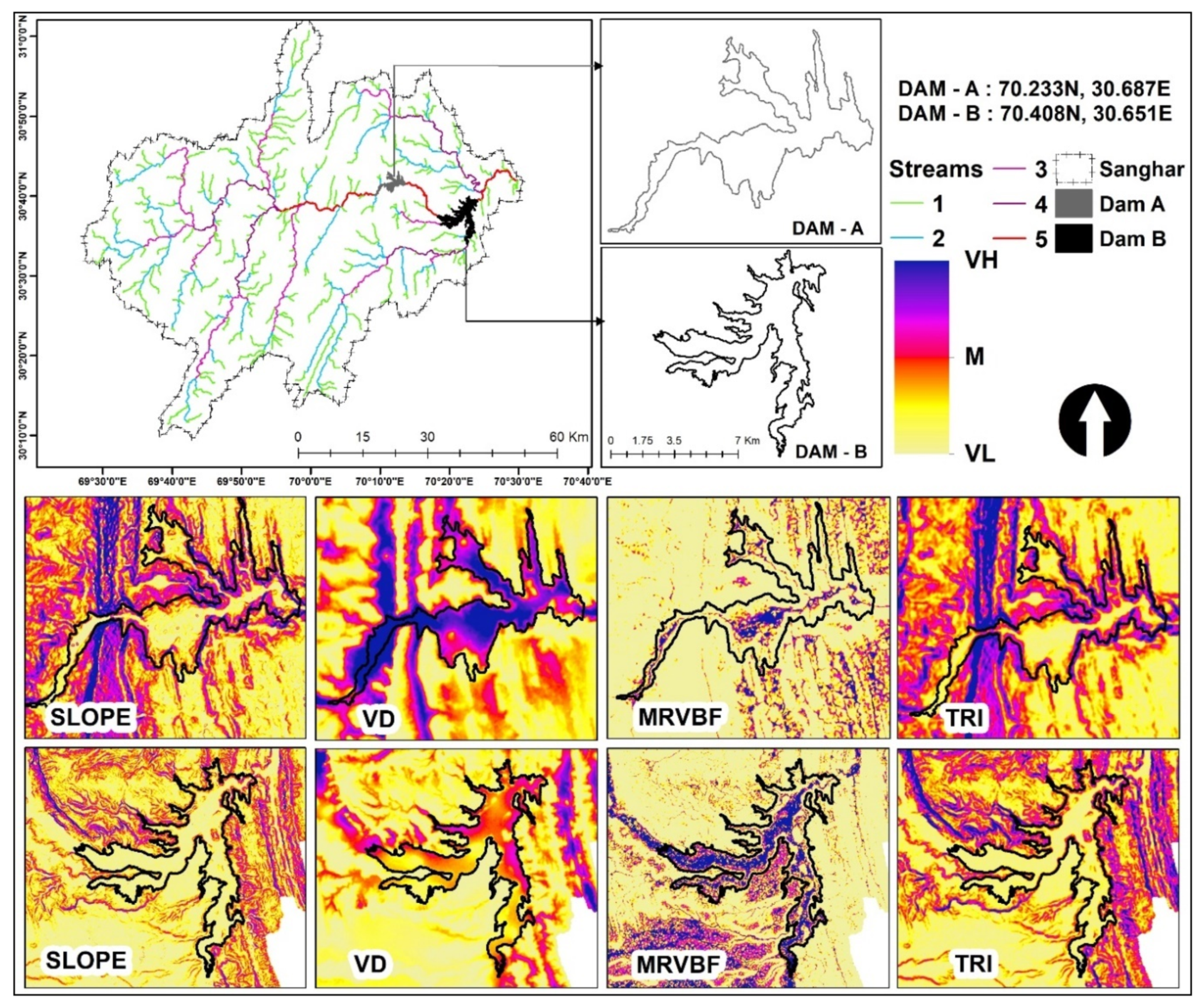
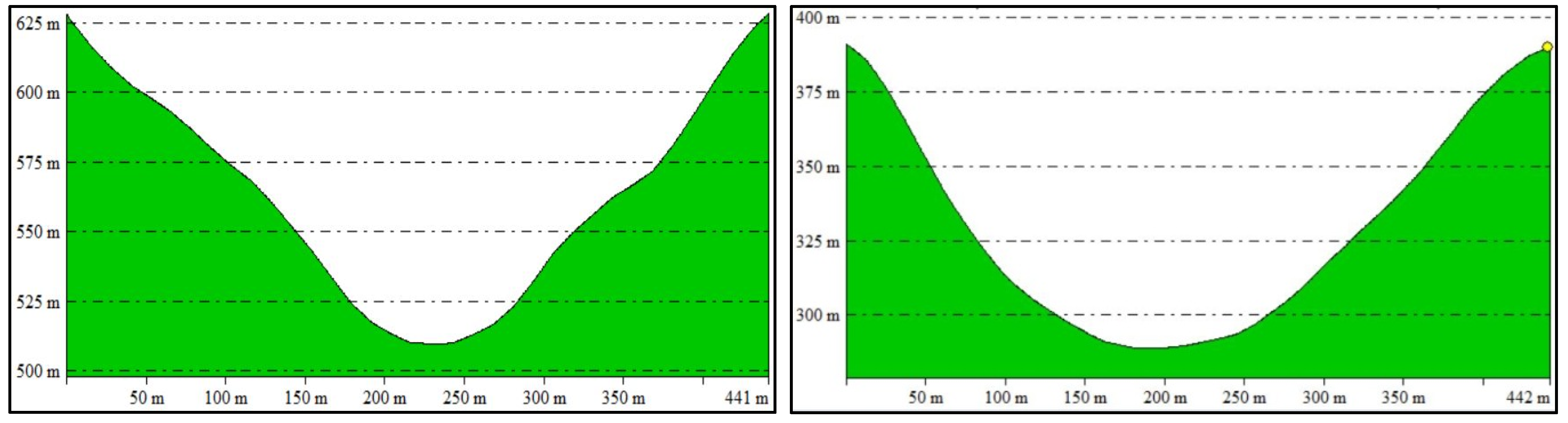
3.1. Dam Suitability

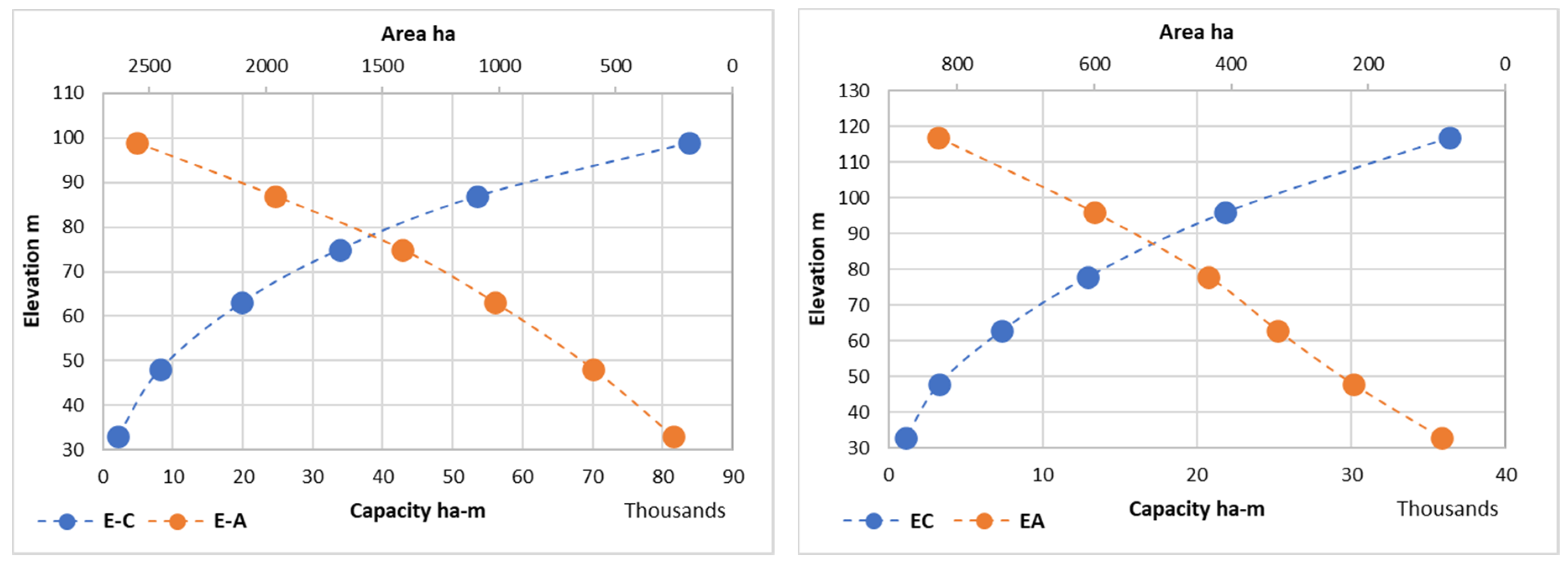
The selected indicators show the skewed distribution for 269 box units along the mainstream. The positively skewed nature of indicators restricts the recurrence of high values in the catchment. The mean and standard deviation of all indicators substantiates high frequency of low to medium range of values. The skewed nature of indicators was observed due to the high ridges and heterogeneity in the area. The statistics of all indicators are shown in the

Table 5. Statistical summary of Indicators.

Indicators	Mean	Standard Deviation	Minimum	Maximum	Distribution
Slope (degree)	12.25	9.82	0	81.19	Skewed
TRI	7.22	5.84	0	125.09	Skewed
MrVBFI	0.267	0.552	0	4.98	Skewed
CDI	1.24	1.53	9 × 10−4	79.03	Skewed
VD (m)	39.55	35.034	0	364.19	Skewed
GDI	0.266	0.142	0.056	1.44	Skewed

.

Based on the defined relations of indicators followed by inter and intra weights incorporated in the SAW technique, two sites were identified as most suitable for flash flood water management. The sites were selected from five suitable combinations of reservoir and dam wall as shown in Figure 3.

As per the Strahler classification scheme, the Sanghar hill torrent is composed of five stream orders with 5th as the main channel. Dam-A is located upstream of Dam-B on the fifth ordered stream (first criteria). The two suggested sites are approximately 22 km apart. The proposed site for Dam-B is considered as the main dam with a much higher capacity as compare to Dam-A. The reservoir areas of selected sites contain high to very high values of the MRVBF index (second criteria). However, TRI results substantiate low values in the reservoir area and high values for the dam wall (third criteria). The behavior of TRI shows that reservoir comprises of homogeneous topography as shown in Figure 4.

The reservoir areas of both sites show very low value (<5%) along the reservoir and high to very high values (100% < slope < 120%) for the dam wall respectively (fourth criteria). The sites were selected with large catchment areas to accumulate maximum flash flood water. Among the 269 box units on main order stream 25, and 60 area classified in very high, and high classes respectively for the reservoir suitability. However, 18, and 60 box units are classified in very high, and high class respectively for dam wall suitability. The topographical summary of the proposed sites is shown in

Table 6. Summary of selected suitable sites.

Dam	Max. Height m	Top Width m	Reservoir Area at Max. Height-ha	Catchment Area Mha	Capacity Mm3	Elevation of Base Contour m	Cross Slope Degree	Stream Order
A	117	445	828	0.299	363.92	513	45–55	5th
B	99	436	2554	0.405	838.42	291	42–50	5th

.

CD, VD, and contour along the main channel were analyzed to identify the best gorge in the area (fifth, and sixth criteria). A gorge is classified as a narrow valley with steep cross slopes located between hills or mountains. The selected sites represent a narrow opening with a large reservoir area having the capability to accumulate maximum water with minimum dam wall construction. This will allow the selected sites to accumulate maximum water with narrow opening. The mountainous topography of the area substantiates natural existence of perfect gorges along the main ordered stream. The cross-sectional profile of the dam’s wall is shown in Figure 5.

3.2. EAC Curve

The contour analysis of suitable sites was performed for EAC curve formation. The surface area and capacity at individual contour elevation was calculated. The selected site for dam-A consists of a maximum of 39 contours with a 3 m interval (39 × 3 = 117 m) having a base contour elevation of 513 m.

At the maximum designed height of 117 m, the Dam-A has the capability to store 363.92 Mm³ of floodwater with a surface area of 828 ha. Similarly, Dam-B has a base contour elevation of 291 m. At the maximum designed height of 99 m, Dam-B consists of 33 contours with a storage capacity of 838.42 Mm³ as shown in Figure 6. The reservoir area of Dam-B at maximum height is much larger than Dam-A. However, Dam-A has a higher potential of maximum height than Dam-B.

3.3. Soil Erosion (SE)

First, the different factors of RUSLE are presented followed by SE estimations. The results are average values based on the past six-year record (2014–2019) as shown in Figure 7.

3.3.1. R-Factor

The effect of the R-factor for the estimation of SE is averaged out over the selected period. The areas with a higher altitude, particularly mountainous catchments, receive high rainfall. The study area is a part of the mountainous range with varied topography from upstream to downstream. The R-factor shows that the rainfall rate is higher around the ridge in the center of the catchment with a height > 2000 m. The value of the R-factor ranges from 1073.75 to 2418.49 from low to high, respectively. Low rainfall values show low erosivity in the eastern part of the catchment. The R-factor gradually reduces in the downstream relatively low elevated areas. The R-factor varies considerably for different storm intensities.

3.3.2. LS-Factor

Due to the mountainous nature of the catchment, LS-factor shows a high influence on SE results. The results show higher values of cells on the ridge and adjacent areas (13 ≤ LS ≤ 20.5). The higher values for ridge areas can be due to the steep slope (S-factor). However, relatively higher values of LS-factor were also observed for the cells close to the main channel (fifth order). This is mainly due to the large values of stream accumulation/contributing area (L-factor). Low values of LS-factor (<2) in the patchy pattern were observed for the rest of the catchment. The variation for the other parts of catchments was observed between 2 and 12.

3.3.3. K Factor

The soil map shows the presence of clay loam in the eastern part and patches of sandy clay loam in the catchment; the rest of the catchment is mainly covered with loam. Typically, the loamy soil is considered more susceptible to erosion as compared to the other classes. K-factor calculation also involves the percentage of OM content in the soil. OM increases soil fertility and stability. The OM results show a patch of higher values (2 ≤ OM% ≤ 3.57) in the north of the catchment, however, small values of OM (<1) exist in patches; the rest of the catchment contains a spatially variable range of OM between 1 and 2. The percentage silt, sand, clay and OM content results in K-factor ranges from 0.016 to 0.034. The area is mostly of loam soil, spatial variation of high silt content along the loam soil reflects the high values of K-factor.

3.3.4. C Factor

The LULC suggested C-factor values mentioned in Table 4 show that 1 for bare-land and 0.97 for desert plain covers 1826.7 km² and 1209.2 km² areas, respectively. Higher values of the C-factor increase the vulnerability to soil erosion. However, the rate of soil erosion decreases with vegetation cover. The vegetation cover improves the physical and chemical properties with the increase in the percentage of OM and provides the barrier to eroded soil. Herbaceous cover (C-factor = 0.7) and shrubland (C-factor = 0.6) covers 673.4 km² and 985.8 km² area of the Sanghar catchment, respectively.

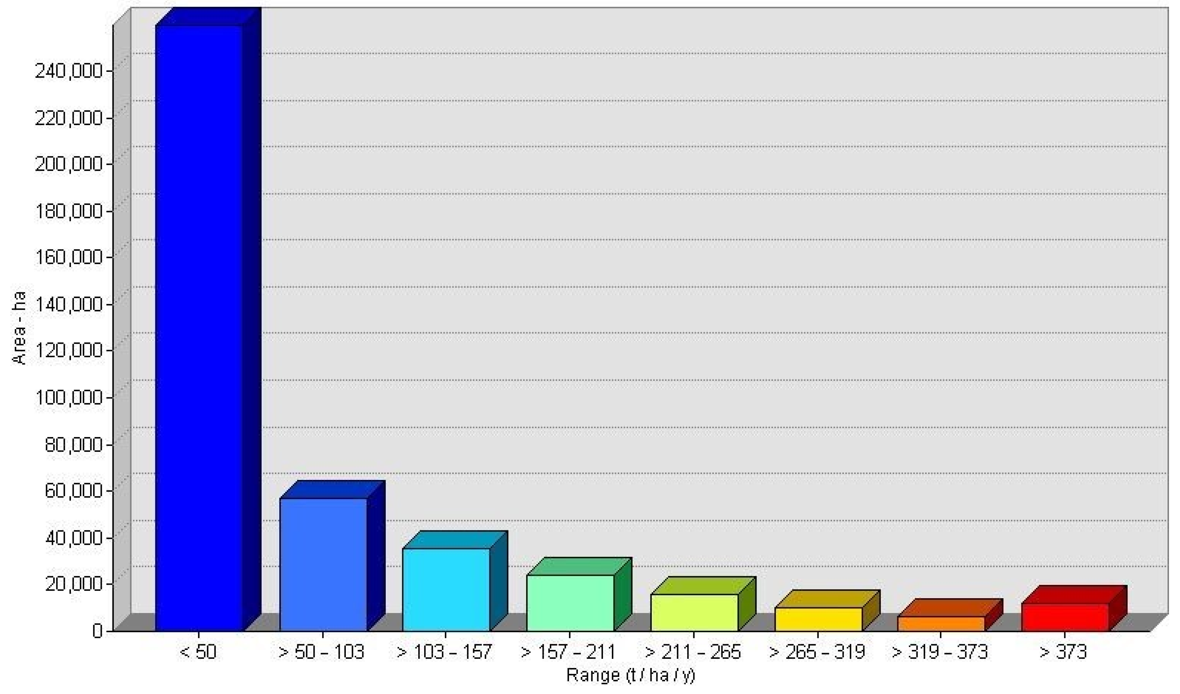
3.4. Soil Erosion (SE)

The results of different factors are combined using the RUSLE equation resulting in an estimation of SE in tons per hectare per year (t-ha⁻¹y⁻¹). The skewed nature of input datasets including LS, OM, and slope tends the SE output in a positively skewed distribution. The generated raster has a mean of 75 t-ha⁻¹y⁻¹ with a high standard deviation of 108.27. The minimum and maximum values of SE are 0 and 799 t-ha⁻¹y⁻¹, respectively.

The SE has spatial variability in low values (SE < 50) t-ha⁻¹y⁻¹ due to the variability of terrain. The low range covers the maximum of the Sanghar catchment. Higher values (SE > 373) t-ha⁻¹y⁻¹ of SE are observed in the central part of the catchment. The clustered high values of SE in the center of the Sanghar catchment is due to the concentration of high values of R, LS, and K-factors and associated heterogeneity in elevations. SE values (211 < SE < 373) t-ha⁻¹y⁻¹ are trending in the adjacent cells of higher SE values. However, the value range of (50 < SE < 211) t-ha⁻¹y⁻¹ covers the rest of the catchment as shown in Figure 8. The generated SE substantiates among the 8 defined ranges, the majority of the area lies in the range (SE < 50) t-ha⁻¹y⁻¹ as shown in Figure 8.

The average value of SE at individual sub-catchment shows strong positive relation with LS-factor. SE values also show a positive relationship with R-factor; however, the relationship is weak as compared to LS-factor. The soil composition also relates to the SE estimates. The average values of SE increase with the increase in percentage sand concentration and decrease with an increase in percentage silt concentration as shown in Figure 9. These two compositions of soil play a significant role in the calculation of the K-factor.

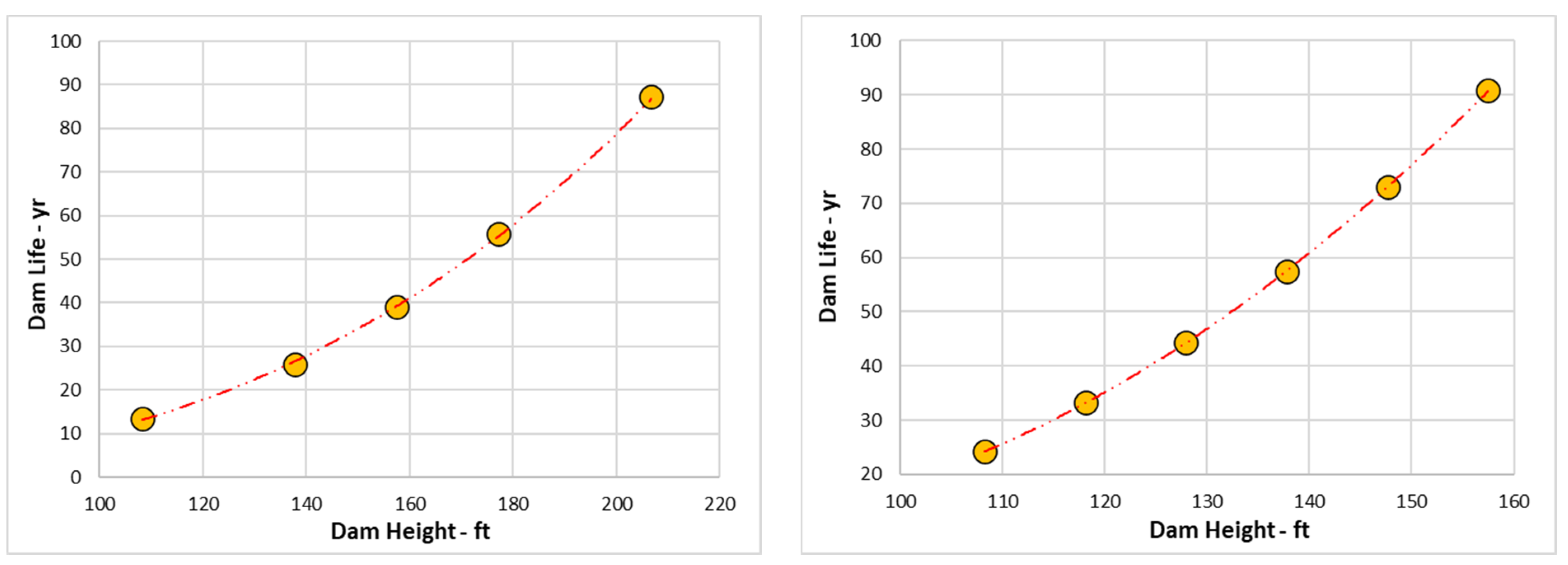
3.5. Sediment Yield and Dam Life

The soil eroded from a catchment due to rainfall is termed as SY. The SY estimates at dam locations solely depend upon the empirical relation of SDR. For both dam locations, the two SDR equations show uncertainties. The SDR relation developed by Swarnkar et al. [64] gives better estimates of SY. The SDR overestimates the SY results for a larger catchment in the area. However, it was observed that the relation behaves well at the sub-catchment level. Based on records of rainfall, the annual average sediment of 298,073 tons and 318,000 tons will feed Dam-A and Dam-B, respectively.

According to the ICOLD [65] classification, a small dam has a height ($2.5 \mathrm{m}<H<15 \mathrm{m})$ and volume of water stored in a reservoir $(H^2\times \sqrt{V}<200 {\mathrm{Mm}}^3)$. However, height restriction is not observed for dam classification in Pakistan, and dams of height $(H>40 \mathrm{m})$ have been constructed as small dams [66]. Based on usual practices in Pakistan lives of selected dams were calculated at 63 m and 48 m height for Dam-A and Dam-B, respectively. The result substantiates approximate lives of 87 and 90 years for Dam-A and Dam-B, respectively, as shown in Figure 10.

4. Discussion

The mountain range of Suleiman with widespread from northeast to southeast of Pakistan is prone to flash floods. The frequent occurrence of low to medium intensity flash floods in the monsoon season makes these catchments more vulnerable as compared to the other parts of Pakistan. The seasonal erratic patterns of rainfall further restrict the usual cultivation of different crops due to the water-scarce nature of the area. The historical cropping level of the hill torrents also indicates that only a small percentage of flood flows during high floods are utilized for agriculture and the remaining flood flows damage canals and canal command area.

Implementation of IMPs (integrated management practices) and BMPs (best management practices) using modern techniques of hydrologic investigations have proven to be a viable method for the management of these areas through dam site suitability and soil loss estimation.

The present study adopts a new methodology for dam site selection using different morphometric datasets including SO, MrVBF, TRI, Slope, CD, VD, and GD. The methodology proves a strong dimension in the dam site selection. The selected parameters/indicators reflect the maximum possible set of rules defined in the literature [3,4,18,67,68] for dam site suitability analysis. The index/indicator as a qualitative approach makes the methodology unique and reduce the user dependency for individual thematic layer generation. Validation of methodology was conducted with an existing dam (Gomal-Zem Dam) in the north of the Suleman mountain range. The adopted methodology identified the Gomal-Zem Dam in a very high suitable class. The designed methodology and selected sites are presented to Secretary and Additional Secretary PID (Punjab Irrigation Department), Pakistan, and found satisfactory. According to [62], both dams are classified in the small dam category. Several studies [3,4,67,68] identified suitable locations for the small dam, check dam, and percolation tank for water harvesting in Pakistan and India. For example, Jamali et al. 2014 [68] present the solution for site suitability for DAM in northern Pakistan using modern techniques of GIS and RS with spatial multi-criterion analysis (SMCA). Singh et al. 2008 [67] identify fourteen suitable sites for check dams using different thematic layers including; LULC, hydrologic soil group, slope, and DEM. The identification of suitable sites followed the guidelines provided by the Integrated Mission for Sustainable Development (IMSD). A latest research has been conducted in Iraq. This research utilized all possible variables including geological formation, soil type, fault line, tectonic line, altitude, slope, rainfall data, water discharge, land use/cover, road network, and material used for dam site selection [69]. Contrarily, very few attempts had been made which utilizes specific indices for dam site suitability analysis. However, the designed methodology grouped certain indices which represent multiple criteria for dam site suitability analysis. The set of indices set well on the varied topography of the areas. The selected indicators cover the maximum set of rules in the literature cited above. The relation between different indicators with the reservoir and dam wall suitability makes the methodology more robust. The selected indicators are generalized and hence could be implemented in any other area.

The efficacy of the designed structure is analyzed by annual average SE estimates. The estimation of SE was necessary because the mountain range of Koh e Suleman is prone to soil erosion due to its varied topography and barren nature of the land cover. The RUSLE equation involves R-rainfall, K-soil erodibility, LS-length slope, C-landcover management, and P-support practice factors to estimate the annual average soil loss of Sanghar torrent. The erratic behavior of rainfall mostly adopting sudden surge from cloud bursts and thunderstorm categorize the episodic nature of streams which remains active in monsoon season (July, August, and September) as shown in Table 2. The high variation in topography and sandy nature increase the soil loss probability in the study area. The SE results using the RUSLE equation shows an average soil loss of 75 t-ha⁻¹y⁻¹. The SY estimates using SDR and SE results show approximately 298,073 tons and 318,000 tons of annual average sediment yield will feed the dam-A and dam-B respectively. The SY results substantiate 87 y and 90 y lives of dam-A and dam-B at a height of 150 ft and 200 ft, respectively. The validation of methodology with limited records of Vidor shows sufficient accuracy of results. The average QOBSERVE and QRUSLE sediment record of Vidor torrent for the monsoon season of 2016 were 7925 t-day⁻¹ and 7455 t-day⁻¹, respectively.

Focusing on the global climate change scenarios, if the frequency of events per year increases dramatically, it will increase the annual soil loss of the Sanghar catchment. The increased SE would decrease the associated dam life. The selected sites have the potential of upraising the dam height up to 385 ft and 325 ft for Dam-A and Dam-B, respectively. The Dam-B with a much higher capacity of 839 million m³ is considered as the main dam for controlling the flash flood peaks. However, Dam-A could be beneficial in series to enhance the life of Dam-B. The strategy is flexible and could be implemented for climate change adaptation schemes. The enriched literature proves the applicability and efficacy of the RUSLE equation. The latest research was conducted by [23] for soil loss estimation using the RUSLE model on the Chitral river catchment in the North of Pakistan. Another study on Rawal Dam catchment in the North of Punjab province, Pakistan, was conducted by [70] and found GIS and RS techniques suitable for SE estimates (R2 = 0.76). Kusimi et al. 2015 [71] studied the effect of uncontrolled land use activities on SE in the Pra River, Ghana using the RUSLE equation. Djoukbala et al. 2018 [72] also evaluate the reliability and effectiveness of the RUSLE equation with the integration of GIS in Wadi El-Ham Algeria and found satisfactory results.

Pakistan is facing a shortage of water for several years, primarily because of the increase in population and mismanagement of accessible water resources. The water war scenario with neighboring countries accentuate the existing drastic nature of water shortage. There is average annual potential of 23 billion m³ in D G Khan’s hill torrent water resources of the country that has not yet been used to its productive potential [73]. To overcome the water shortage of the country climate change adaptation strategies are by far the most suitable practices that has been implemented around the globe. The structural management of flash flood by dam construction also fulfils the crop water requirement (CWR) in the piedmont plains of the area.

5. Conclusions

The study highlights the existing potential of hill torrents in Pakistan. The results promote the use of spate irrigation to improve the cropping intensity of the area. According to Ahmad et al., 2016 [73], the benefit cost ratio of spate irrigation for piedmont plains of D G Khan is higher than canal and ground water. Therefore, the study concludes the efficient utilization of hill torrents for spate irrigation through the construction of small dam that would manage the flash flood water in environmentally friendly way. Further studies should incorporate the CWR calculation which would help in the modelling, demarcation and management of cultural command areas in the downstream of selected dam sites.

The adopted methodology confirms the applicability of IMPs in flash flood and erosion prone areas for the better management of natural hazards. The generated results substantiate effectiveness and reliability of RDSA technique for dam site suitability analysis and RUSLE for annual SE estimates. The study concludes the following testimonials:

• RDSA technique classified total of 269 box-units in very high to very low classes for reservoir and dam wall suitability.
• Qualitative analysis using RDSA technique results in two suitable dam sites (Dam-A and Dam-B) for the management of flash flood water.
• Quantitative analysis reveals maximum possible capacity of 364 million m³ and 838 million m³ of Dam-A and Dam-B, respectively.
• Soil loss estimation using RUSLE method results in average annual SE of 75 t-ha⁻¹y⁻¹.
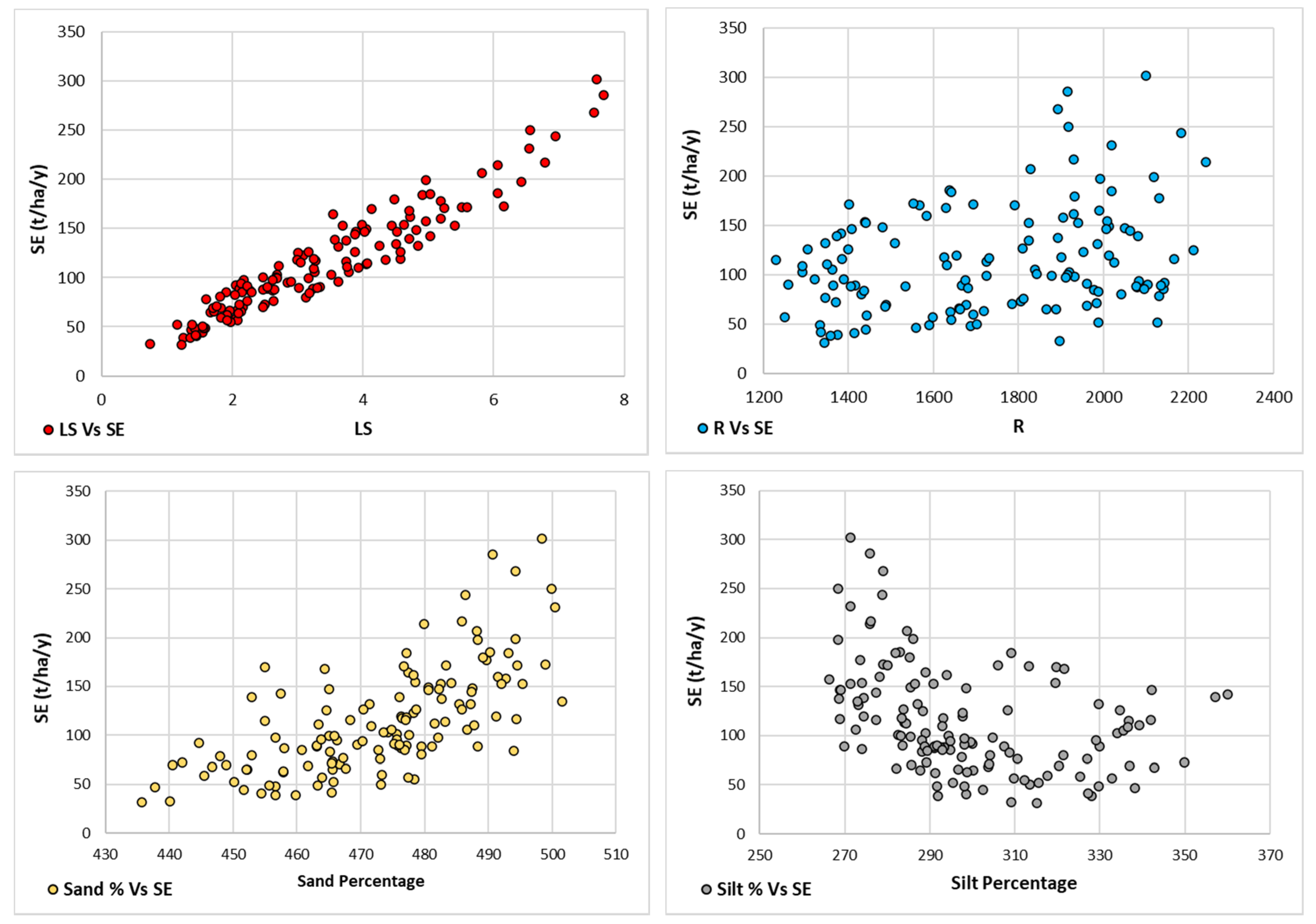
• At sub-catchment level LS, R, percentage of sand and silt concentrations show significant relation with SE.
• SDR and SE based annual average sediment of 298,073 tons and 318,000 tons will feed the Dam-A and Dam-B, respectively
• SY results substantiate approximate lives of 87 and 90 years for Dam-A and Dam-B at height of 150 ft and 200 ft, respectively.

The changing behavior of climate over few decades causes flash flood scenarios more frequent in Pakistan. The proposed sites have the potential to enhance the storage capacity of dams to overcome the long-term forecasted climate change scenarios. The dam wall height of proposed sites can be increased to maximum of 384 ft and 325 ft for Dam-A and Dam-B, respectively.

References

1. Gardiner, E.S.; Hodges, J.D.; Fristoe, T.C. Flood Plain Topography Affects Establishment Success of Direct-Seeded Bottomland Oaks. In Gen. Tech. Rep. SRS–71; US Department of Agriculture, Forest Service, Southern Research Station: Asheville, NC, USA, 2004; pp. 581–585. [Google Scholar]
2. Gioti, E.; Riga, C.; Kalogeropoulos, K.; Chalkias, C. A GIS-based flash flood runoff model using high resolution DEM and meteorological data. Earsel Eproc. 2013, 1, 33–43. [Google Scholar] [CrossRef]
3. Munir, B.A.; Ahmad, S.R.; Hafeez, S. Integrated hazard modeling for simulating torrential stream response to flash flood events. Isprs Int. J. Geo-Inf. 2019, 9, 1. [Google Scholar] [CrossRef] [Green Version]
4. Munir, B.A.; Iqbal, J. Flash flood water management practices in Dera Ghazi Khan City (Pakistan): A remote sensing and GIS prospective. Nat. Hazards 2016, 81, 1303–1321. [Google Scholar] [CrossRef]
5. Norbiato, D.; Borga, M.; Degli Esposti, S.; Gaume, E.; Anquetin, S. Flash flood warning based on rainfall thresholds and soil moisture conditions: An assessment for gauged and ungauged basins. J. Hydrol. 2008, 362, 274–290. [Google Scholar] [CrossRef]
6. Gaume, E.; Bain, V.; Bernardara, P.; Newinger, O.; Barbuc, M.; Bateman, A.; Blaškovičová, L.; Blöschl, G.; Borga, M.; Dumitrescu, A.; et al. A compilation of data on European flash floods. J. Hydrol. 2009, 367, 70–78. [Google Scholar] [CrossRef] [Green Version]
7. Liste, M.; Grifoll, M.; Monbaliu, J. River plume dispersion in response to flash flood events. Application to the Catalan shelf. Cont. Shelf Res. 2014, 87, 96–108. [Google Scholar] [CrossRef]
8. Borga, M.; Boscolo, P.; Zanon, F.; Sangati, M. Hydrometeorological analysis of the 29 August 2003 flash flood in the eastern Italian Alps. J. Hydrometeorol. 2007, 8, 1049–1067. [Google Scholar] [CrossRef]
9. Li, X.; Huang, S.; Sun, T.; Xin, J. Design and Implementation of Flood Monitoring and Assessment System. In Proceedings of the 2011 International Symposium on Image and Data Fusion (ISIDF), Tengchong, China, 9–11 August 2011; pp. 1–3. [Google Scholar]
10. Munir, B.; Imran, H.; Hanif, M. Spatial hazard assessment practices in data poor areas: A participatory approach towards natural disaster management. Int. J. Sci. Basic Appl. Res. IJSBAR 2015, 22, 69–80. Available online: http://gssrr.org/index.php?journal=JournalOfBasicAndApplied&page=article&op=view&path%5B%5D=3799&path%5B%5D=2255 (accessed on 8 July 2020).
11. Petrovic, A. Challenges of torrential flood risk management in Serbia. J. Geogr. Inst. Jovan CVIJIC SASA 2015, 65, 131–143. [Google Scholar] [CrossRef]
12. Veldkamp, T.I.E.; Wada, Y.; Aerts, J.C.J.H.; Döll, P.; Gosling, S.N.; Liu, J.; Masaki, Y.; Oki, T.; Ostberg, S.; Pokhrel, Y.; et al. Water scarcity hotspots travel downstream due to human interventions in the 20th and 21st century. Nat. Commun. 2017, 8, 15697. [Google Scholar] [CrossRef]
13. Li, Z.; Li, W.; Ge, W. Weight analysis of influencing factors of dam break risk consequences. Nat. Hazards Earth Syst. Sci. 2018, 18, 3355–3362. [Google Scholar] [CrossRef] [Green Version]
14. Wu, M.; Ge, W.; Li, Z.; Wu, Z.; Zhang, H.; Li, J.; Pan, Y. Improved set pair analysis and its application to environmental impact evaluation of dam break. Water 2019, 11, 821. [Google Scholar] [CrossRef] [Green Version]
15. Ge, W.; Li, Z.; Liang, R.Y.; Li, W.; Cai, Y. Methodology for establishing risk criteria for dams in developing countries, case study of china. Water Resour. Manag. 2017, 31, 4063–4074. [Google Scholar] [CrossRef]
16. Jozaghi, A.; Alizadeh, B.; Hatami, M.; Flood, I.; Khorrami, M.; Khodaei, N.; Ghasemi Tousi, E. A Comparative Study of the AHP and TOPSIS Techniques for Dam Site Selection Using GIS: A Case Study of Sistan and Baluchestan Province, Iran. Geosciences 2018, 8, 494. [Google Scholar] [CrossRef] [Green Version]
17. Kumar, M.G.; Agarwal, A.K.; Bali, R. Delineation of potential sites for water harvesting structures using remote sensing and GIS. J. Indian Soc. Remote Sens. 2008, 36, 323–334. [Google Scholar] [CrossRef]
18. Al-Ruzouq, R.; Shanableh, A.; Yilmaz, A.G.; Idris, A.E.; Mukherjee, S.; Khalil, M.A.; Gibril, M.B.A. Dam site suitability mapping and analysis using an integrated GIS and machine learning approach. Water 2019, 11, 1880. [Google Scholar] [CrossRef] [Green Version]
19. Sayl, K.N.; Muhammad, N.S. Estimation the physical variables of rainwater harvesting system using integrated GIS-based remote sensing approach. Water Resour. Manag. 2016, 30, 3299–3313. [Google Scholar] [CrossRef]
20. Pandey, A.; Chowdary, V.M.; Mal, B.C.; Dabral, P.P. Remote sensing and GIS for identification of suitabl e sites for soil and water conservation structures. Land Degrad. Dev. 2011, 22, 359–372. [Google Scholar] [CrossRef]
21. Syst, E.; Attribution, C.C.; Weerasinghe, H. Water harvest-and storage-location assessment model using GIS and remote sensing. Hydrol. Earth Syst. Sci. Discuss. 2011, 8, 3353–3381. [Google Scholar]
22. Shit, P.K. Gully Erosion Studies from India and Surrounding Regions; Springer Nature: Berlin/Heidelberg, Germany, 2019. [Google Scholar]
23. Vaezi, A.R. Assessment of soil particle erodibility and sediment trapping using check dams in small semi-arid catchments. Catena 2017, 157, 227–240. [Google Scholar] [CrossRef] [Green Version]
24. Chuenchum, P.; Xu, M.; Tang, W. Estimation of Soil Erosion and Sediment Yield in the Lancang–Mekong River Using the Modified Revised Universal Soil Loss Equation and GIS Techniques. Water 2020, 12, 135. [Google Scholar] [CrossRef] [Green Version]
25. Walling, D.E. Human impact on the sediment loads of Asian rivers. Sediment Problems and Sediment Management in Asian River Basins. IAHS Publ. 2011, 349, 37–51. [Google Scholar]
26. Ashraf, A. Modeling risk of soil erosion in high and medium rainfall zones of Pothwar region, Pakistan. Proc. Pak. Acad. Sci. Pak. Acad. Sci. B Life Environ. Sci. 2017, 54, 67–77. [Google Scholar]
27. Walling, D.E. Measuring sediment yield from river basins. In Soil Erosion Research Methods; Routledge: London, UK, 2017; pp. 39–82. [Google Scholar]
28. Gelagay, H.S.; Minale, A.S. Soil loss estimation using GIS and Remote sensing techniques: A case of Koga watershed, Northwestern Ethiopia. Int. Soil Water Conserv. Res. 2016, 4, 126–136. [Google Scholar] [CrossRef] [Green Version]
29. Atoma, H.; Suryabhagavan, K.; Balakrishnan, M. Soil erosion assessment using RUSLE model and GIS in Huluka watershed, Central Ethiopia. Sustain. Water Resour. Manag. 2020, 6, 12. [Google Scholar]
30. Ullah, S. Geospatial assessment of soil erosion intensity and sediment yield: A case study of Potohar Region, Pakistan. Environ. Earth Sci. 2018, 77, 705. [Google Scholar] [CrossRef]
31. Stephens, T. Manual on Small Earth Dams: A Guide to Siting, Design and Construction (No. 64); Food and Agriculture Organization of the United Nations (FAO): Rome, Italy, 2010. [Google Scholar]
32. Rangsiwanichpong, P.; Kazama, S.; Gunawardhana, L. Assessment of sediment yield in Thailand using revised universal soil loss equation and geographic information system techniques. River Res. Appl. 2018, 34, 1113–1122. [Google Scholar] [CrossRef]
33. Maqsoom, A.; Aslam, B.; Hassan, U.; Kazmi, Z.A.; Sodangi, M.; Tufail, R.F.; Farooq, D. Geospatial assessment of soil erosion intensity and sediment yield using the Revised Universal Soil Loss Equation (RUSLE) model. ISPRS Int. J. Geo-Inf. 2020, 9, 356. [Google Scholar] [CrossRef]
34. Javed, M.Y.; Nadeem, M.; Javed, F. Technical Assistance Consultant’s Report Pakistan: Additional Works for the Preparation of Hill Torrent Management Plan (Financed by TASF) Revised Design/Feasbility Report. 2007. Available online: https://www.adb.org/sites/default/files/project-document/65489/39590-pak-tacr.pdf (accessed on 1 July 2020).
35. Gallant, J.C.; Dowling, T.I. A multiresolution index of valley bottom flatness for mapping depositional areas. Water Resour. Res. 2003, 39, 1347–1359. [Google Scholar] [CrossRef]
36. Riley, S.J.; De Gloria, S.D.; Elliot, R. A Terrain Ruggedness that Quantifies Topographic Heterogeneity. Intermt. J. Sci. 1999, 5, 23–27. [Google Scholar]
37. Conrad, O.; Bechtel, B.; Dietrich, H.; Fischer, E.K.; Gerlitz, L.; Wehberg, J.; Wichmann, V.; Böhner, J. System for Automated Geoscientific Analyses (SAGA) v. 2.1. 4. Geosci. Model Dev. Discuss. 2015, 8, 1991–2007. [Google Scholar] [CrossRef] [Green Version]
38. Khanna, P.N. Indian Practical Civil Engineer’s Handbook, 8th ed.; P.N. Khanna for Engineer’s Publishers: New Delhi, India, 1993. [Google Scholar]
39. Gavade, V.V.; Patil, D.R.R. Site Suitability Analysis for Surface Rainwater Harvesting of Madha Tahsil, Solapur, Maharashtra: A Geoinformatic Approach. 12th ESRI India User. 2011, pp. 1–7. Available online: http://esriindia.com/Events/UC2011_files/WR_UCP0018.pdf (accessed on 10 October 2019).
40. Adhikary, R.G.C.E.; Rai, S.; Shrestha, A. Resource Manual on Flash Flood Risk Management, 3rd ed.; Perlis, A., Ed.; International Center for Integrated Mountain Development: Khatmando, Nepal, 2012; Available online: http://agris.fao.org/agris (accessed on 25 August 2020).
41. FAO. Simple Methods for Aquaculture. 2014. Available online: ftp://ftp.fao.org/FI/CDrom/FAO_Training/FAO_Training/General/x6705e/Index.htm (accessed on 18 February 2020).
42. Ekenberg, L.; Hansson, K.; Danielson, M.; Cars, G. Deliberation Representation Equity: Research Approaches, Tools and Algorithms for Participatory Processes; Open Book Publishers: Cambridge, UK, 2017. [Google Scholar] [CrossRef] [Green Version]
43. Fischer, M.M.; Getis, A. Handbook of Applied Spatial Analysis. In Handbook of Applied Spatial Analysis; Springer: Berlin/Heidelberg, Germany, 2010. [Google Scholar] [CrossRef]
44. Deutsch, K. The Elevation to Area Relationship of Lake Behnke. Undergraduate Journal of Mathematical Modeling: One + Two. 2012. Available online: http://scholarcommons.usf.edu/ujmm/vol4/iss2/5/ (accessed on 6 December 2019).
45. Yahya, A. Surveying: Area and Volumes. Retrieved 9 January 2014. 2002. Available online: http://azlanppd.tripod.com/ (accessed on 2 August 2020).
46. Renard, K.G.; Foster, G.R.; Weesies, G.A.; Porter, J.P. RUSLE: Revised universal soil loss equation. J. Soil Water Conserv. 1991, 46, 30–33. [Google Scholar]
47. Kinnell, P.I. Sediment delivery from hillslopes and the Universal Soil Loss Equation: Some perceptions and misconceptions. Hydrol. Process. Int. J. 2008, 22, 3168–3175. [Google Scholar] [CrossRef]
48. Swarnkar, S.; Malini, A.; Tripathi, S.; Sinha, R. Assessment of uncertainties in soil erosion and sediment yield estimates at ungauged basins: An application to the Garra River basin, India. Hydrol. Earth Syst. Sci. 2018, 22, 2471. [Google Scholar] [CrossRef] [Green Version]
49. Petkovšek, G.; Mikoš, M. Estimating the R factor from daily rainfall data in the sub-Mediterranean climate of southwest Slovenia/Estimation du facteur R à partir de données journalières de pluie dans le climat sub-méditerranéen du Sud-Ouest de la Slovénie. Hydrol. Sci. J. 2004, 49, 5. [Google Scholar] [CrossRef] [Green Version]
50. Richardson, C.W.; Foster, G.R.; Wright, D.A. Estimation of erosion index from daily rainfall amount. Trans. Am. Soc. Agric. Eng. 1983, 26, 153–160. [Google Scholar] [CrossRef]
51. Brown, L.C.; Foster, G.R. Storm erosivity using idealised intensity distributions. Trans. Am. Soc. Agric. Eng. 1987, 30, 293–307. [Google Scholar] [CrossRef]
52. Bagarello, V.; D’Asaro, F. Estimating single storm erosion index. Trans. Am. Soc. Agric. Eng. 1994, 37, 785–791. [Google Scholar] [CrossRef]
53. Wischmeier, W.H.; Smith, D.D. Predicting Rainfall Erosion Losses: A Guide to Conservation Planning (No. 537); Department of Agriculture, Science and Education Administration USDA: Hyattsville, MD, USA, 1978. [Google Scholar]
54. Van der Knijff, J.M.; Jones, R.J.A.; Montanarella, L. Soil Erosion Risk Assessment in Europe, EUR 19044 EN; Office for Official Publications of the European Communities: Luxembourg, 2000; p. 34. [Google Scholar]
55. Nelson, D.W.; Sommers, L.E. Total carbon, organic carbon, and organic matter. Methods Soil Anal. Part 3 Chem. Methods 1996, 5, 961–1010. [Google Scholar]
56. Saxton, K.E.; Rawls, W.J. Soil water characteristic estimates by texture and organic matter for hydrologic solutions. Soil Sci. Soc. Am. J. 2006, 70, 1569–1578. [Google Scholar] [CrossRef] [Green Version]
57. De Boer, F. HiHydroSoil: A High Resolution Soil Map of Hydraulic Properties Version 1.2; Technical Report; FutureWater: Wageningen, The Netherlands, 2016. [Google Scholar]
58. McCool, D.K.; Brown, L.C.; Foster, G.R.; Mutchler, C.K.; Meyer, L.D. Revised slope steepness factor for the Universal Soil Loss Equation. Trans. ASAE 1987, 30, 1387–1396. [Google Scholar] [CrossRef]
59. Renard, K.G.; Foster, G.R.; Weesies, G.A.; McCool, D.K.; Yoder, D.C. Predicting Soil Erosion by Water: A Guide to Conservation Planning with the Revised Universal Soil Loss Equation (RUSLE); Agricultural Handbook 703; U.S. Government Printing Office: Washington, DC, USA, 1997.
60. Desmet, P.J.J.; Govers, G. A GIS procedure for automatically calculating the USLE LS factor on topographically complex landscape units. J. Soil Water Conserv. 1996, 51, 427–433. [Google Scholar]
61. Foster, G.R.; Wischmeier, W. Evaluating irregular slopes for soil loss prediction. Trans. ASAE Gen. Ed. Am. Soc. Agric. Eng. 1974, 17, 305–309. [Google Scholar] [CrossRef]
62. Panagos, P.; Borrelli, P.; Meusburger, K. A new European slope length and steepness factor (LS-Factor) for modeling soil erosion by water. Geosciences 2015, 5, 117–126. [Google Scholar] [CrossRef] [Green Version]
63. FAO. Methodology for Assessing Soil Degradation, Report on the FAO/UNEP Expert Consultation, Rome, 25–27 January 1978; FAO: Rome, Italy, 1978. [Google Scholar]
64. Sharda, V.N.; Ojasvi, P.R. A revised soil erosion budget for India: Role of reservoir sedimentation and land-use protection measures. Earth Surf. Proc. Land. 2016, 41, 2007–2023. [Google Scholar] [CrossRef]
65. Bowles, D.S.; Giuliani, F.L.; Hartford, D.N.; Janssen, J.P.F.M.; McGrath, S.; Poupart, M.; Zielinski, P.A. ICOLD bulletin on dam safety management. IPENZ Proc. Tech. Groups 2007, 33, 2. [Google Scholar]
66. Punjab Irrigation Department. Manual of Irrigation Practice (mip), 2nd ed.; Government of Pakistan: Punjab, Pakistan, 2017. [Google Scholar]
67. Singh, J.P.; Darshdheep, S.; Litoria, P.K. Selection of suitable sites for water harvesting structures in Soankhand watershed, Punjab using remote sensing and Geographical Information System approach-a case study. Indian Soc. Remote Sens. 2008, 37, 21–35. [Google Scholar] [CrossRef]
68. Jamali, I.A.; Mörtberg, U.; Olofsson, B.; Shafique, M. A spatial multi-criteria analysis approach for locating suitable sites for construction of subsurface dams in Northern Pakistan. Water Resour. Manag. 2014, 28, 5157–5174. [Google Scholar] [CrossRef]
69. Noori, A.M.; Pradhan, B.; Ajaj, Q.M. Dam site suitability assessment at the Greater Zab River in northern Iraq using remote sensing data and GIS. J. Hydrol. 2019, 574, 964–979. [Google Scholar] [CrossRef]
70. Samad, N.; Hamid, M.; Muhammad, C.; Saleem, M.; Hamid, Q.; Babar, U.; Farid, M.S. Sediment yield assessment and identification of check dam sites for Rawal Dam catchment. Arab. J. Geosci. 2016, 9, 466. [Google Scholar] [CrossRef]
71. Kusimi, J.M.; Yiran, G.A.; Attua, E.M. Soil erosion and sediment yield modelling in the Pra River Basin of Ghana using the Revised Universal Soil Loss Equation (RUSLE). Ghana J. Geogr. 2015, 7, 38–57. [Google Scholar]
72. Djoukbala, O.; Mazour, M.; Hasbaia, M.; Benselama, O. Estimating of water erosion in semiarid regions using RUSLE equation under GIS environment. Environ. Earth Sci. 2018, 77, 345. [Google Scholar] [CrossRef]
73. Ahmad, M.; Arshad, M.; Cheema, M.; Ahmad, R. Comparison of available water resources for irrigation in Mithawan hill torrent command area of Dera Ghazi Khan, Pakistan. Pak. J. Agric. Sci. 2016, 53, 1. [Google Scholar]
Figure 1. Geographical location of study area.
Ijgi 10 00027 g001
Figure 2. Indicators with suitability relation, Reservoir (left), and Dam Wall (right).
Ijgi 10 00027 g002
Figure 3. Geographical location of proposed dams’ site with stream order.
Ijgi 10 00027 g003
Figure 4. Indicator values for selected sites.
Ijgi 10 00027 g004
Figure 5. Cross-sectional profile of Dam-A (left) and Dam-B (right).
Ijgi 10 00027 g005
Figure 6. EAC curve for Dam-A (left) and Dam-B (right).
Ijgi 10 00027 g006
Figure 7. Soil Erosion (SE) analysis (a); soil type, (b); percentage OM, (c); R-factor, (d); K-factor; (e); LS-factor, and (f); SE.
Ijgi 10 00027 g007
Figure 8. Frequency of SE classes.
Ijgi 10 00027 g008
Figure 9. Relation analysis of RUSLE parameters at the sub-catchment level.
Ijgi 10 00027 g009
Figure 10. Dam life vs. Dam heigh relation; dam-A (left) and dam-B (right).
Ijgi 10 00027 g010