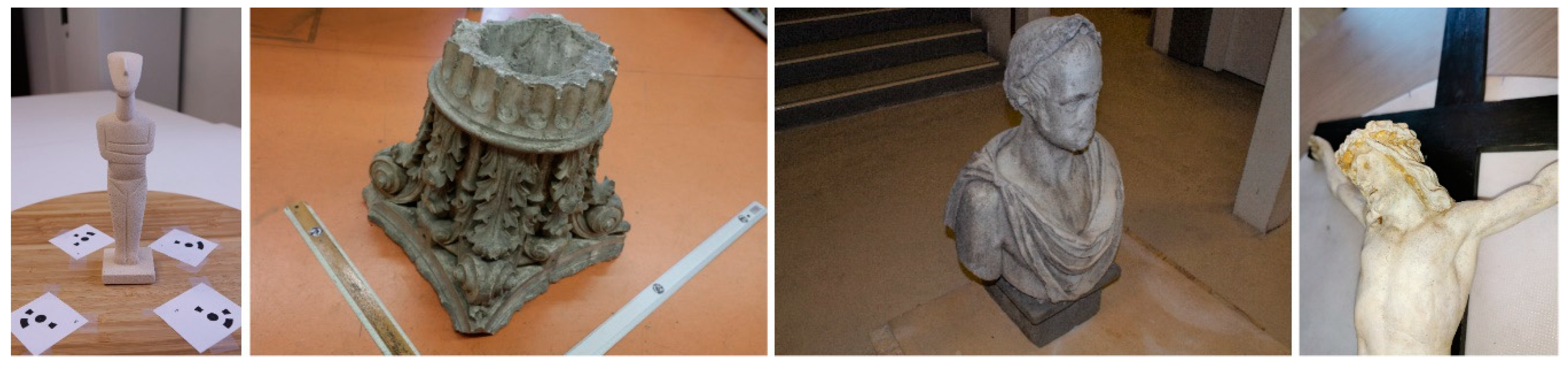
Figure 1.
Case studies (from left to right): Cycladic figurine copy, Roman capital replica, stone bust of Francis Joseph I of Austria, and small sculpture of Christ Crucified.
Figure 1.
Case studies (from left to right): Cycladic figurine copy, Roman capital replica, stone bust of Francis Joseph I of Austria, and small sculpture of Christ Crucified.
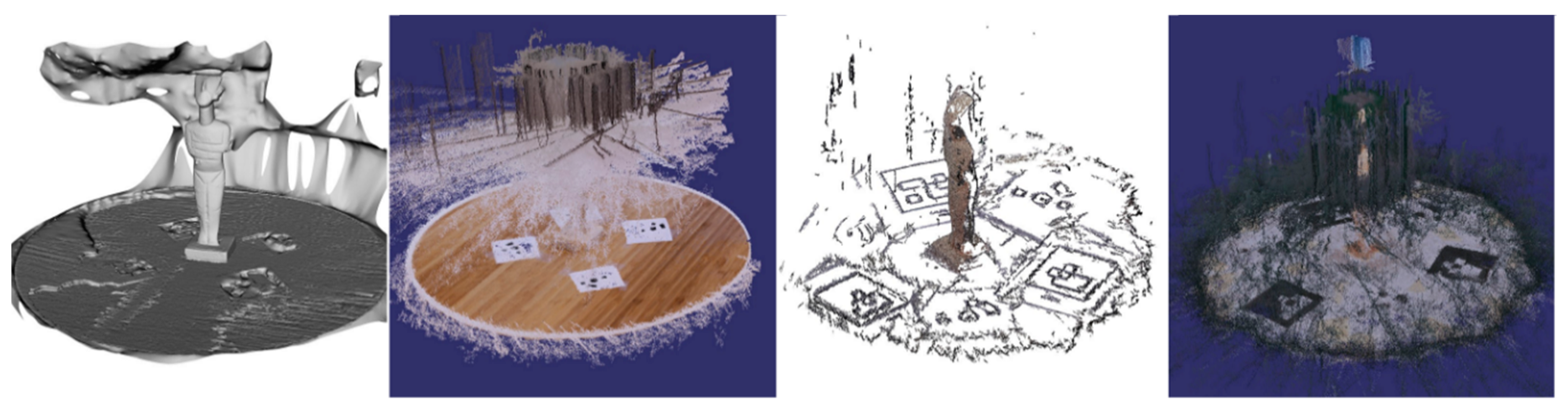
Figure 2.
Examples of partial and noise-containing reconstructions (from left to right): dataset 1 ARP, dataset 1 Regard3D 1.0.0 (R3D), dataset 3 VCM, dataset 3 R3D.
Figure 2.
Examples of partial and noise-containing reconstructions (from left to right): dataset 1 ARP, dataset 1 Regard3D 1.0.0 (R3D), dataset 3 VCM, dataset 3 R3D.
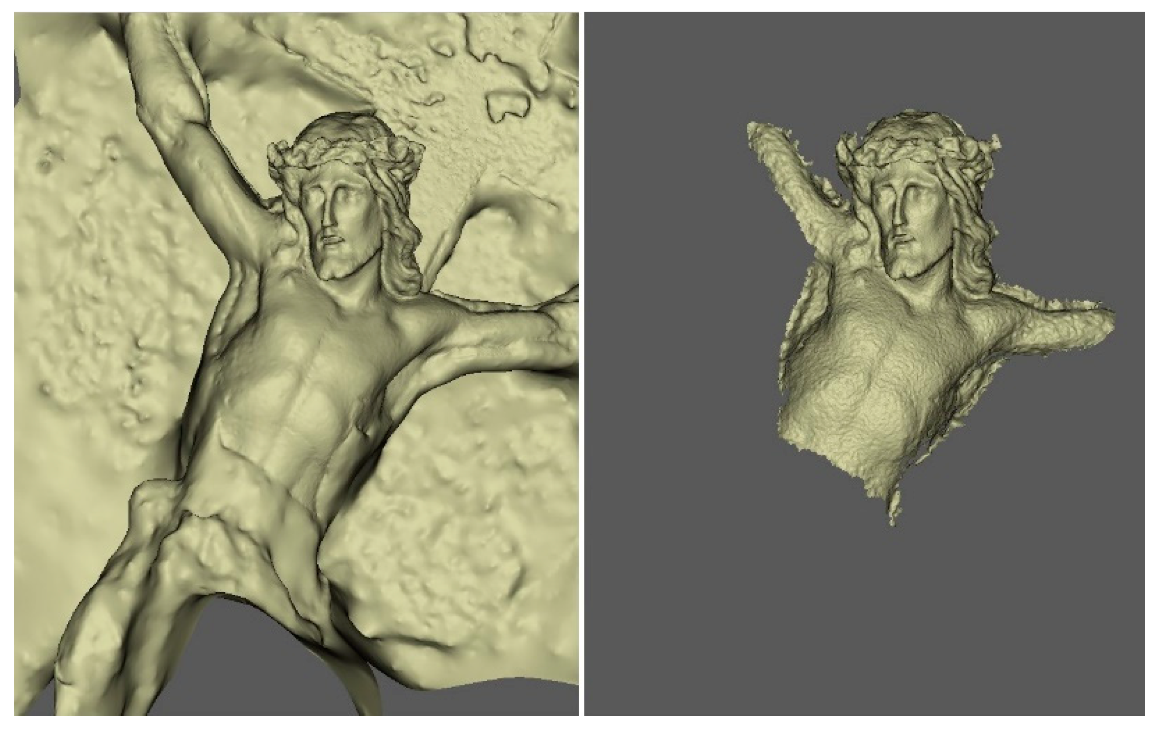
Figure 3.
Partial meshes generated with ARP (left) and FZA (right) from dataset 9.
Figure 3.
Partial meshes generated with ARP (left) and FZA (right) from dataset 9.
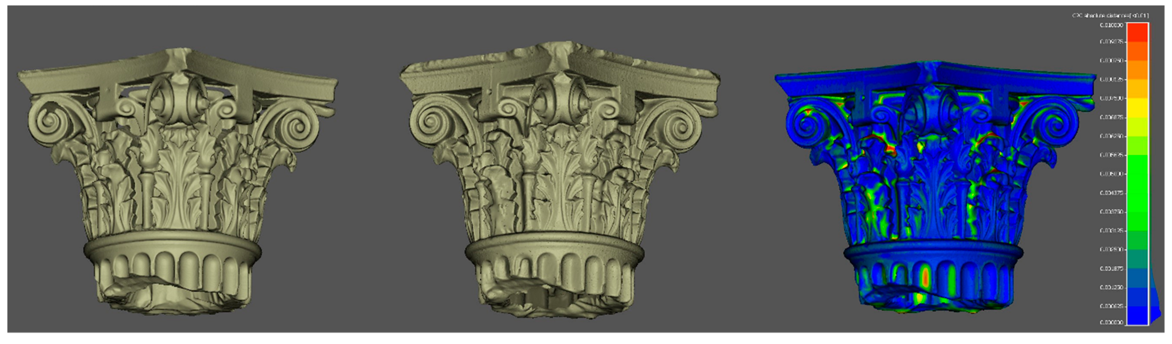
Figure 4.
Scanning results. Untextured Stonex F6 SR mesh (left), untextured FARO Focus 3D X 330 mesh (center) and scalar field mapping of Hausdorff distances; maximum visualized distance: 1 cm.
Figure 4.
Scanning results. Untextured Stonex F6 SR mesh (left), untextured FARO Focus 3D X 330 mesh (center) and scalar field mapping of Hausdorff distances; maximum visualized distance: 1 cm.
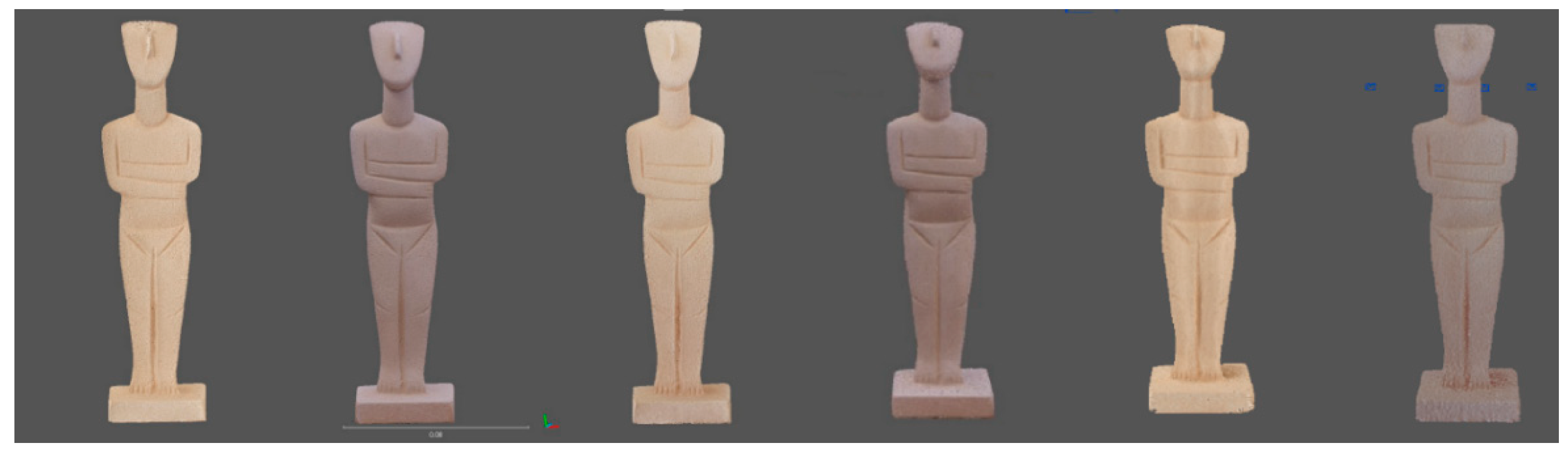
Figure 5.
Textured photogrammetric meshes of the figurine copy, (from left to right) dataset 1 AMP, dataset 1 FZA, dataset 2 AMP, dataset 2 FZA, dataset 3 AMP, dataset 3 FZA.
Figure 5.
Textured photogrammetric meshes of the figurine copy, (from left to right) dataset 1 AMP, dataset 1 FZA, dataset 2 AMP, dataset 2 FZA, dataset 3 AMP, dataset 3 FZA.
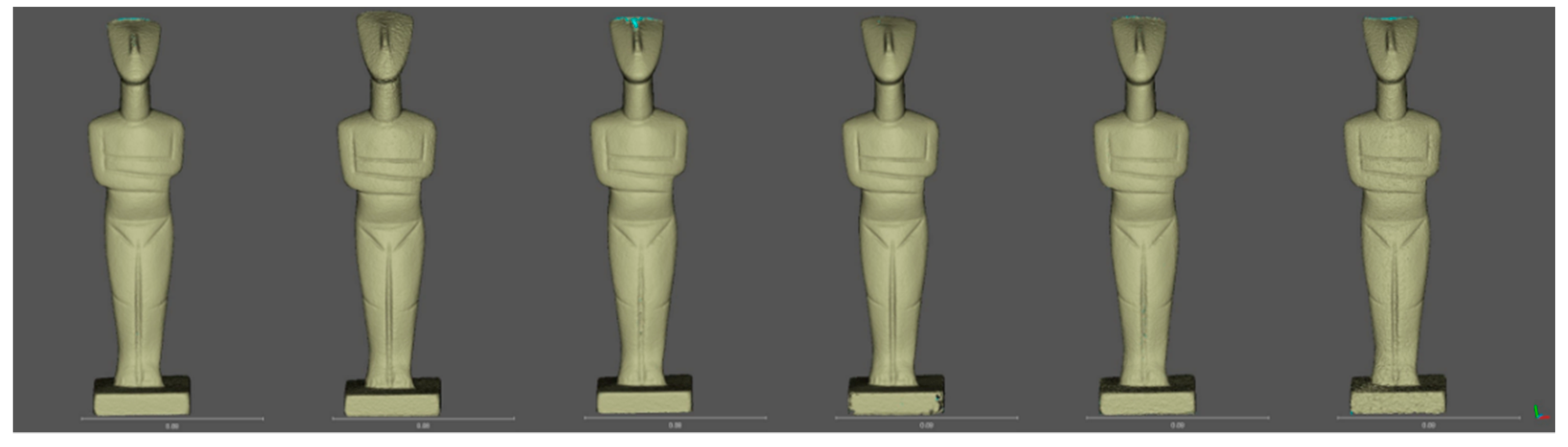
Figure 6.
Untextured photogrammetric meshes of the figurine copy, (from left to right) dataset 1 AMP, dataset 1 FZA, dataset 2 AMP, dataset 2 FZA, dataset 3 AMP, dataset 3 FZA.
Figure 6.
Untextured photogrammetric meshes of the figurine copy, (from left to right) dataset 1 AMP, dataset 1 FZA, dataset 2 AMP, dataset 2 FZA, dataset 3 AMP, dataset 3 FZA.
Figure 7.
Untextured photogrammetric meshes from dataset 4, (from left to right) AMP, FZA, P4D, ARP, VCM.
Figure 7.
Untextured photogrammetric meshes from dataset 4, (from left to right) AMP, FZA, P4D, ARP, VCM.
Figure 8.
Scalar field mapping of Hausdorff distances for dataset 4 photogrammetric results. Deviation between the ARP mesh and the AMP mesh (left), deviation between the ARP mesh and the FZA mesh (center), deviation between the ARP and the P4D mesh (right); maximum visualized distance: 1 cm.
Figure 8.
Scalar field mapping of Hausdorff distances for dataset 4 photogrammetric results. Deviation between the ARP mesh and the AMP mesh (left), deviation between the ARP mesh and the FZA mesh (center), deviation between the ARP and the P4D mesh (right); maximum visualized distance: 1 cm.
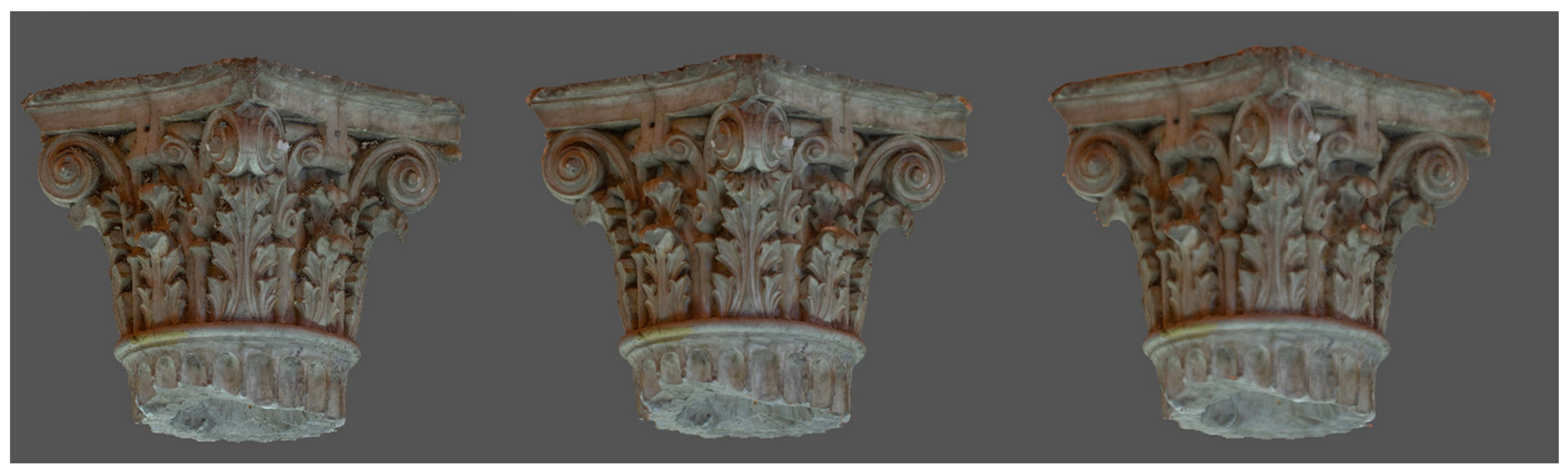
Figure 9.
Textured photogrammetric meshes of the capital replica from dataset 5 (from left to right): AMP, VCM, R3D.
Figure 9.
Textured photogrammetric meshes of the capital replica from dataset 5 (from left to right): AMP, VCM, R3D.
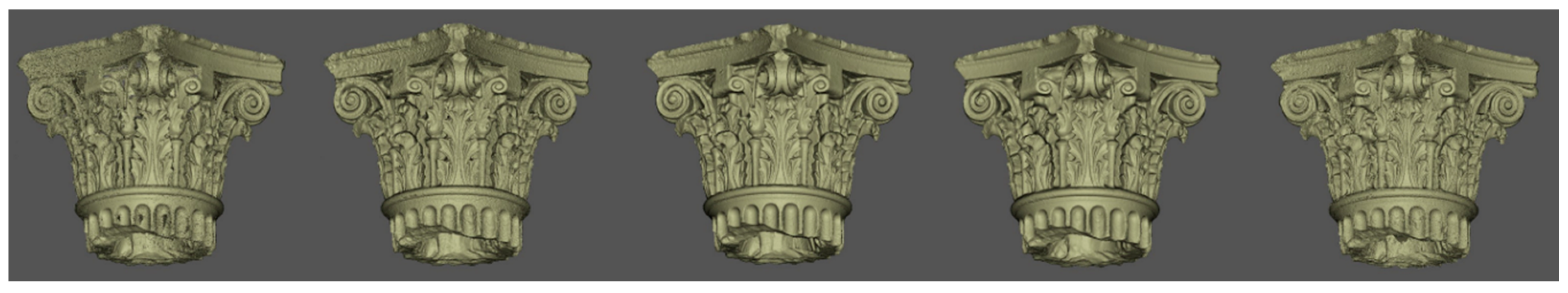
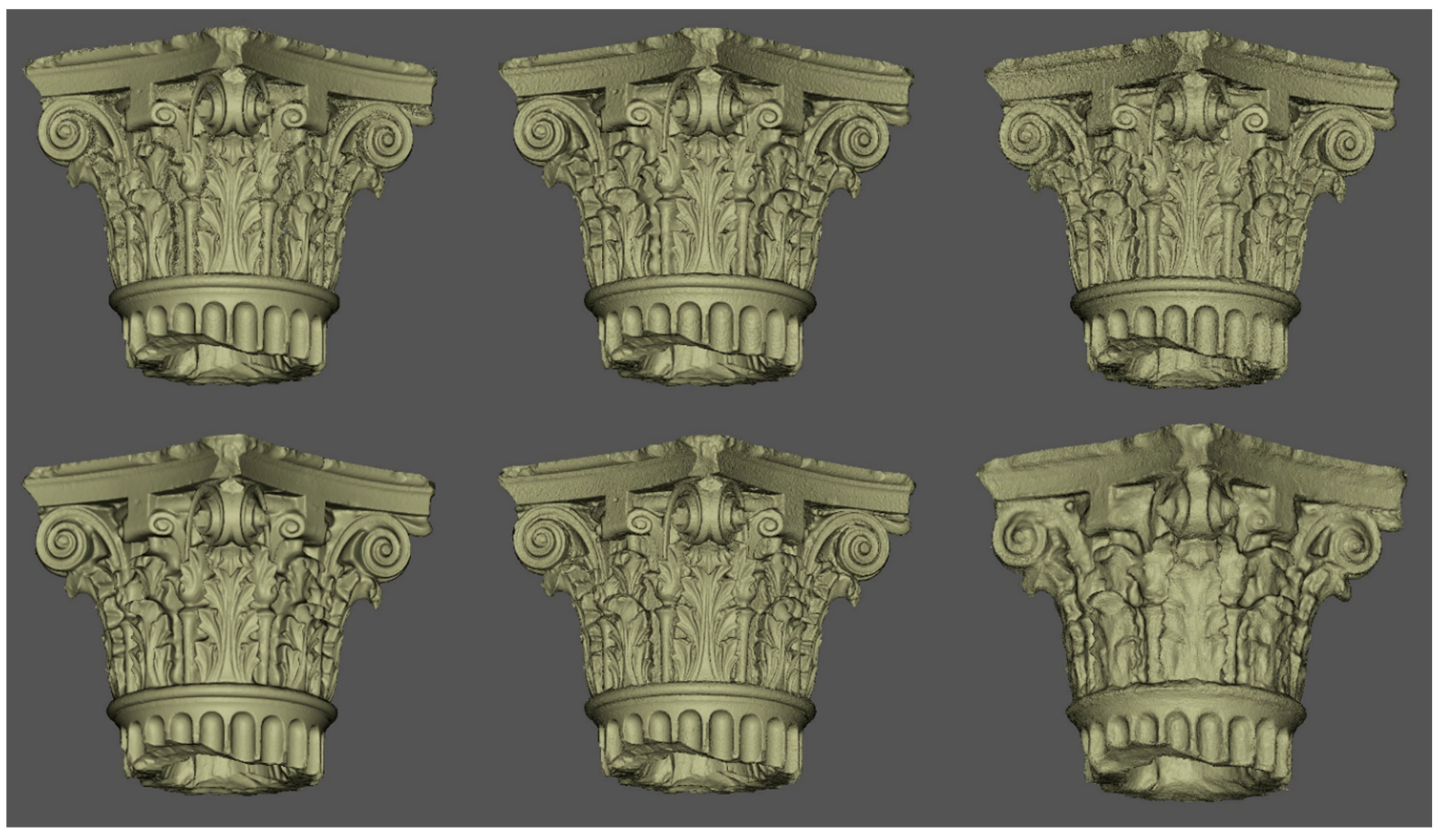
Figure 10.
Untextured photogrammetric meshes of the capital replica from dataset 5, (from left to right, and from top to bottom): AMP, FZA, P4D, ARP, VCM, R3D.
Figure 10.
Untextured photogrammetric meshes of the capital replica from dataset 5, (from left to right, and from top to bottom): AMP, FZA, P4D, ARP, VCM, R3D.
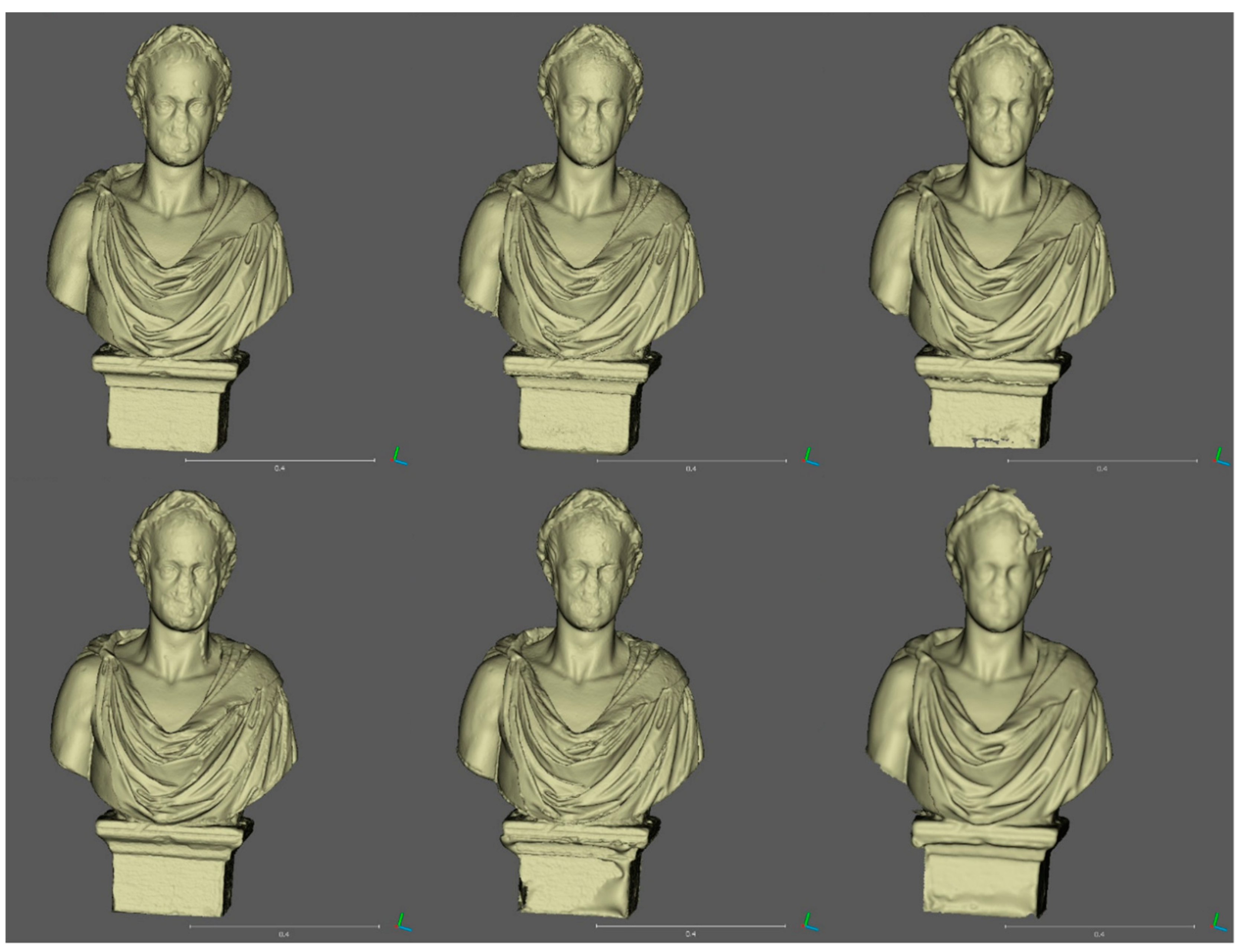
Figure 11.
Untextured meshes of the stone bust from dataset 6 (from left to right, and from top to bottom): F6 SR, AMP, FZA, ARP, VCM, R3D.
Figure 11.
Untextured meshes of the stone bust from dataset 6 (from left to right, and from top to bottom): F6 SR, AMP, FZA, ARP, VCM, R3D.
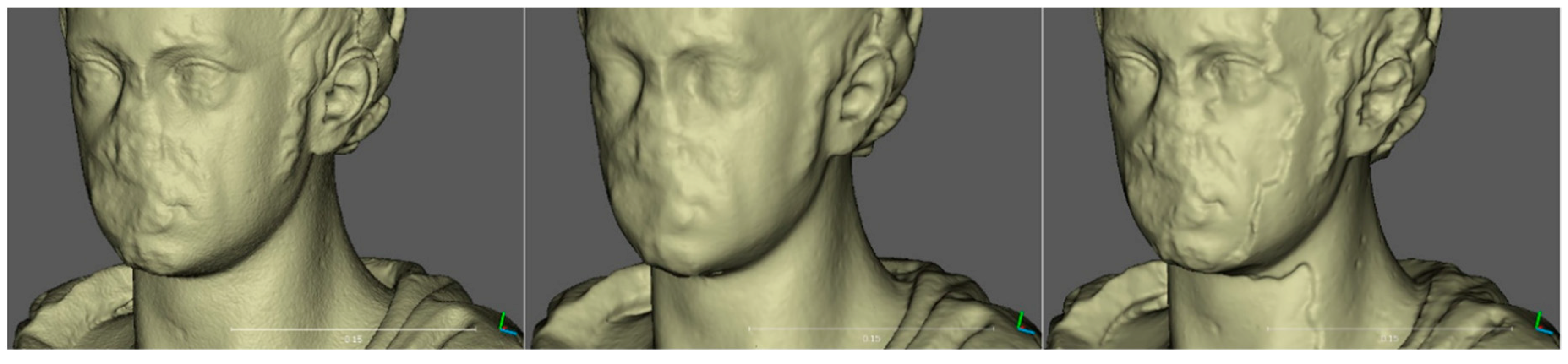
Figure 12.
Detail from the untextured photogrammetric meshes of the stone bust from dataset 6 (from left to right): F6 SR, FZA, ARP.
Figure 12.
Detail from the untextured photogrammetric meshes of the stone bust from dataset 6 (from left to right): F6 SR, FZA, ARP.
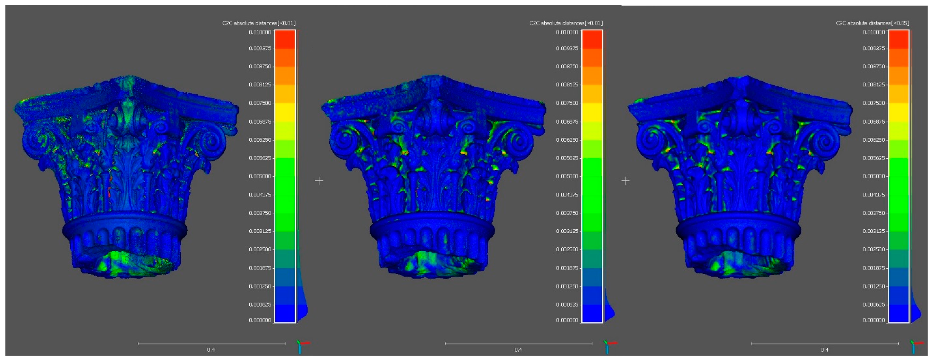
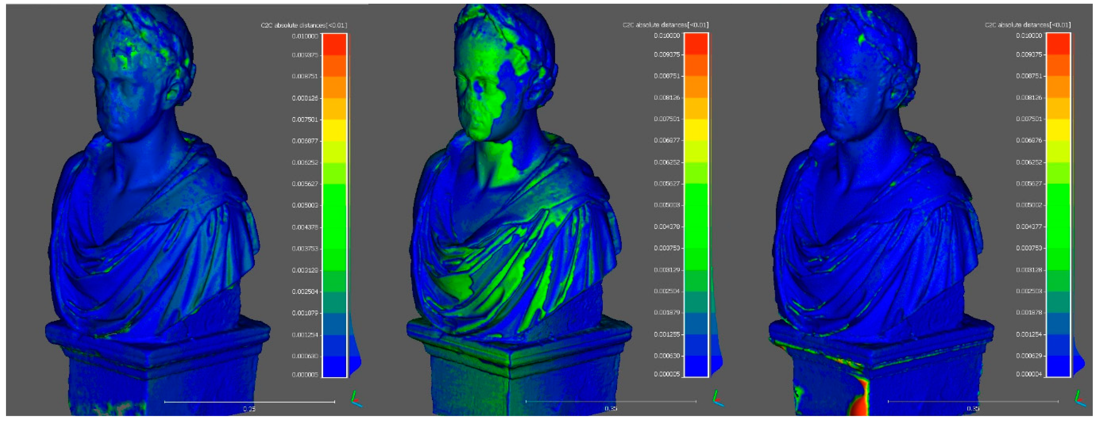
Figure 13.
Scalar field mapping of Hausdorff distances for dataset 6 photogrammetric results. Deviation between the AMP mesh and the FZA mesh (left), deviation between the AMP mesh and the ARP mesh (center), deviation between the AMP and the VCM mesh (right); maximum visualized distance: 1 cm.
Figure 13.
Scalar field mapping of Hausdorff distances for dataset 6 photogrammetric results. Deviation between the AMP mesh and the FZA mesh (left), deviation between the AMP mesh and the ARP mesh (center), deviation between the AMP and the VCM mesh (right); maximum visualized distance: 1 cm.
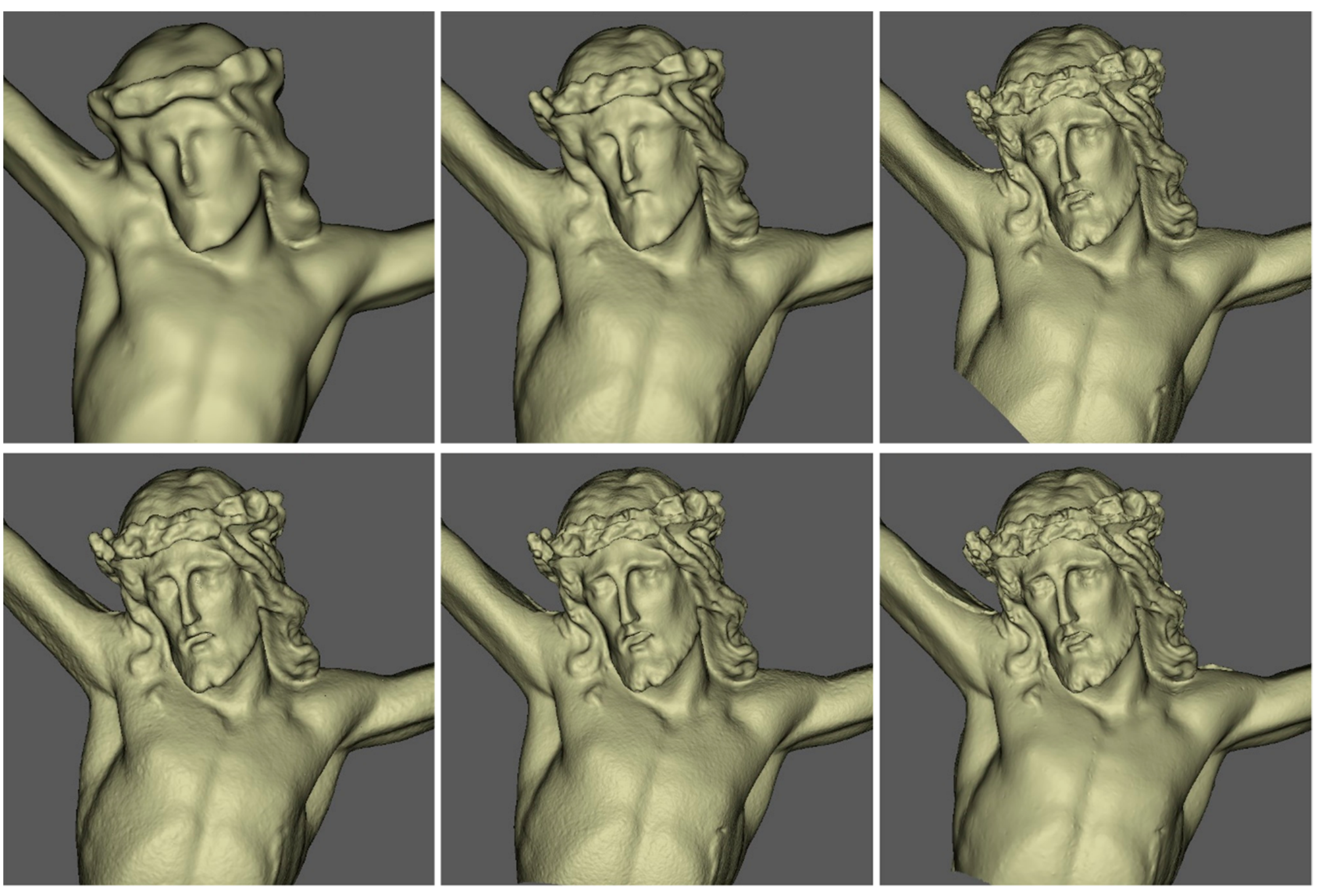
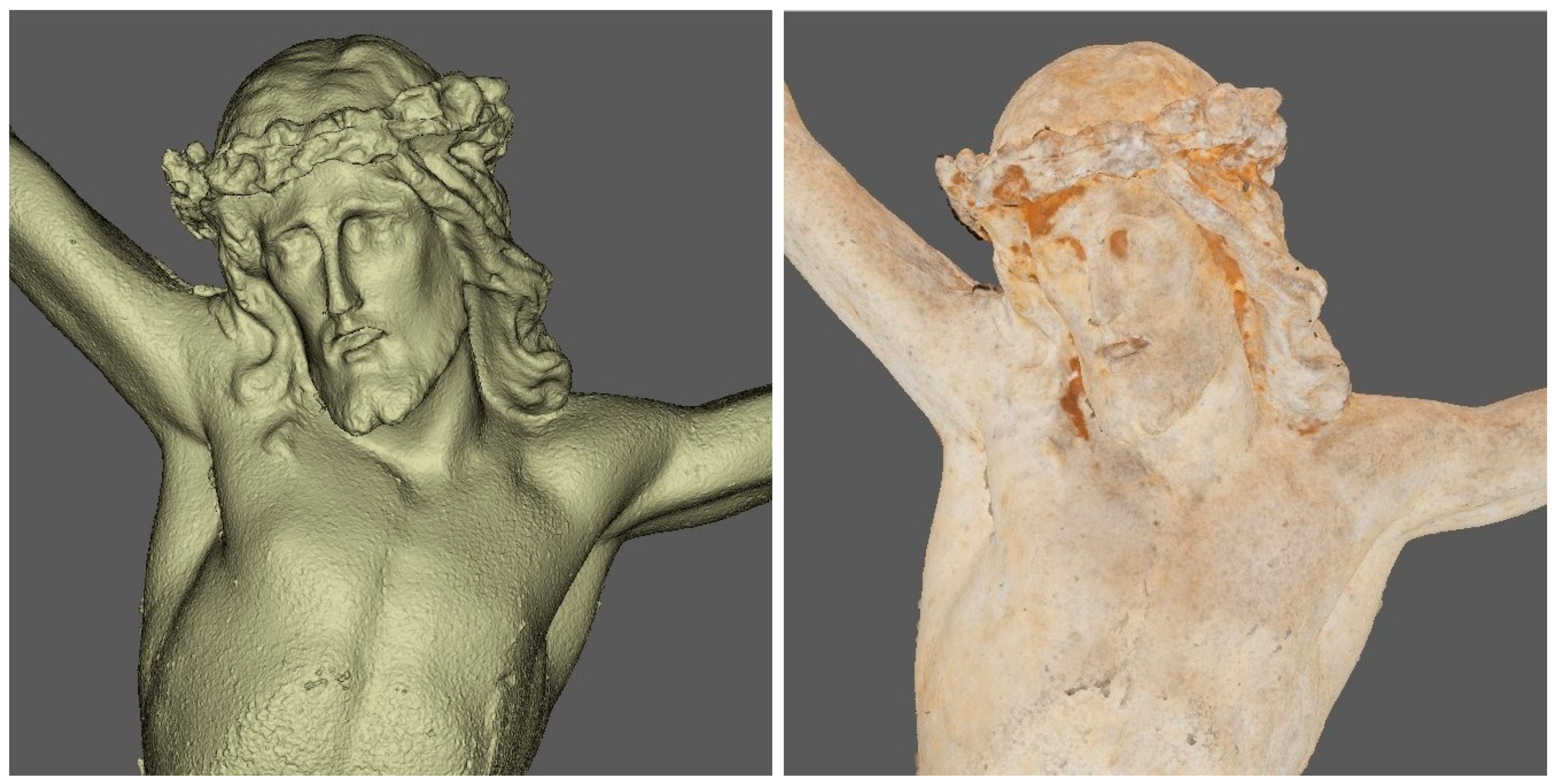
Figure 14.
Untextured meshes of the small sculpture, (from left to right, and from top to bottom): F6 SR, AMP–dataset 7, AMP–dataset 8, FZA–dataset 7, FZA–dataset 8, and ARP–dataset 8.
Figure 14.
Untextured meshes of the small sculpture, (from left to right, and from top to bottom): F6 SR, AMP–dataset 7, AMP–dataset 8, FZA–dataset 7, FZA–dataset 8, and ARP–dataset 8.
Figure 15.
VCM-produced mesh from dataset 9 (smartphone camera).
Figure 15.
VCM-produced mesh from dataset 9 (smartphone camera).
Figure 16.
Scalar field mapping of Hausdorff distances between dataset 6 photogrammetric results and scanning results. Deviation between the F6 SR mesh and the AMP mesh (upper left), deviation between the F6 SR mesh and the FZA mesh (upper right), deviation between the F6 SR mesh and the ARP mesh (lower left), deviation between the F6 SR and the VCM mesh (lower right); maximum visualized distance: 1 cm.
Table 1.
Specifications of the employed imaging sensors.
Table 2.
Characteristics of imagery datasets.
Table 2.
Characteristics of imagery datasets.
| Dataset | Object | Camera
Model | Mega-
Pixels | f (mm) | Distance (m) | No. of Images | f-Stop | Exposure (s) | ISO |
|---|
| 1 | Figurine copy | EOS 5DS R | 52 | 24 | 0.25 | 50 | f/7.1 | 1/20 | 200 |
| 2 | Figurine copy | EOS 1200D | 18 | 18 | 0.20 | 50 | f/8 | 1/20 | 200 |
| 3 | Figurine copy | Exmor RS IMX650 | 40 | 5.6 | 0.25 | 50 | f/8 | 1/20 | 200 |
| 4 | Capital replica | EOS 5DS R | 52 | 35 | 0.88 * | 50 | f/7.1 | 1/40 | 200 |
| 5 | Capital replica | EOS 1200D | 18 | 18 | 0.69 * | 50 | f/8 | 1/40 | 200 |
| 6 | Stone bust | EOS 1200D | 18 | 18 | 0.90 * | 50 | f/16 | 1/60 | 100 |
| 7 | Small sculpture | EOS 1200D | 18 | 18 | 0.38 | 142 | f/16 | 1/15 | 100 |
| 8 | Small sculpture | EOS 1200D | 18 | 55 | 0.27 | 60 | f/16 | 1/15 | 100 |
| 9 | Small sculpture | Exmor RS IMX650 | 40 | 5.6 | 0.12 | 60 | f/1.8 | 1/50 | 100 |
Table 3.
Processing parameters of image-based photogrammetric modeling.
Table 3.
Processing parameters of image-based photogrammetric modeling.
| Reconstruction Step | Parameter | Value |
|---|
| Feature detection and matching alignment | Key point density | High (50K) |
| Tie point density | High (50K) |
| Pair preselection | Higher matches |
| Camera model fitting | Refine |
Dense
matching | Point density | High |
| Depth filtering | Moderate |
Mesh
generation | Max number of faces | 5M (10M for capital replica) |
| Surface interpolation | Limited |
Texture
generation | Texture size | 8192 × 8192 pixels |
| Color balancing | Disabled |
Table 4.
Photogrammetric results, datasets 1–3.
Table 4.
Photogrammetric results, datasets 1–3.
| | | Dataset 1 | Dataset 2 | Dataset 3 |
|---|
| | Software | AMP | FZA | AMP | FZA | AMP | FZA |
|---|
| Sparse Cloud | Images Aligned | 50 | 50 | 50 | 50 | 50 | 42 |
| Matching time (hh:mm:ss) | 00:00:40 | 00:02:48 | 00:00:18 | 00:01:40 | 00:00:41 | 00:05:34 |
| Alignment time (hh:mm:ss) | 00:00:19 | 00:01:11 | 00:00:06 | 00:00:20 | 00:00:10 | 00:00:34 |
| Tie points (1000 points) | 98 | 24 | 29 | 19 | 77 | 27 |
| Projections (1000 points) | 321 | 136 | 92 | 91 | 212 | 118 |
| Adjustment error (pixels) | 0.49 | 0.79 | 0.54 | 0.46 | 0.65 | 0.72 |
| Resolution (mm/pixel) | 0.05 | 0.05 | 0.06 | 0.06 | 0.04 | 0.04 |
| Dense Cloud | Processing time (hh:mm:ss) | 00:10:31 | 01:16:39 | 00:04:31 | 00:24:03 | 00:09:09 | 00:46:40 |
| Point count (1000 points) | 1832 | 591 | 1169 | 370 | 2414 | 3920 |
| Triangle Mesh | Processing time (hh:mm:ss) | 00:00:21 | 00:00:08 | 00:00:16 | 00:00:47 | 00:00:30 | 00:00:10 |
| Faces (1000 triangles) | 4482 | 1168 | 2846 | 737 | 5000 | 1551 |
| Vertices (1000 points) | 2246 | 589 | 1427 | 369 | 2514 | 783 |
| Texture | Processing time (hh:mm:ss) | 00:04:07 | 00:04:01 | 00:02:46 | 00:01:25 | 00:05:49 | 00:02:32 |
| | Total time (hh:mm:ss) | 00:15:58 | 01:24:47 | 00:07:57 | 00:28:15 | 00:16:19 | 00:55:30 |
Table 5.
Photogrammetric results, datasets 4 and 5.
Table 5.
Photogrammetric results, datasets 4 and 5.
| | | Dataset 4 | Dataset 5 |
|---|
| | Software | AMP | FZA | P4D | AMP | FZA | P4D |
|---|
| Sparse Cloud | Images Aligned | 50 | 50 | 50 | 50 | 50 | 50 |
| Matching time (hh:mm:ss) | 00:01:05 | 00:10:14 | 0:00:51 | 00:01:04 | 00:09:23 | 00:00:49 |
| Alignment time (hh:mm:ss) | 00:00:33 | 00:01:02 | 0:02:53 | 00:00:21 | 00:00:27 | 0:01:50 |
| Tie points (1000 points) | 197 | 78 | 1262 | 102 | 52 | 547 |
| Projections (1000 points) | 535 | 361 | 2697 | 258 | 247 | 1126 |
| Adjustment error (pixels) | 0.98 | 1.44 | 0.17 | 0.69 | 0.94 | 0.11 |
| Resolution (mm/pixel) | 0.08 | 0.09 | 0.08 | 0.16 | 0.16 | 0.16 |
| Dense Cloud | Processing time (hh:mm:ss) | 00:23:15 | 01:44:35 | 00:11:35 | 00:07:51 | 00:31:01 | 00:03:15 |
| Point count (1000) | 43,611 | 2168 | 12,032 | 10,941 | 1811 | 3742 |
| Manual denoizing | no | no | no | no | no | no |
| Triangle Mesh | Processing time (hh:mm:ss) | 00:36:40 | 00:00:27 | 00:07:20 | 00:03:44 | 00:00:21 | 00:00:44 |
| Faces (1000 triangles) | 10,000 | 4245 | 10,000 | 9995 | 3587 | 10,000 |
| Vertices (1000 points) | 7739 | 2935 | 7445 | 5507 | 2293 | 6773 |
| Texture | Processing time (hh:mm:ss) | 00:36:16 | 00:07:00 | 00:35:40 | 00:11:35 | 00:04:36 | 00:10:02 |
| | Total time (hh:mm:ss) | 01:37:49 | 02:03:18 | 0:58:19 | 00:24:35 | 00:45:48 | 00:16:40 |
Table 6.
Photogrammetric results, dataset 6.
Table 6.
Photogrammetric results, dataset 6.
| | | Dataset 6 |
|---|
| | Software | VCM | R3D | ARP | AMP | FZA |
|---|
| Sparse Cloud | Images aligned | 50 | 48 | 50 | 50 | 50 |
| Matching time (hh:mm:ss) | 00:02:19 | 00:03:36 | | 00:00:36 | 00:00:59 |
| Alignment time (hh:mm:ss) | 00:01:03 | 00:00:30 | | 00:00:13 | 00:17:34 |
| Tie points (1000 points) | 23 | 143 | | 59 | 48 |
| Projections (1000 points) | 75 | 498 | | 156 | 205 |
| Adjustment error (pixels) | 1.30 | 0.17 | | 0.52 | 0.60 |
| Dense Cloud | Processing time (hh:mm:ss) | 00:11:39 | 00:23:01 | | 00:05:37 | 00:22:22 |
| Point count (1000 points) | 1582 | 11,786 | | 9880 | 2666 |
| Triangle Mesh | Processing time (hh:mm:ss) | 00:06:05 | 00:01:02 | | 00:06:31 | 00:02:01 |
| Faces (1000 triangles) | 1451 | 252 | 1003 | 5000 | 3737 |
| Vertices (1000 points) | 726 | 127 | 1848 | 2500 | 1873 |
| Texture | Processing time (hh:mm:ss) | 00:01:52 | 00:00:48 | | 00:03:10 | 00:03:54 |
| | Total time (hh:mm:ss) | 0:22:58 | 0:28:57 | | 0:16:07 | 0:46:50 |
Table 7.
Photogrammetric results, datasets 7–9.
Table 7.
Photogrammetric results, datasets 7–9.
| | | Dataset 7 | Dataset 8 | Dataset 9 |
|---|
| | Software | AMP | FZA | AMP | FZA | VCM | AMP | FZA |
|---|
| Sparse Cloud | Images aligned | 142 | 69 | 60 | 60 | 60 | 60 | 23 |
| Matching time (hh:mm:ss) | 00:01:05 | 00:03:40 | 00:01:55 | 0:01:39 | 00:01:22 | 00:01:38 | 0:02:58 |
| Alignment time (hh:mm:ss) | 0:00:24 | 00:09:05 | 00:01:19 | 00:46:48 | 00:01:28 | 00:00:55 | 0:28:02 |
| Tie points (1000 points) | 89 | 36 | 420 | 132 | 54 | 88 | 34 |
| Projections (1000 points) | 273 | 154 | 1270 | 803 | 253 | 242 | 127 |
| Adjustment error (pixels) | 0.52 | 0.52 | 0.35 | 0.47 | 1.02 | 1.15 | 1.43 |
| Resolution (mm/pixel) | 0.09 | 0.09 | 0.02 | 0.02 | 0.02 | 0.02 | 0.2 |
| Dense Cloud | Processing time (hh:mm:ss) | 00:23:10 | 00:55:20 | 00:14:27 | 00:42:16 | 00:15:43 | 00:25:30 | 00:25:06 |
| Point count (1000 points) | 2058 | 4211 | 9980 | 3958 | 1764 | 11,325 | 1720 |
| Triangle Mesh | Processing time (hh:mm:ss) | 00:01:23 | 00:02:30 | 00:02:58 | 00:03:34 | 00:06:03 | 00:05:32 | 00:01:13 |
| Faces (1000 triangles) | 4846 | 4605 | 5000 | 4839 | 3864 | 5000 | 2061 |
| Vertices (1000 points) | 2424 | 2312 | 2563 | 2500 | 1935 | 2504 | 1055 |
| Texture | Processing time (hh:mm:ss) | 00:09:25 | 00:18:25 | 00:03:59 | 00:09:50 | 00:09:47 | 00:04:09 | 00:02:51 |
| | Total time (hh:mm:ss) | 0:35:27 | 1:29:00 | 0:24:38 | 1:44:07 | 0:34:23 | 0:37:44 | 1:00:10 |
Table 8.
Specifications of the employed scanners.
Table 9.
Scanning results, capital replica.
Table 9.
Scanning results, capital replica.
| | STONEX F6 SR | FARO Focus3D X 330 | FARO Freestyle |
|---|
| Acquisition duration (mm:ss) | 02:16 | 90:56 | 10:40 |
| Registration duration (mm:ss) | 05:08 | 14:35 | --- |
| Denoising duration (mm:ss) | 24:15 | 2:26 | 00:02 |
| Meshing duration (mm:ss) | 01:23 | 04:01 | 01:27 |
| Cloud points (1000 points) | 20,928 | 1289 | 435 |
| Mesh triangles (1000 triangles) | 6350 | 6488 | 1951 |
Table 10.
Hausdorff distances between the photogrammetric models for the figurine copy case study—datasets 1–3 (distances in mm).
Table 10.
Hausdorff distances between the photogrammetric models for the figurine copy case study—datasets 1–3 (distances in mm).
| | Dataset 2 AMP | Dataset 3 AMP | Dataset 1 FZA | Dataset 2 FZA | Dataset 3 FZA |
|---|
| Dataset 1 AMP | 0.15 | 0.11 | 0.17 | 0.14 | 0.21 | 0.29 | 0.16 | 0.15 | 0.19 | 0.18 |
| Dataset 2 AMP | | | 0.19 | 0.16 | 0.23 | 0.28 | 0.21 | 0.18 | 0.18 | 0.14 |
| Dataset 3 AMP | | | | | 0.18 | 0.17 | 0.17 | 0.14 | 0.15 | 0.10 |
| Dataset 1 FZA | | | | | | | 0.20 | 0.20 | 0.17 | 0.16 |
| Dataset 2 FZA | | | | | | | | | 0.16 | 0.10 |
| | Mean abs. | Std. dev | Mean abs. | Std. dev | Mean abs. | Std. dev | Mean abs. | Std. dev | Mean abs. | Std. dev |
Table 11.
Hausdorff distances between the photogrammetric models for the capital replica case study—dataset 4 (distances in mm).
Table 11.
Hausdorff distances between the photogrammetric models for the capital replica case study—dataset 4 (distances in mm).
| | FZA | P4D | ARP | VCM | R3D |
|---|
| AMP | 0.66 | 0.45 | 0.75 | 1.30 | 0.76 | 0.59 | 0.69 | 0.54 | 0.80 | 0.57 |
| FZA | | | 0.80 | 1.50 | 0.72 | 0.78 | 0.72 | 0.71 | 0.79 | 0.68 |
| P4D | | | | | 0.95 | 2.14 | 0.94 | 1.06 | 0.96 | 1.07 |
| ARP | | | | | | | 0.80 | 0.67 | 0.82 | 0.64 |
| VCM | | | | | | | | | 0.60 | 0.59 |
| | Mean abs. | Std. dev | Mean abs. | Std. dev | Mean abs. | Std. dev | Mean abs. | Std. dev | Mean abs. | Std. dev |
Table 12.
Hausdorff distances between the photogrammetric models for the capital replica case study—dataset 5 (distances in mm).
Table 12.
Hausdorff distances between the photogrammetric models for the capital replica case study—dataset 5 (distances in mm).
| | FZA | P4D | ARP | VCM | R3D |
|---|
| AMP | 0.60 | 0.45 | 0.68 | 0.81 | 0.72 | 0.99 | 0.50 | 0.50 | 5.45 | 3.33 |
| FZA | | | 0.94 | 1.06 | 1.04 | 1.23 | 0.73 | 0.68 | 5.37 | 3.23 |
| P4D | | | | | 1.07 | 1.51 | 0.90 | 0.95 | 5.48 | 3.22 |
| ARP | | | | | | | 1.05 | 1.51 | 5.55 | 3.23 |
| VCM | | | | | | | | | 5.37 | 3.26 |
| | Mean abs. | Std. dev | Mean abs. | Std. dev | Mean abs. | Std. dev | Mean abs. | Std. dev | Mean abs. | Std. dev |
Table 13.
Hausdorff distances between the photogrammetric models for the stone bust case study—dataset 6 (distances in mm).
Table 13.
Hausdorff distances between the photogrammetric models for the stone bust case study—dataset 6 (distances in mm).
| | FZA | ARP | VCM | R3D |
|---|
| AMP | 0.82 | 0.58 | 1.28 | 0.89 | 0.69 | 0.82 | 1.03 | 1.31 |
| FZA | | | 1.21 | 1.31 | 1.00 | 1.15 | 1.11 | 1.37 |
| ARP | | | | | 1.44 | 1.19 | 1.68 | 1.5 |
| VCM | | | | | | | 1.21 | 1.36 |
| | Mean abs. | Std. dev | Mean abs. | Std. dev | Mean abs. | Std. dev | Mean abs. | Std. dev |
Table 14.
Hausdorff distances between photogrammetric models for the small sculpture case study—datasets 7–9 (distances in mm).
Table 14.
Hausdorff distances between photogrammetric models for the small sculpture case study—datasets 7–9 (distances in mm).
| | AMP–Dataset 7 | FZA–Dataset 7 | AMP–Dataset 8 | VCM–Dataset 9 |
|---|
| AMP–Dataset 8 | 0.70 | 1.45 | 0.81 | 1.53 | 0.24 | 0.48 | 0.28 | 0.86 |
| | mean abs. | std. dev. | mean abs. | std. dev. | mean abs. | std. dev. | mean abs. | std. dev. |
Table 15.
Hausdorff distances between the 3D scanning and photogrammetric models from dataset 4 (distances in mm).
Table 15.
Hausdorff distances between the 3D scanning and photogrammetric models from dataset 4 (distances in mm).
| | AMP | FZA | P4D | ARP | VCM | R3D |
|---|
| 3D X 330 | 0.84 | 2.18 | 1.01 | 1.57 | 1.32 | 2.14 | 1.17 | 1.69 | 1.21 | 1.79 | 1.01 | 1.04 |
| F6 SR | 1.72 | 1.75 | 1.23 | 1.40 | 1.23 | 1.43 | 1.48 | 1.61 | 1.21 | 1.39 | 1.17 | 1.35 |
| | Mean abs. | Std. dev | Mean abs. | Std. dev | Mean abs. | Std. dev | Mean abs. | Std. dev | Mean abs. | Std. dev | Mean abs. | Std. dev |
Table 16.
Hausdorff distances between 3D scanning and photogrammetric models from dataset 5 (distances in mm).
Table 16.
Hausdorff distances between 3D scanning and photogrammetric models from dataset 5 (distances in mm).
| | AMP | FZA | P4D | ARP | VCM | R3D |
|---|
| 3D X 330 | 1.46 | 1.96 | 1.29 | 1.90 | 1.37 | 2.16 | 1.42 | 2.04 | 1.25 | 2.09 | 5.75 | 3.30 |
| F6 SR | 1.53 | 2.16 | 1.54 | 1.41 | 1.22 | 1.43 | 1.51 | 1.69 | 1.31 | 1.44 | 6.22 | 3.33 |
| | Mean abs. | Std. dev | Mean abs. | Std. dev | Mean abs. | Std. dev | Mean abs. | Std. dev | Mean abs. | Std. dev | Mean abs. | Std. dev |
Table 17.
Hausdorff distances between the 3D scanning and photogrammetric models from dataset 6 (distances in mm).
Table 17.
Hausdorff distances between the 3D scanning and photogrammetric models from dataset 6 (distances in mm).
| | AMP | FZA | ARP | VCM | R3D |
|---|
| F6 SR | 0.63 | 0.73 | 0.66 | 0.65 | 1.22 | 1.00 | 0.75 | 0.92 | 1.11 | 1.38 |
| | Mean abs. | Std. dev | Mean abs. | Std. dev | Mean abs. | Std. dev | Mean abs. | Std. dev | Mean abs. | Std. dev |


