An Analysis of Joint Assembly Geometric Errors Affecting End-Effector for Six-Axis Robots

Abstract

This paper presents an analysis of the geometric errors of joint assembly that affect the end-effector for a six-axis industrial robot. The errors were composed of 30 parameters that come from the Geometric Dimensioning and Tolerancing (GD&T) design, which is not the normal way to describe them. Three types of manufacturing tolerancing—perpendicularity, parallelism and position—were introduced and investigated. These errors were measured by the laser tracker. The measurement data were calculated with an analysis of the circle fitting method. The kinematic model and error model based on a combination of translations methods were used. The experiment was carried out in order to calculate the tolerancing of geometric error. Then, the positions of the end-effector in the actual measurement from laser tracker and exact performance were compared. The discrepancy was compensated by offline programming. As a result, the position errors were reduced by 90%.

1. Introduction

Industrial robots are widely used in manufacturing and in processes such as welding, milling, grinding and drilling. The demand for industrial robots with better repeatability and accuracy has been growing. The accuracy of the robot is not important, as long as the robot end-effector poses are manually taught. However, in offline programming, accuracy becomes important, since positions are defined in a virtual space with respect to a coordinated system. Thus, the accuracy of the robot is becoming a more important measurement to indicate the accuracy and precision of an industrial robot. The actual position coordinate of a robot’s tool center point deviates from the nominal value due to the inherent geometric errors. The inaccuracies can be caused by many sources. They include deformation, thermal, controller and structure. Much research into robot positioning accuracy has been carried out. The geometric or kinematic errors may affect the positioning accuracy of a robot. The imperfect geometric, alignments and dimensions of machine components are sources. In the current study, the focus is on structural errors [1,2,3,4,5,6].

Many researches have been conducted in kinematic error analysis, error model derivation and calibration of robotics and machine tools [7,8,9,10,11]. A lot of research has studied the positioning error, and claimed that the geometric error is the most important factor with respect to the positioning error of the robotics [12,13,14,15]. Yuanfan et al. [15] have studied an error compensation method with error similarity analysis to improve the absolute positional accuracy of industrial robots. The ordinary kriging method is used to calculate positional errors. Shaowai et al. [16] presents an integrated geometric error modeling, identification and compensation method for machine tools. The geometric error parameter is based on a laser interferometer and ball bar. Nguyen et al. [17] have proposed a method of full pose measurement of the robot end-effector for calibration. The method is based on an analysis of the features of a set of target points on a circle trajectory. Zhu et al. [4] have proposed a positioning error compensation on two-dimensional manifold that reduces the dimensionality of the workspace. OH [11] presents the data measured during the circle contouring movement of the robot end-effector to analyze the robot’s orientation error. The geometric error calibration and compensation have been widely studied to improve the robot accuracy. Geometric Dimensioning and Tolerancing (GD&T) is another factor of geometric errors. The nominal geometrics of a robot as determined in the design drawing can rely on the development of the nominal kinematic function. It is often used in the central controller for robots of the same model without taking the variation in the assembled robots into account [18]. The variation owes much to the tolerances allowed in the manufacturing of the robot components. For the nominal to fit better in all the robots of the same model, the tolerances specified in the design drawing have to be tightened. This is a potentially expensive approach to improving positioning accuracy. The development of kinematic models is important in evaluating the performance of a robot system and in improving its positioning accuracy. An error model is also important during the robotic calibration. The correct identification of the kinematic error model can serve to increase the effectiveness of robot positioning accuracy. Error models have been developed based on homogeneous matrices and Jacobian matrices [19].

There are many measurement tools that are used in machine tools and robot calibration, such as laser interferometer, laser ball bar, ball-column, laser tracker, optical CMM and visual system [20,21,22,23]. An et al. [20] use a laser tracker calibration and compensation of machine tool volumetric error. Cao et al. [21] have studied a method to reduce and compensate the position error of robot using machine vision combined with a neural network. Albert et al. [22] present a technique used to find the 29 error parameters of an ABB IRB 1600 robot that best fit the measures acquired with a laser tracker. Error compensation, which uses a specific mathematical way to model the error in the industry machining process, such as positioning, thermal field, force, etc. [4], is a promising method to improve the machining precision.

This study proposes measurement tolerances, which are a factor of the joint assembly geometric errors, which affect end-effector for six-axis robots. The method in this study is designed to measure the pose and path error combination of the robot that is composed by measuring with 7-line directions, which provide a more precise analysis of the Geometric Dimensioning and Tolerancing effect than the conventional kinematic calibration of industrial robots due to the conventional kinematic calibration, which can measure the position error. Normally, the conventional kinematic errors are measured and evaluated the position errors that combine all the factors of the end-effector, while the proposed methods analyze the geometric errors of each joint, and can be separate joint errors compensated by both off-line programming and mechanical adjustment methods. The following sections of this paper are organized as follows: Section 2 discusses a kinematic model and geometric error model based on a combination of translations methods. This model is implemented in a KUKA KR5 six-axis robot. The total amount of geometric errors is measured in the first experiment by a laser tracker. The second experiment measures and compares the robot end-effector position between the normal kinematic model and the proposed kinematic model. The third experiment is carried out in order to validate the performance of geometric errors induced by error compensation. Geometric errors are compensated in offline programming in the test. The Laser tracker measures the uncompensated and compensated results of seven direction position errors. The experiment is described in detail in Section 3. The results of the experimental verification are shown in Section 4, and finally the conclusions are drawn in Section 5.

2. Mathematic Error Model of Industrial Robots

2.1. Robot Kinematic Model

There are several methods to describe robot kinematics. The most widely used presentation is the DH parameter [13,18,23,24]. However, this study selected a combination of translation methods for transformation kinematics that modify the DH method [25]. The DH method was used to represent a simple robot model, but this paper analyzes the positioning error at the end-effector caused by the GD&T of each robot’s joints, which have to be added to the transformation of errors in each joint into robot kinematics. Therefore, the transformation kinematic with errors cannot use the DH method directly. The combination of translations consists of translations and rotations about a current frame axis. Any transformation can be resolved into a set of translations and rotations in order to accomplish what is needed. This order is very important, and if the order of two successive transformations is changed, the result may be different. All transformation changes are the location of the current frame relative to the new reference frame. The new location of the frame relative to the fixed reference frame can be defined by the translations $Trans(d_x,d_y,d_z)$, the rotation about $xRot(x,\gamma )$, the rotation about $yRot(y,\beta )$ and the rotation about $zRot(z,\alpha )$. The transformation between two link frames is defined in terms of the combination of translations as

$$P_i=Trans(d_x,d_y,d_z)Rot(x,\gamma )Rot(y,\beta )Rot(z,\alpha )$$

(1)

where P_i is the rotation frame relative to the reference frame. A homogeneous transformation matrix, which refers to the transformation of the ith link relative to (i + 1)th link frame as

$$A_{i+1}=Rot(z,\theta )P_i=\left(\begin{array}{cc}{R}_{i+1}& T_{i+1}\\ 0& 1\end{array}\right)$$

(2)

where $Rot(z,{\theta }_i)$ is a joint angle. The $R_i$ is a 3 × 3 rotation matrix, and $T_i$ is a 3 × 1 translation matrix. For a 6-axis robot, a seven reference frame $P_i$ (i ranging from 0 to 6) are defined, and the forward kinematic model is defined as

$$T=A_1{A}_2{A}_3{A}_4{A}_5{A}_6{A}_7$$

(3)

This method can be applied to any robot model; a robot KUKA KR5 (Figure 1) has been considered in this implementation. A nominal dimension of the robot is shown in

Table 1. A nominal dimension of the KUKA KR5.

Link	Rotation (°)	Translation (mm)	θ (°)
1	About x 180	Along z 225	−
2	About x 90	Along x 180, y 120, z −175	θ1
3	About z −90	Along x 600, z −15	θ2
4	About x 90	Along x 120, y 413.5, z 135	θ3
5	About x −90	Along z −206.5	θ4
6	About x 90	Along y 108.8	θ5
7	About y 180	Along z −6.2	θ6

.

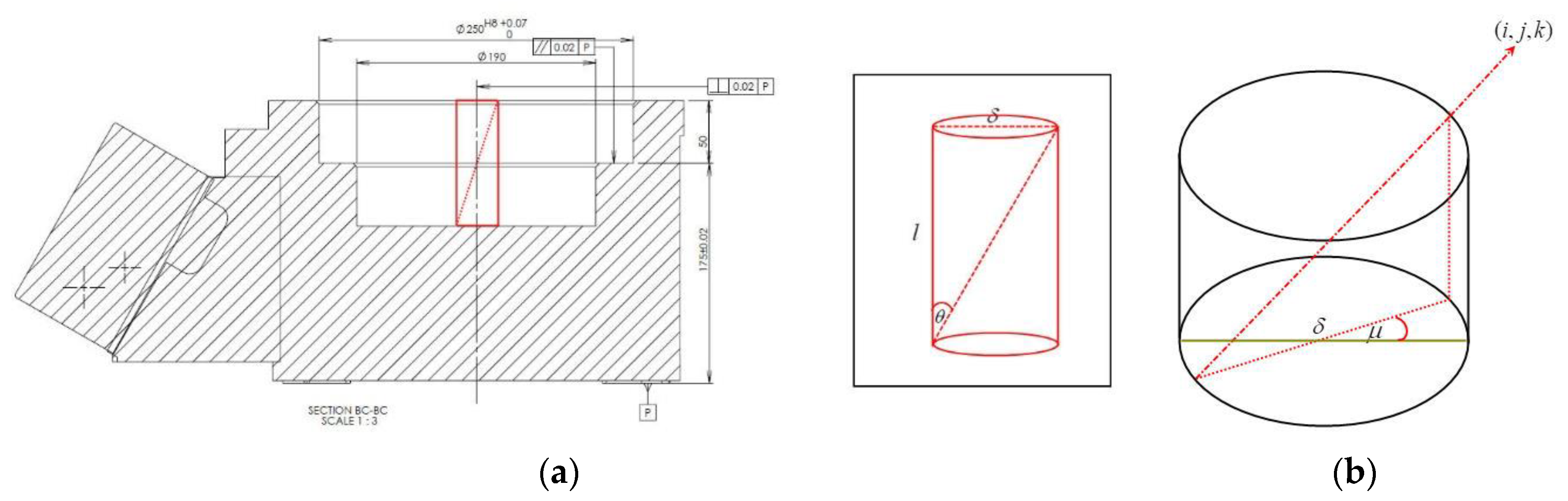
2.2. Geometric Error Model

The accuracy of the machine tool and robot is affected by many possible error sources. The types of error can be distinguished into static errors and random errors. Static errors are those whose numerical value and sign are constant for each robot, such as geometric errors. Random errors are those whose numerical value or sign change unpredictably. At each robot, the exact magnitude and direction of random errors cannot be uniquely determined, such as the backlash of a motor gearbox [18].

The geometric errors are static errors. There are many sources of geometric errors that may affect the accuracy of end-effect positioning. Kinematic errors are errors due to imperfect geometric, alignment and dimensions of machine components. Geometric Dimensioning and Tolerancing (GD&T) is another factor of error. Tolerancing is considered an error. In this study, these errors include perpendicularity, parallelism and position. Rotation transformation is the result of perpendicularity and parallelism. Translation Transformation is the result of the position.

The Geometric Transformation of tolerancing changes the geometric properties of a robot. As a result, the frames defined at the robot joints are displaced from a nominal location. In Figure 2, frame $P_i^n$ is shown in a nominal location and frame $P_i^r$ is reallocated due to error.

The position and orientation of frame $P_i^r$ with respect to frame $P_i^n$ that is represented by a 4 × 4 homogenous matrix $E_i$ are the same as the combination of translations of kinematic transformation. The error transformation matrix can be described by

$$E_i=T_e\times R_e$$

(4)

where $R_e$ is the rotation error part of matrix $E_i$ is the result of the product of two consecutive rotations $e_{\beta }$ and $e_{\gamma }$ about the Y and X axis, respectively. The subscript $\beta$ represents pitch and $\gamma$ represents yaw. The part of the roll (rotation about Z axis) has been canceled by the robot mastering process. $T_e$ is the translation error part of matrix $E_i$, which is composed of the three coordinates $e_x$, $e_y$ and $e_z$ of $O_i^n$ to $O_i^r$. The five parameters $e_{\beta }$, $e_{\gamma }$, $e_x$, $e_y$ and $e_z$ are called geometric errors parameters which can be written as

$$E_i=Trans(e_{xi},e_{yi},e_{zi})\times Rot(x,e_{\gamma i})\times Rot(y,e_{\beta i})$$

(5)

For a 6-axis robot, there are 30 geometric errors, which can be written in matrix form as

$$E_i=\left(\begin{array}{cccc}\cos (e_{\beta i})& 0& \sin (e_{\beta i})& e_{xi}\\ \sin (e_{\beta i})sin(e_{\gamma i})& \cos (e_{\gamma i})& -\cos (e_{\beta i})sin(e_{\gamma i})& e_{yi}\\ -\sin (e_{\beta i})cos(e_{\gamma i})& \sin (e_{\gamma i})& \cos (e_{\beta i})\cos (e_{\gamma i})& e_{zi}\\ 0& 0& 0& 1\end{array}\right)$$

(6)

When the geometric errors are considered in the 6-axis robot model, a homogeneous transformation matrix with error is defined in Equation (6), and the forward kinematic model with error is the same as in Equation (3)

$$T_{w/e}=A_1{E}_1{A}_2{E}_2{A}_3{E}_3{A}_4{E}_4{A}_5{E}_5{A}_6{E}_6{A}_7$$

(7)

2.3. Tolerancing Analysis

It is well-known that manufacturing errors and tolerancing are inevitable because of certain practical considerations such as the precision of machine tools and the assembly process [16]. This section discusses the influence of design tolerancing on the robot kinematic error. Three types of manufacturing tolerancing—perpendicularity, parallelism and position—were introduced and investigated. Tolerancing analysis, defined as the maximum kinematic error with respect to individual tolerancing parameters, was applied to assess their effect on the end-effector.

Perpendicularity and parallelism can mean two very different things depending on which reference feature is called out as the surface and axis. An axis, $\delta$, is a tolerance that controls how perpendicular or parallel a specific axis needs to be to a datum. An axis was controlled by a cylinder around a theoretical perfectly parallel axis. Tolerancing in Figure 3a can be defined as

$$\theta =f(e_{\beta },e_{\gamma })=\arctan \left(\frac{\delta }{l}\right)$$

(8)

where $\theta$ is a function of $e_{\beta }$ and $e_{\gamma }$. $l$ is hold depth. $e_{\beta }$ and $e_{\gamma }$ in Equation (8) can be defined as

$$e_{\beta }=\arctan \left(\frac{\delta \cos \mu }{l}\right)$$

(9)

$$e_{\gamma }=\arctan \left(\frac{\delta \sin \mu \cos e_{\beta }}{l}\right)$$

(10)

where $\mu =\arctan (i,j)$ that $i$ and $j$ are the direction of tolerancing that is shown in Figure 3b.

3. Experimental and Analysis

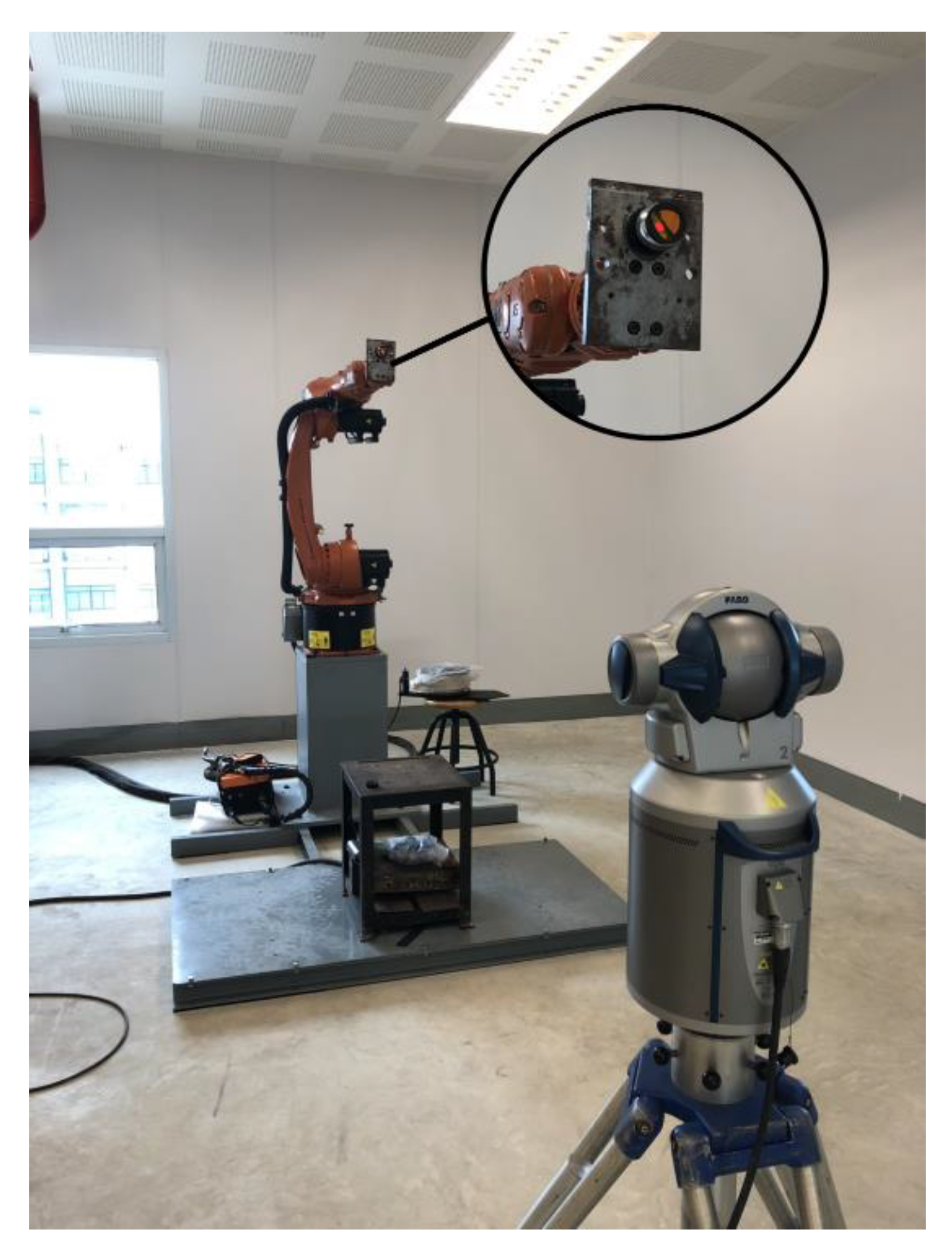
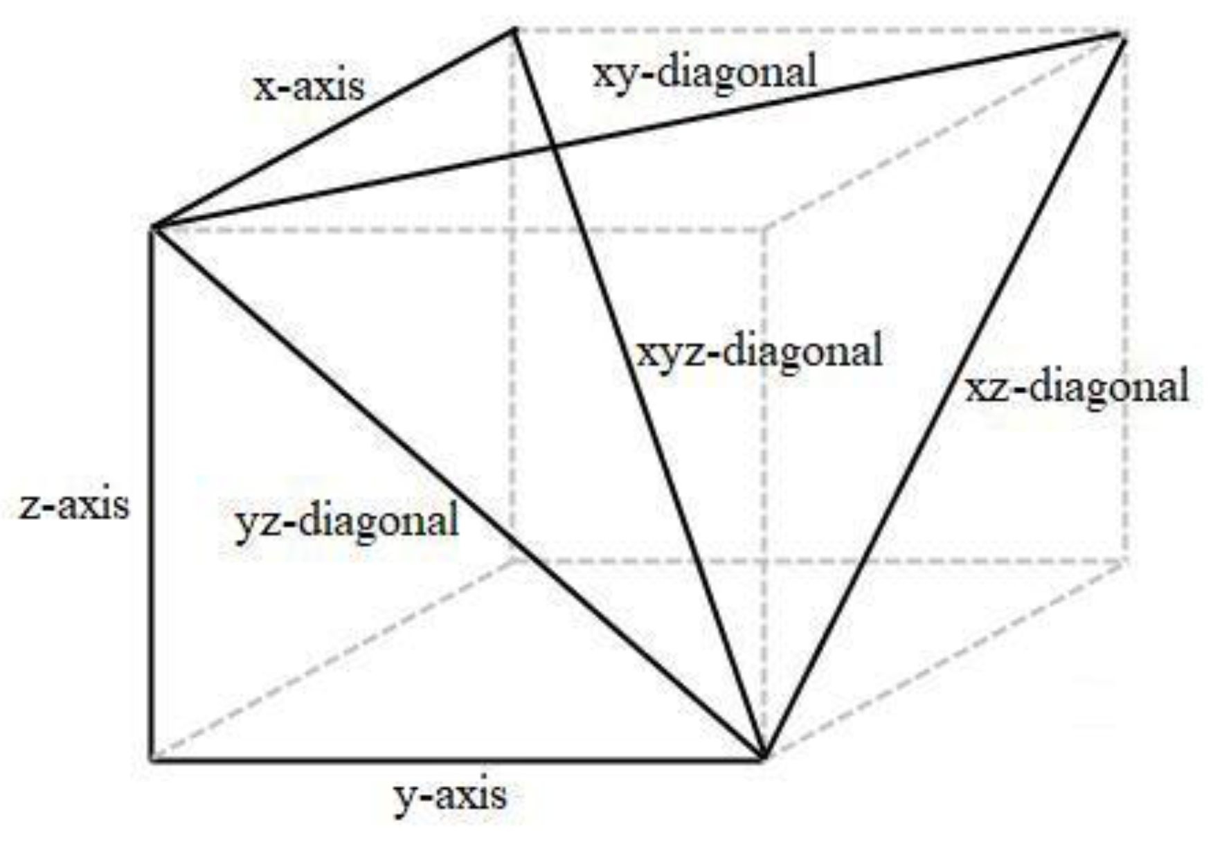
3.1. Experimental Setup

The installation which is shown in Figure 4 was used for measuring the geometric errors in each joint of a KUKA KR5 robot with a Faro laser tracker ION model in interferometer mode. According to the product specifications of this laser tracker, it has an angular accuracy around 10 μm + 2.5 μm/m, distance measurement accuracy in interferometer mode of 8μm + 0.4 μm/m and resolution 0.16 μm. The repeatability of the robot is ±0.04 mm. Unfortunately, no information shows the positional accuracy of this robot. The position measurement was performed with a spherically mounted reflector (SMR), diameter 1.5-in installed at each joint of the robot. A jig fixture at end-effector dimensions is 136 × 100 × 12 mm. It is made of SS400. All measurements ware performed at a temperature varying between 32 and 35 °C. The location of the base frame of a robot must be in alignment with respect to the system coordinate frame of measurement software (CAM2 SmartInspect) with the laser tracker. The location of the base frame of the laser tracker was constructed by the coordinate system in software with “plane-line-point” mode. A plane is the base frame which uses the table that places the robot as the plane of the coordinate system. A line is the direction of the base frame which uses the two screw positions that fasten the robot on base for a constructed line as the Y axis. A point is the origin point of the base frame which uses the center of the cylinder of A1 axis so that it can directly measure errors.

In the first test, in the axis-by-axis measurements, each joint was rotated separately. For each robot axis, a circle was fitted. From this circle, the robot axis was extracted. The position of SMR was measured when each joint was displaced by equal increment within an interval, as defined in

Table 2. A range of motion and pose for each joint for test.

Joint	Interval (°)	Increment (°)	Pose (°)
1	−54 to 126	9	−
2	−160 to −24	8	A1 −90
3	0 to 140	7	A1 90, A2 −90
4	−180 to 180	18	A1 0, A2 −90, A3 90
5	−108 to 108	12	A1 90, A2 −90, A3 90, A4 0
6	−180 to 180	18	A1 0, A2 −90, A3 90, A4 0, A5 0

. The errors were calculated with respect to the circle center at the joint axis.

The second test was to measure and compare the robot end-effector position between the normal kinematic model Equation (3) and the proposed kinematic model Equation (7), which was installed with a jig-fixture. This study was based on the 12-line method [14] to identify error parameters. The position errors were measured in seven directions of robot space as x-axis, y-axis, z-axis, xy-diagonal, yz-diagonal, xz-diagonal and xyz-diagonal, as shown in Figure 5. There are 11 poses in each direction. Therefore, there is a total of 77 poses in this experiment, and the volumetric error workspace is $x\times y\times z=600\times 800\times 400$ mm³. Both tests were repeated 30 times for each pose.

The third test was to verify geometric error compensation, which was compensated by offline programming. The measurement method was the same as in the second test. The modified forward kinematic model is defined as

$$T_{modified}=A_1{E}_1^{-1}{A}_2{E}_2^{-1}{A}_3{E}_3^{-1}{A}_4{E}_4^{-1}{A}_5{E}_5^{-1}{A}_6{E}_6^{-1}{A}_7$$

(11)

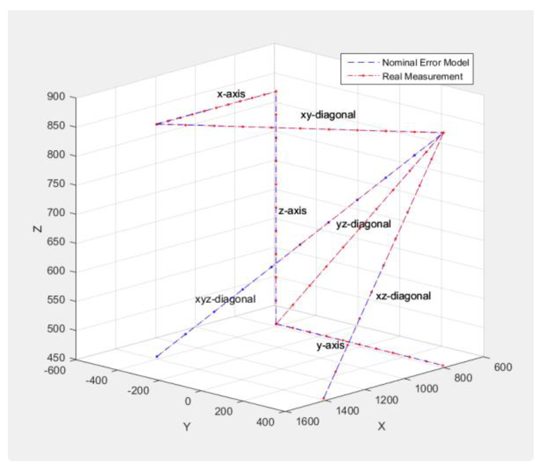
3.2. Experimental Data Analysis

This section presents the analysis measurement data from the first test. Figure 6 shows the data of the points captured in each joint in 3D space, which can be represented as a circle, as shown in Figure 7. The normal direction of the circle was fitted in the measuring software as A1 axis as the z-axis and A2 to A6 axis as the x-axis of the robot base frame. The circle fitting method can be separated into four steps:

• Using Singular Value Decomposition (SVD) to find the best fitting plane to the set of the mean centered point [26,27];

A plane can be found that fits as closely as possible to a set of 3D points, and the closeness is measured by software between the plane and the points. The normal vector $n$ for the fitting plane can be defined from SVD as

$$A=U\Sigma V^T$$

(12)

where $U,V$ are unitary matrices and $\Sigma$ is a diagonal matrix containing singular values ${\sigma }_1\ge {\sigma }_2\ge {\sigma }_3\ge 0$. The SVD can be written as

$$\begin{array}{ll}{\Vert An\Vert }^2& ={\Vert U\Sigma V^{T}n\Vert }^2={\Vert \Sigma V^{T}n\Vert }^2\\ & ={\left({\sigma }_1{b}_1\right)}^2+{\left({\sigma }_2{b}_2\right)}^2+{\left({\sigma }_3{b}_3\right)}^2\end{array}$$

(13)

where $b=V^{T}n$. Thus, the expression is obviously minimized by choosing $b={(0,0,1)}^T$ since ${\sigma }_3$ is the lowest singular value. Finally, $n$ is found by solving $V^{T}n=b$, which is trivial since $V$ is an unitary matrix, so $V{V}^T=I$.

$$V{V}^{T}n=Vb$$

(14)

$$n=Vb=V\left(\begin{array}{c}0\\ 0\\ 1\end{array}\right)=V\left(:,3\right)$$

(15)

The expression ${\Vert An\Vert }^2$ is minimized if, and only if, the normal vector $n$ is chosen as the 3rd column of matrix $V$;

2.

Using the Rodrigues rotation to project the mean center point onto the fitting plane in new 2D coordinates [28].

The Rodrigues rotation formula projects 3D points on the fitting plane, P, to new 2D X-Y coordinates in the coordinate system plane. The Rodrigues rotation formula can be written as

$$P_{rot}=P\cos \theta +\left(k\times P\right)\sin \theta +k\left(k\cdot P\right)\left(1-\cos \theta \right)$$

(16)

where the angle $\theta$ is measured from the original 3D normal vector to the new 2D normal vector and vector $k$ is axis of the rotation vector as a cross product between the 3D normal vector and the new 2D normal vector. Thus, $k=n\times {\left(0,0,1\right)}^T$;

3.

Using the method of the least mean squares, fit a circle in the new 2D coordinates and get the circle center. The circle’s equation in 2D for a circle with center ${\left(x_c,y_c\right)}^T$ can be written as

$$x^2+y^2+c_{1}x+c_{2}y+c_3=0$$

(17)

where the vector $c={\left(c_1,c_2,c_3\right)}^T$ for unknown parameters. Applied to all points, it yields to a system of liner equations $Ac=b$, where

$$b=\left(\begin{array}{c}{x}_0^2+y_0^2\\ ⋮\\ x_{n-1}^2+y_{n-1}^2\end{array}\right)$$

(18)

An approximate solution can be found by method of the least mean squares, which minimizes the square sum of residuals ${\Vert b-Ac\Vert }^2$, thus

$$c=\underset{c\in R^3}{\arg \min }{\Vert b-Ac\Vert }^2$$

(19)

4.

Transform the circle center back to 3D coordinates by the Rodrigues rotation, as in step (2), but the angle $\theta$ in this step is measured from the new 2D normal vector to the original 3D normal vector, and vector k is the axis of the rotation vector as a cross product between the 2D normal vector and the 3D normal vector. Thus, $k={\left(0,0,1\right)}^T\times n$.

From Figure 7, there are two circles, $C_1$ and $C_2$, that are composed of a circle center point ($c_n$ and $c_r$, as in Equation (17)) and normal vector (${\widehat{n}}_n$ and ${\widehat{n}}_r$, as in Equation (15)), respectively. The circle $C_1$ is the nominal or target circle, and $C_2$ is the approximate circle, fitted from measuring points. The $e_{\beta }$ and $e_{\gamma }$ are the angular error along the x and y axes between two normal vector ${\widehat{n}}_n$ and ${\widehat{n}}_r$. $e_x$, $e_y$ and $e_z$ are the position errors in the x, y and z axes between the circle center point ($c_n$ and $c_r$).

4. Results of the Experiment

4.1. Geometric Error Calculated

Two angular errors ($e_{\beta }$, $e_{\gamma }$) and three positional errors ($e_x$, $e_y$, $e_z$) of each joint ware measured by the laser tracker that was presented in Section 3. A summary of all 30 errors is demonstrated in

Table 3. Geometric error of each joint.

Joint	${\mathit{e}}_{\mathit{\beta }}$	${\mathit{e}}_{\mathit{\gamma }}$	${\mathit{e}}_{\mathit{x}}$	${\mathit{e}}_{\mathit{y}}$	${\mathit{e}}_{\mathit{z}}$
1	−0.0331	0.0218	−0.3702	−0.7174	−0.0005
2	0.1813	0.0068	−0.4168	0.3069	0.0014
3	−0.0069	0.0034	0.9521	0.5143	0.0001
4	−0.0295	0.0031	0.3414	−0.2313	0.0002
5	−0.0198	0.0361	0.4848	0.3526	0.0004
6	−0.0129	0.0772	−0.4767	−0.4767	0.0007

.

4.2. A Comparison of Kinematic Model Calculation and Real Measurement

A total of 30 geometric errors were calculated for the kinematic model with errors. An error kinematic model was calculated using the method in Section 2. Figure 8 shows a position error comparison between the kinematic model with the error calculation and real measurement from the laser tracker in the second test. The comparison results have the maximum difference of x-axis direction by ±0.56 mm, y-axis direction by ±0.58 mm, z-axis direction by ±0.52 mm, xy-diagonal direction by ±0.66 mm, xz-diagonal direction by ±0.84 mm, yz-diagonal direction by ±0.65 mm and xyz-diagonal direction by ±0.61 mm.

4.3. Tolerancing of Geometric Errors

This section shows the tolerancing of geometric errors following Section 2.3. The error angle of the normal axis, $\theta$ can be defined as

$$\theta =\sqrt{e_{\beta }^2+e_{\gamma }^2}$$

(20)

From Section 4.1, tolerancing from Equation (8) can be calculated for each joint of the robot, as in

Table 4. Tolerancing of each joint.

Joint	Perpendicularity or Parallelism	Position
	δ (mm)	x	y	z
1	0.0346	−0.3702	−0.7174	−0.0005
2	0.1742	−0.4168	0.3069	0.0014
3	0.0013	0.9521	0.5143	0.0001
4	0.0145	0.3414	−0.2313	0.0002
5	0.0086	0.4848	0.3526	0.0004
6	0.0164	−0.4767	−0.4767	0.0007

.

4.4. Kinematic Error Compensation

In order to verify the feasibility of the positional error model and error compensation method in this study, the geometric error that was calculated in Section 4.1 was compensated in Equation (11). The geometric error was compensated by offline programming. The results of the position errors were performed, compensated and uncompensated, as shown in Figure 9, Figure 10 and Figure 11. The results show the absolute positional errors that were calculated using the following equation

$$e=\sqrt{e_x^2+e_y^2+e_z^2}$$

(21)

where e_x, e_y and e_z are the position errors on the x, y and z axis, respectively. According to the experiment results, the positional error was maximally reduced on each direction as follows: x-axis direction by 90%, y-axis direction by 88%, z-axis direction by 81%, xy-diagonal direction by 80%, xz-diagonal direction by 71%, yz-diagonal direction by 74% and xyz-diagonal direction by 85%.

5. Conclusions

In this study, an analysis of a joint geometric error affecting a robot end-effector was presented. Geometric Dimensioning and Tolerancing (GD&T) was applied to explain the geometric errors. The transformation kinematic and geometric errors were developed by the combination of translation methods.

This method was used in the error analysis of a six-axis robot. The tolerances of each joint and the error compensation method were proposed and verified with experiments. The first experiment found a total of geometric errors and tolerancing of geometric errors. The second experiment results showed a position error comparison between the kinematic model with error calculation and real measurement from the laser tracker. The comparison position errors revealed that the maximum difference of all directions was ±0.84 mm. Likewise, the third experiment results showed before and after compensation errors. All direction compensations were found with a maximum positional error of ±3.98 mm. However, a compensation error method in this study reduced the maximum position error by 90%. Therefore, the proposed method can effectively improve the joint geometric error and compensated error in a six-axis robot.

References

1. Gong, C.; Yuan, J.; Ni, J. Nongeometric error identification and compensation for robotic system by inverse calibration. Int. J. Mach. Tools Manuf. 2000, 40, 2119–2137. [Google Scholar] [CrossRef]
2. Meggiolaro, M.A.; Dubowsky, A.; Mavroidis, C. Geometric and elastic error calibration of a high accuracy patient positioning system. Mech. Mach. Theory 2005, 40, 415–427. [Google Scholar] [CrossRef]
3. Jang, J.H.; Kim, S.H.; Kwak, Y.K. Calibration of geometric and non-geometric errors of an industrial Robot. Robotica 2001, 19, 311–321. [Google Scholar] [CrossRef] [Green Version]
4. Weidong, Z.; Guanhua, L.; Huiyue, D.; Yinglin, K. Positioning error compensation on two-dimensional manifold for robotic machining. Robot. Comput. Integr. Manuf. 2019, 59, 394–405. [Google Scholar]
5. Mohnke, C.; Reinkober, S.; Uhlmann, E. Constructive methods to reduce thermal influences on the accuracy of industrial robots. Procedia Manuf. 2019, 33, 19–26. [Google Scholar] [CrossRef]
6. Li, R.; Zhao, Y. Dynamic error compensation for industrial robot based on thermal effect model. Measurement 2016, 88, 113–120. [Google Scholar] [CrossRef]
7. Barakat, N.A.; Elestawi, M.A.; Spence, A.D. Kinematic and geometric error compensation of a coordinate measuring machine. Int. J. Mach. Tools Manuf. 2000, 40, 833–850. [Google Scholar] [CrossRef]
8. Ramesh, R.; Mannan, M.A.; Poo, A.N. Error compensation in machine tools—A review: Part I: Geometric, cutting-force induced and fixture-dependent errors. Int. J. Mach. Tools Manuf. 2000, 9, 1235–1256. [Google Scholar] [CrossRef]
9. Okafor, A.C.; Ertekin, Y.M. Derivation of machine tool error models and error compensation procedure for three axes vertical machining center using rigid body kinematics. Int. J. Mach. Tools Manuf. 2000, 8, 1199–1213. [Google Scholar] [CrossRef]
10. Chanal, H.; Duc, E.; Ray, P.; Hascoet, J.Y. A new approach for the geometrical calibration of parallel kinematics machines tools based on the machining of a dedicated part. Int. J. Mach. Tools Manuf. 2007, 47, 1151–1163. [Google Scholar] [CrossRef]
11. Cetinkunt, S.; Tsai, R.L. Position error compensation of robotic contour end-milling. Int. J. Mach. Tools Manuf. 1990, 30, 613–627. [Google Scholar] [CrossRef]
12. OH, Y. Study of Orientation Error on Robot End Effector and Volumetric Error of Articulated Robot. Appl. Sci. 2019, 9, 5149. [Google Scholar] [CrossRef] [Green Version]
13. Chen, J.X.; Lin, S.W.; Zhou, X.L. A comprehensive error analysis method for the geometric error of multi-axis machine tool. Int. J. Mach. Tools Manuf. 2016, 106, 56–66. [Google Scholar] [CrossRef]
14. Chen, J.; Chao, L.M. Positioning error analysis for robot manipulators with all rotary joints. IEEE J. Robot. Autom. 1987, 3, 539–545. [Google Scholar] [CrossRef]
15. Zeng, Y.; Tian, W.; Liao, W. Positional error similarity analysis for error compensation of industrial robots. Robot. Comput. Integr. Manuf. 2016, 42, 113–120. [Google Scholar] [CrossRef]
16. Zhu, S.; Ding, G.; Qin, S.; Lei, J.; Zhuang, L.; Yan, K. Integrated geometric error modeling, identification and compensation of CNC machine tools. Int. J. Mach. Tools Manuf. 2012, 52, 24–29. [Google Scholar] [CrossRef]
17. Nguyen, H.N.; Zhou, J.; Kang, H.J. A new full pose measurement method for robot calibration. Sensors 2013, 13, 9132–9147. [Google Scholar] [CrossRef] [Green Version]
18. Mavroidis, C.; Dubowsky, S.; Drouet, P.; Hintersteiner, J.; Flanz, J. A systemtic error analysis of robotic manipulator: Application to a high performance medical robot. In Proceedings of the International Conference on Robotics and Automation, Albuquerque, NM, USA, 20–25 April 1997; pp. 980–985. [Google Scholar]
19. Raksiri, C.; Parnicjkun, M. Geometric and force errors compensation in 3-axis CNC milling machine. Int. J. Mach. Tools Manuf. 2004, 44, 1283–1291. [Google Scholar] [CrossRef]
20. Wan, A.; Song, L.; Xu, J.; Liu, S.; Chen, K. Calibration and compensation of machine tool volumetric error using a laser tracker. Int. J. Mach. Tools Manuf. 2018, 124, 126–133. [Google Scholar] [CrossRef]
21. Cao, C.T.; Do, V.P.; Lee, B.R. A Novel Indirect Calibration Approach for Robot Positioning Error Compensation Based on Neural Network and Hand-Eye Vision. Appl. Sci. 2019, 9, 1940. [Google Scholar] [CrossRef] [Green Version]
22. Nubiola, A.; Bonev, I.A. Absolute calibration of an ABB IRB 1600 robot using a laser tracker. Robot. Comput. Integr. Manuf. 2013, 29, 236–245. [Google Scholar] [CrossRef]
23. Li, C.; Liu, X.; Li, R.; Song, H. Geometric Error Identification and Analysis of Rotary Axes on Five-Axis Machine Tool Based on Precision Balls. Appl. Sci. 2020, 10, 100. [Google Scholar] [CrossRef] [Green Version]
24. Santolaris, J.; Gines, M. Uncertainty estimation in robot kinematic calibration. Robot. Comput. Integr. Manuf. 2013, 29, 370–384. [Google Scholar] [CrossRef]
25. Niku, S.B. Introduction to Robotics Analysis, Systems, Applications; Prentice Hall: New Jersey, NJ, USA, 2001. [Google Scholar]
26. Pechard, P.Y.; Tournier, C.; Lartigue, C.; Lugarin, J.P. Geometrical deviations versus smoothness in 5-axis high-speed flank millings. Int. J. Mach. Tools Manuf. 2009, 49, 454–461. [Google Scholar] [CrossRef] [Green Version]
27. Hayat, A.A.; Body, R.A.; Saha, S.K. A geometric approach for kinematic identification of an industrial robot using a monocular camera. Robot. Comput. Integr. Manuf. 2019, 57, 329–346. [Google Scholar] [CrossRef]
28. Enferad, J.; Shahi, A. On the position analysis of a new spherical parallel robot with orientation applications. Robot. Comput. Integr. Manuf. 2016, 37, 151–161. [Google Scholar] [CrossRef]
Figure 1. Schematic diagram of KUKA robot as: (a) KUKA KR5 schematic model; (b) KUKA KR5 nominal dimension.
Robotics 09 00027 g001
Figure 2. Frame displacement due to errors.
Robotics 09 00027 g002
Figure 3. Tolerancing Analysis. (a) Tolerancing as define in detail drawing; (b) Tolerancing direction.
Robotics 09 00027 g003
Figure 4. Experiment setup.
Robotics 09 00027 g004
Figure 5. The seven directions measurement.
Robotics 09 00027 g005
Figure 6. Data set of the points captured in each joint.
Robotics 09 00027 g006
Figure 7. A represented circle, C 1 and C 2 , of the nominal and measuring circle.
Robotics 09 00027 g007
Figure 8. Nominal model error and real measurement comparison.
Robotics 09 00027 g008
Figure 9. Position error of major direction.
Robotics 09 00027 g009
Figure 10. Position error of 2d diagonal direction.
Robotics 09 00027 g010
Figure 11. Position error of 3d diagonal direction.
Robotics 09 00027 g011