Article

MallARD: An Autonomous Aquatic Surface Vehicle for Inspection and Monitoring of Wet Nuclear Storage Facilities

School of Electrical and Electronic Engineering, The University of Manchester, Oxford Road, Manchester M13 9PL, UK
*
Author to whom correspondence should be addressed.
Robotics 2019, 8(2), 47; https://doi.org/10.3390/robotics8020047
Submission received: 31 March 2019 / Revised: 21 May 2019 / Accepted: 14 June 2019 / Published: 18 June 2019
(This article belongs to the Special Issue Robotics in Extreme Environments)

Abstract

:
Inspection and monitoring of wet nuclear storage facilities such as spent fuel pools or wet silos is performed for a variety of reasons, including nuclear security and characterisation of storage facilities prior to decommissioning. Until now such tasks have been performed by personnel or, if the risk to health is too high, avoided. Tasks are often repetitive, time-consuming and potentially dangerous, making them suited to being performed by an autonomous robot. Previous autonomous surface vehicles (ASVs) have been designed for operation in natural outdoor environments and lack the localisation and tracking accuracy necessary for operation in a wet nuclear storage facility. In this paper the environmental and operational conditions are analysed, applicable localisation technologies selected and a unique aquatic autonomous surface vehicle (ASV) is designed and constructed. The ASV developed is holonomic, uses a LiDAR for localisation and features a robust trajectory tracking controller. In a series of experiments the mean error between the present ASV’s planned path and the actual path is approximately 1 cm, which is two orders of magnitude lower than previous ASVs. As well as lab testing, the ASV has been used in two deployments, one of which was in an active spent fuel pool.

Graphical Abstract

1. Introduction

The motivation for the present research is to facilitate the automation of inspection and monitoring tasks in nuclear fuel storage pools and wet silos by the provision of a suitable aquatic autonomous surface vehicle (ASV). Radioactive material such as spent fuel and legacy waste is typically stored underwater in deep pools, where the water provides both radiation shielding and cooling. Radioactive material usually remains in spent fuel pools (SFPs) for 10 or more years before being reprocessed or sent for long term storage [1]. SFPs are routinely monitored and inspected by the facility operators and external organisations. Inspection and monitoring is performed for a range of purposes, including radiation monitoring, assessment of the condition of the spent fuel rods and nuclear security.
Presently, inspection and monitoring of SFPs is reliant on personnel to deploy the required sensors and equipment, usually from a movable bridge above the pool; tasks are often repetitive and time consuming and therefore suited to automation [2]. Moreover, due to the proximity to radioactive material, access is restricted, working can be awkward and physically demanding due to the need to wear protective clothing and there is a potential health risk to the operator.

1.1. Environment

Spent fuel storage pools (Figure 1) are usually over 10 m deep with high walls and are between 5 m and 50 m in length, although larger pools are typically segmented into smaller walled areas. SFPs are generally indoor, well-lit and constructed from poured concrete. The walls and surroundings can be plain and featureless, or feature-rich with piping, fixtures and other equipment; the same is true of the ceiling above. Looking down towards the fuel from the water surface, the water is deep but usually clear in modern SFPs meaning that feature-rich video of the stored fuel may be available. However, in legacy SFPs and wet silos clarity of the water cannot be relied upon and lighting could be variable or non-existent. For both SFPs and wet silos the environment may be considered time invariant, operations that involve change to the environment such as fuel handling can be scheduled around inspection and monitoring tasks. Water temperature in an SFP is usually around 40 °C [3] and water circulation systems may create strong currents in certain areas of the pool. The magnetic field in and surrounding the SFP or wet silo is likely to contain interference from equipment in the vicinity or ferrous content of the concrete walls [4].

1.2. Application

To formulate the ASVs operational requirements, two specific application examples are discussed in the following sections.

1.2.1. Deployment of an Improved Cerenkov Viewing Device

An improved Cerenkov viewing device (ICVD) is a light intensifying device that is optimised for viewing Cherenkov glow emitted from fuel rods an SFP. This is the instrument most commonly used by IAEA inspectors to confirm the presence of spent fuel in SFPs [2]. Spent fuel assemblies are characterised by their Cherenkov glow pattern. The Cherenkov glow is very bright in the region directly above the fuel rods. Therefore, to distinguish an irradiated fuel assembly from a non-fuel item the ICVD must be carefully aligned above the fuel rod. Fuel rods are typically around 1 cm in diameter [5] so it is reasonable to assume that the vehicle should be capable of control accuracy of a similar magnitude. Control accuracy is also important to prevent collisions when the vehicle is navigating close to walls and obstacles. For the ICVD to produce clear unblurred video from which individual fuel rods can be verified, the vehicle must move slowly over the fuel assemblies with minimal variation in pitch and roll. Assuming that a minimum of 2 s of video would be required while the vehicle passes over a typical 20 cm wide fuel assembly [5], a reasonable maximum scanning speed is 0.1 m/s. Maintaining velocities and accelerations at low levels will also help minimise pitch and roll of the ASV caused by misalignment of the centres of thrust, drag and mass; although it is possible to mechanically stabilise the ICVD by mounting it on an active gimbal, as discussed in Section 3.1. For efficient coverage, the ASV should be capable of following straight lines above rows of fuel rods. To maintain ICVD orientation whilst scanning, a holonomic ASV is preferred.

1.2.2. Radiation Monitoring of Pool Walls

The ASV may be used to deploy radiation detectors to monitor the activity of the walls of the pool or silo. This is particularly necessary when legacy pools or silos are drained for decommissioning and decontamination of the pool walls must be verified. Radiation detectors are often highly sensitive to the distance from the object they are measuring and usually must be held still for a period of time while the measurement is performed. Therefore, the ASV will need to be able to hold a pose with good accuracy, preferably sub-centimetre. If measurements are to be repeated following decontamination, it is important that the ASV can return to a previously held position to repeat the detection task. Stability of the payload is less important in this case because the distance between the sensor and the object is much smaller.

1.2.3. General Requirements

The ASV will be required to operate on the surface of the water and have a large flexible payload area that can carry a wide range of sensing equipment. To reduce the risk of contamination and simplify setup and operation, the system should be standalone and not require the use of any beacons or goalposts. Setup complexity and operator time should be minimised and the ASV should be easy to clean and eliminate any trace of contaminated water so that the system can be safely transported and redeployed.

1.3. Review of Existing ASVs

To date, a range of ASVs have been developed [6,7,8,9,10], however, most are large vehicles that have been designed for operation in marine environments and lakes [7,8,11]. They rely on unsuitable sensor packages and lack the control accuracy required for operation in SFPs or wet silos. In the literature, the best performing ASVs in terms of path tracking abilities achieve an average path tracking error of around 1 m [7,8]. In [7] Dunbabin and Grinham evaluate the tracking accuracy of an autonomous surface vehicle in Lake Wivenhoe, Australia. The vehicle is a catamaran which is several metres in length, utilises GPS for navigation and has a tracking accuracy of approximately 1 m. While fit for purpose, this vehicle is clearly not suited for deployment in an SFP or wet silo because the GPS will not work indoors and the vehicle does not provide the required tracking accuracy.
As there are currently no ASVs that are suited to the unique environment of a wet nuclear storage facility, the present paper gives detail of a novel ASV that is appropriately sized, has a localisation system that works in confined GPS denied environments without the use of external infrastructure and has cm accurate path tracking ability.

1.4. Contributions

  • An analysis of a range of localisation technologies that are applicable to an autonomous aquatic surface vehicle operating in a confined environment.
  • Detail of the mechanical and software design of a uniquely capable autonomous aquatic surface vehicle.
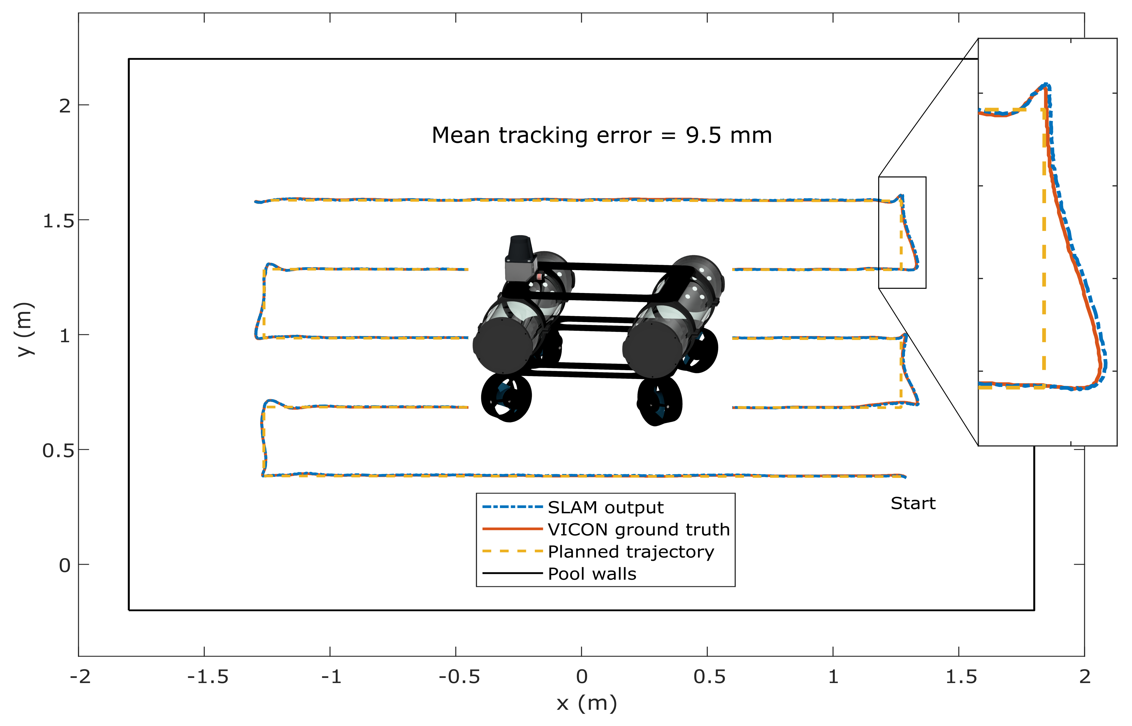
  • Experimental work proving that the ASV is capable of meeting the requirements of two example applications: Straight path tracking and position holding.

2. Localisation Technologies

In Section 2.1 the viability of commercially available technologies that can provide or aid localisation are discussed. In Section 2.2 the findings are summarised and the localisation technologies used in the present work are selected.

2.1. Analysis of Relevant Localisation Technologies

Global navigation satellite systems (GNSS) are common place on marine vehicles but must be ruled out in the present case due to the fact that most facilities will be indoors. Even if GNSS was available, the nominal accuracy of a good quality GNSS is around 1 m, degrading at approximately 0.22 m for each 100 km from the broadcast site [12].
Computer vision (including the use of monocular, stereo and RGBD cameras) can be used to provide odometry [13] as well as simultaneous location and mapping (SLAM) [14] both above and below the waterline. However, visual systems fail to function reliably in environments with too few or too many salient features, where lighting is poor or changeable and during rapid movements of the camera [15]. As stated in Section 1.1, for the present problem scenes are often feature-sparse, water may be turbid and good lighting cannot be guaranteed; therefore a vision system cannot be employed without a reliable fall back system in place. For example, the AR drone [16] chooses between two visual SLAM algorithms dependent on conditions and has a fall back if neither algorithm can produce reliable localisation.
A LiDAR paired with an appropriate SLAM algorithm can provide highly accurate localisation above the water surface and has fast refresh rates [17]. LiDARs use light emitted by the sensor and the results do not deviate greatly in variable light conditions. The largely 2D environment in which the ASV operates and the presence of high surrounding walls makes use of 2D LiDAR a favourable choice. LiDAR technology is mature and a range of high accuracy, waterproof units in suitably sized packages are readily available. To compliment the 2D LiDAR, a variety of well tested 2D SLAM algorithms are also available to give pose information from the laser scan. Underwater LiDARs have recently become commercially available but are large, expensive and have safety constraints [18].
Inertial measurement units (IMUs) have very high refresh rates and can be used to improve the data obtained from an absolute measurement, such as LiDAR or GPS. By fusing the IMU with an absolute localisation method, the measurement accuracy of acceleration, velocity and displacement may be improved [17,19,20,21]. The IMU may also be used to fill gaps between the measurements of an absolute sensor, which is useful for fast acting control systems [22] and to rebuild a 2D or 3D scan [23]. 9-axis IMUs are composed of a 3-axis accelerometer, 3-axis gyro and 3-axis compass. As discussed in Section 1.1, magnetic disturbance is to be expected from the environment and the onboard electric motors, meaning that compass readings are likely to be noisy and unreliable; although, the compass is not necessary if another system, such as LiDAR localisation, is able to provide the ASV’s yaw angle. Accelerometers and gyroscopes are unaffected by the operational environment and with recent improvements in MEMS devices, reasonably priced, high accuracy, low power devices are now available.
Underwater acoustic systems (active sonars) paired with an appropriate SLAM algorithm can be used for absolute localisation [23,24,25,26,27]. Most systems are designed for and used in marine environments and their performance in confined highly structured environments is unquantified. Acoustic systems can suffer from multi-path issues or multiple echoes [18] and this will be amplified in confined environments. In comparison to a LiDAR, beam widths are wide and refresh rates are low, generally between 1–10 Hz [18,23,27,28]. A key benefit of acoustic systems is that they are unaffected by water turbidity [18,23]. Sonar localisation using beacons at known locations must be ruled out in the present case due to the requirements for minimal infrastructure and fast deployment. So called, sonar SLAM, using a mechanically scanned imaging sonar (MSIS) [4,26] would be possible, and given the typically slow movement required in the current context sonar SLAM may be a viable option, although difficult to make the case for if above surface LiDAR SLAM is available.

2.2. Technology Selection

The analysis presented in Section 2.1 is summarised in Table 1 and has clear findings. Due to high refresh rates and accuracy combined with low sensitivity to external conditions, the ASV developed in the present work uses a waterproof 2D LiDAR to provide absolute localisation. Addition of an IMU to improve relative state estimation was also shown to be viable but not necessary and investigation into the improvements that may be obtained from this addition will be the subject of future research. While not viable without a robust localisation system already in place as fail over, it may be possible to improve localisation by incorporation of vision systems for odometry or absolute localisation. Due to the significant increase in system complexity that would be required for an unquantified improvement, a vision system will not be incorporated at the present time. Since we have access to data from an above surface LiDAR, sonar SLAM will not be used.

3. Hardware Design

Figure 2 shows images derived from design files and a photo of the ASV named MallARD (sMall Autonomous Robotic Duck). The MallARD platform has six main parts: (I) Chassis plates, (II) pontoons, (III) electronics tray, (IV) battery tray, (V) four thrusters and (VI) waterproof 2D LiDAR. Section 3.1 and Section 3.2 give detail of the mechanical, propulsion and electronic design of the MallARD.

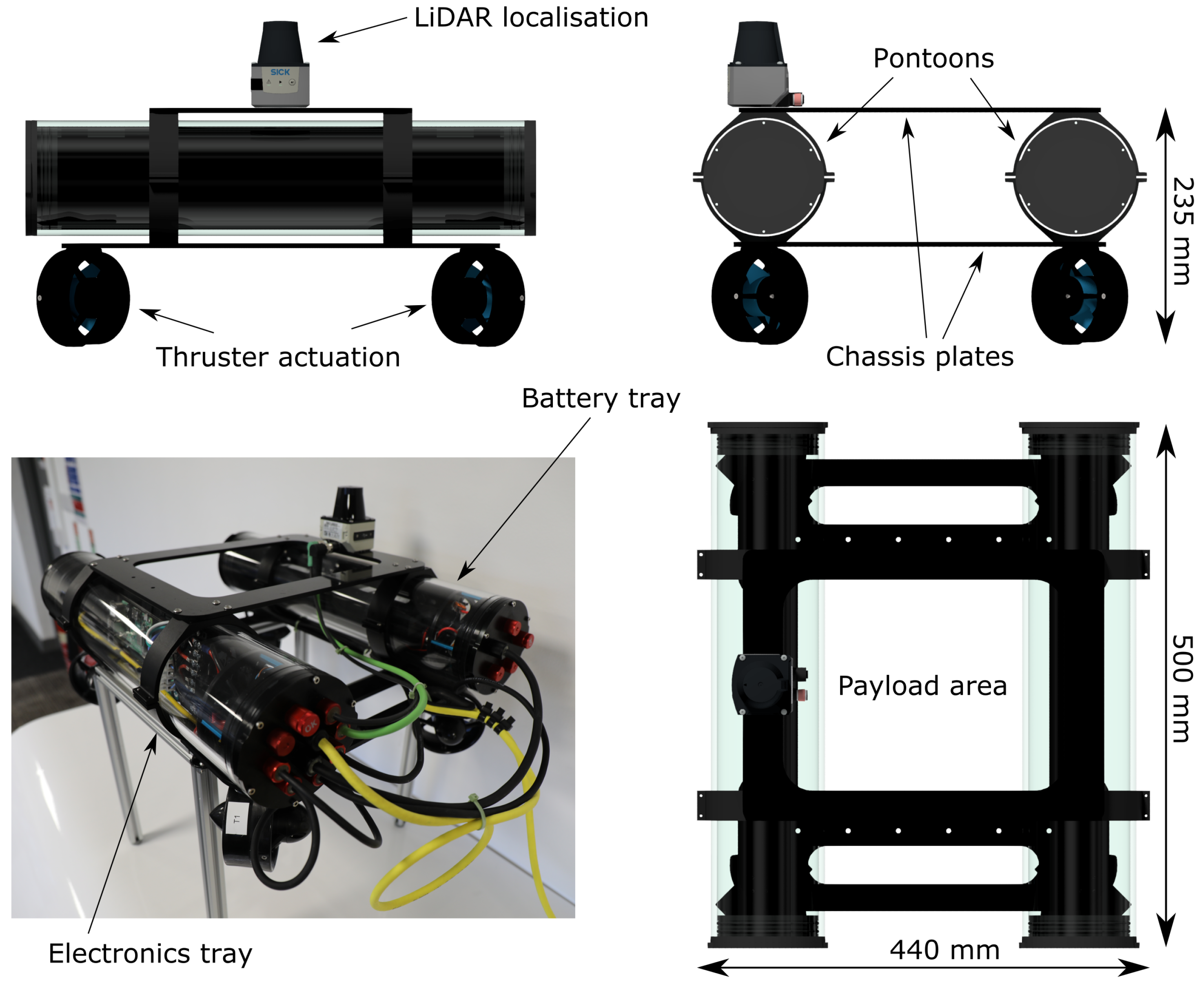
3.1. Mechanical and Propulsion
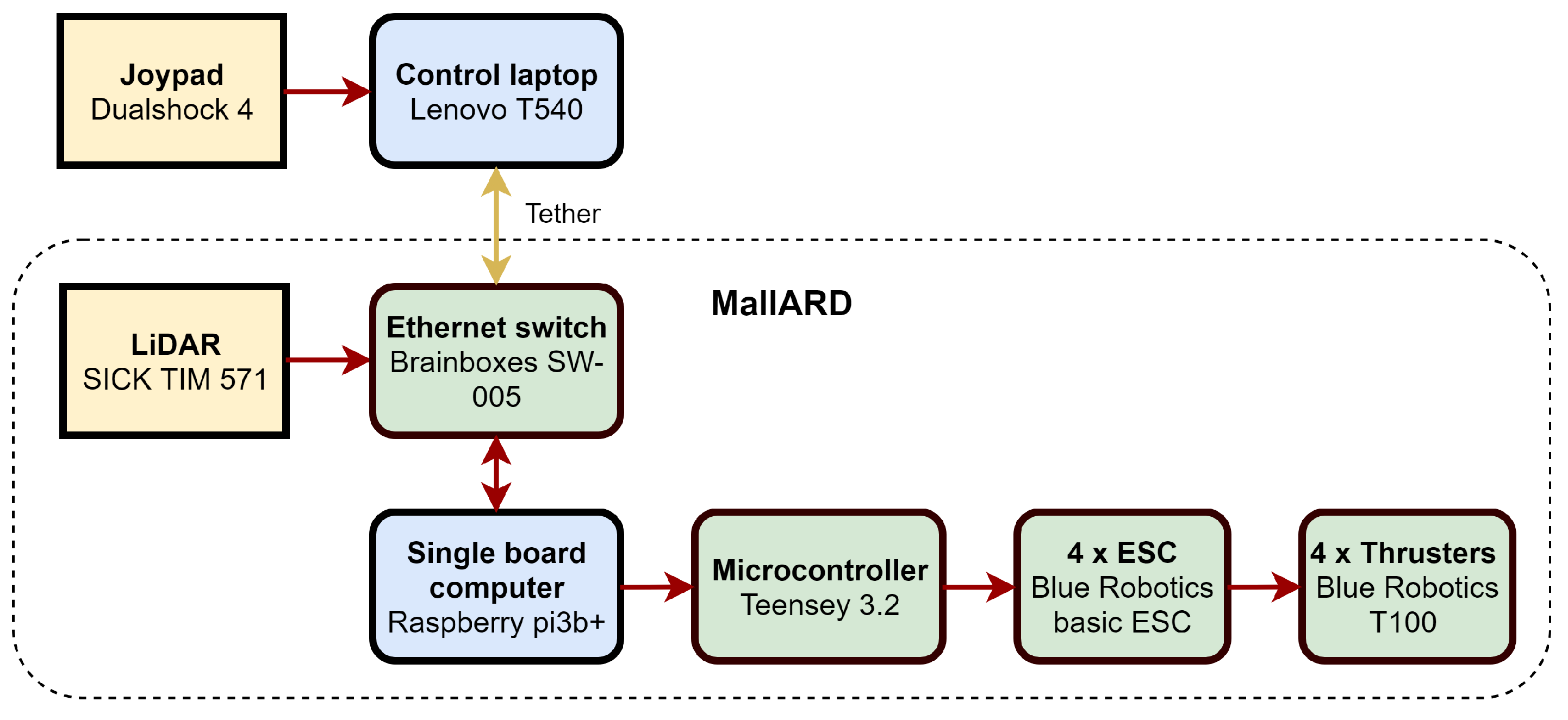
Previous ASVs have been underactuated [6,7,8,9,10] typically with catamaran design to maximise stability and minimise hydrodynamic drag in the surge direction. Due to the low speeds required, hydrodynamic drag magnitude will be small and since the robot must be holonomic (actuated in surge, sway and yaw) a classic catamaran design would have high drag bias in the sway direction compared to surge. The MallARD design is based on a stable platform that can move; the dual pontoon arrangement with wide spacing between the pontoons is simple, offers good stability and makes space through the centre of the robot for sensor payloads.
To provide locomotion, the robot has four bidirectional thrusters located at each of the four corners of the robot and angled at 45 degrees to the x or y axes. This thruster layout was selected due to its inherent symmetry in terms of drag and thrust and because the thrusters can be positioned such that they do not interfere with the central payload space. Geometric symmetry about the x z and y z planes means that drag forces will act through the central z-axis and not induce rotation. Thrust symmetry is important due to the thruster’s hydrodynamic design, for the same input magnitude, forward thrust is greater than backward. The chosen thruster layout accounts for this difference because motion in either the x b or y b direction requires an even balance of thrusters acting forward and backward, the same is true of yaw.
Pitch and roll actuation was not implemented on MallARD because it was found to be unnecessary for operation in small indoor pools. In indoor pools with normal levels of water circulation, the water surface is almost still. The combination of still water, a wide dual pontoon design and low operating speeds means that variations in pitch roll are small and have a negligible effect on the LiDAR operation. Active stabilisation would be necessary if higher stability is required for the payload or if the vehicle is operated in larger pools where the LiDAR scans risk missing the walls due to pitch and roll variation. In this case, adding an active stabilised platform (two-axis gimbal) to the ASV is a simpler solution than actuating the whole robot.
The MallARD is constructed from off-the-shelf components where possible, pontoons, thrusters, glanding system and circular clamps are from the Blue Robotics range. The chassis plates are laser cut from 5 mm Acetal sheet. The robot without payload weighs 10.5 kg.

3.2. Electronic

The MallARD is powered by two 5 Ah 11.1 V Lithium polymer batteries connected in series and housed in the front pontoon. All computational components are housed in the rear pontoon and the LiDAR is positioned on top of the front pontoon.
Figure 3 shows how the MallARD system components are electronically connected. At the core of the system is a single board computer running Linux and ROS (robot operating system). The single board computer receives information from the LiDAR and communicates with the control laptop via the onboard Ethernet switch. All autonomous functionality is performed onboard and the control laptop is only used for visualisation and manual control. When not in autonomous mode, the MallARD can be controlled using a joy-pad which sends data to the single board computer via the control laptop and Ethernet switch. Motion commands are sent from the single board computer over a serial connection to a micro-controller which generates a PWM signal that is sent to the electronic speed controllers (ESCs). The four ESCs receive power from the battery and provide a phased output on three cores to the brushless motors in the four thrusters.

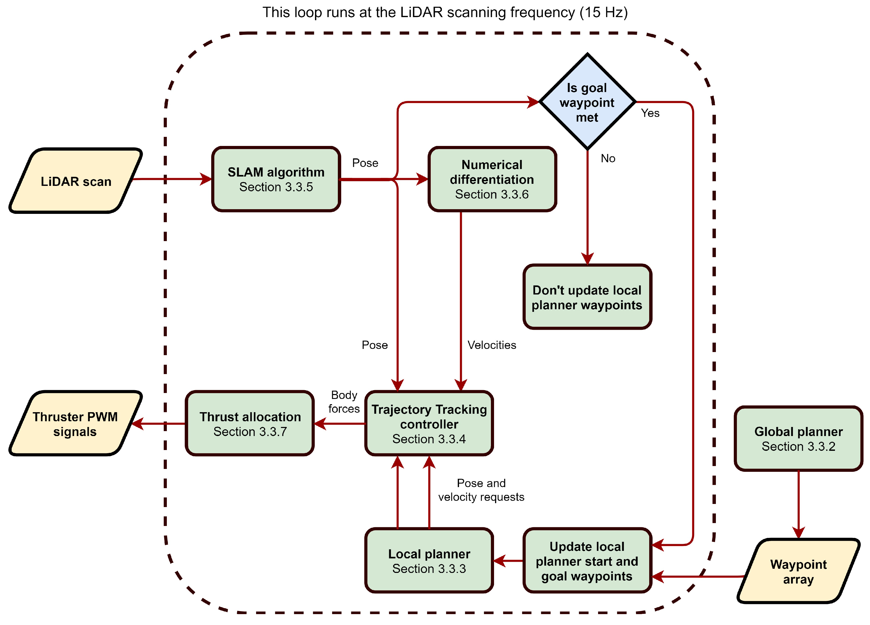
3.3. Localisation and Navigation System

Figure 4 presents MallARD’s localisation and autonomous navigation system. Inputs to the system are the LiDAR scan and the array of waypoints that is generated by the global planner. After the waypoint array is generated, the main loop runs each time a new LiDAR scan is produced. Throughout the present work the LiDAR scans at 15 Hz, making this the loop rate. At the centre of the main loop is the trajectory tracking controller and local planner. The local planner takes three variable inputs, start pose, goal pose and start time; these inputs are updated when a goal is met or if a goal has not been arrived at within a margin of the expected arrival time. When an update is made a new start time is recorded, the goal pose becomes the start pose and a new goal pose is taken from the next row of the waypoint array. Using the three variable inputs, the local planner determines the desired state vector s d t at any given time. The trajectory tracking controller receives s d t from the local planner and the actual state vector s t , which is generated using the LiDAR scan via a SLAM algorithm (Hector mapping [29]) and numerical differentiation block. The error between s d t and s t drives three proportional controllers that output the three-component force/moment vector τ n . In the thrust allocation block, the τ n vector is converted into the body frame using Equation (2), resulting in τ b . The three-component body frame force/moment vector τ b is converted into the four-component thruster frame force vector τ t using the thrust allocation matrix, detailed in Section 3.3.7. Individual thruster frame forces are then scaled to PWM values which are used to drive the ESCs and ultimately the thrusters.
To speed up development and reduce the need for pool access, all localisation and navigation software was initially built on the El-MallARD platform [30]: A holonomic ground robot that can mimic the physics of an aquatic surface vehicle. Details of the key functional components of the localisation and autonomous navigation system are presented in Section 3.3.1, Section 3.3.2, Section 3.3.3, Section 3.3.4, Section 3.3.5, Section 3.3.6 and Section 3.3.7.

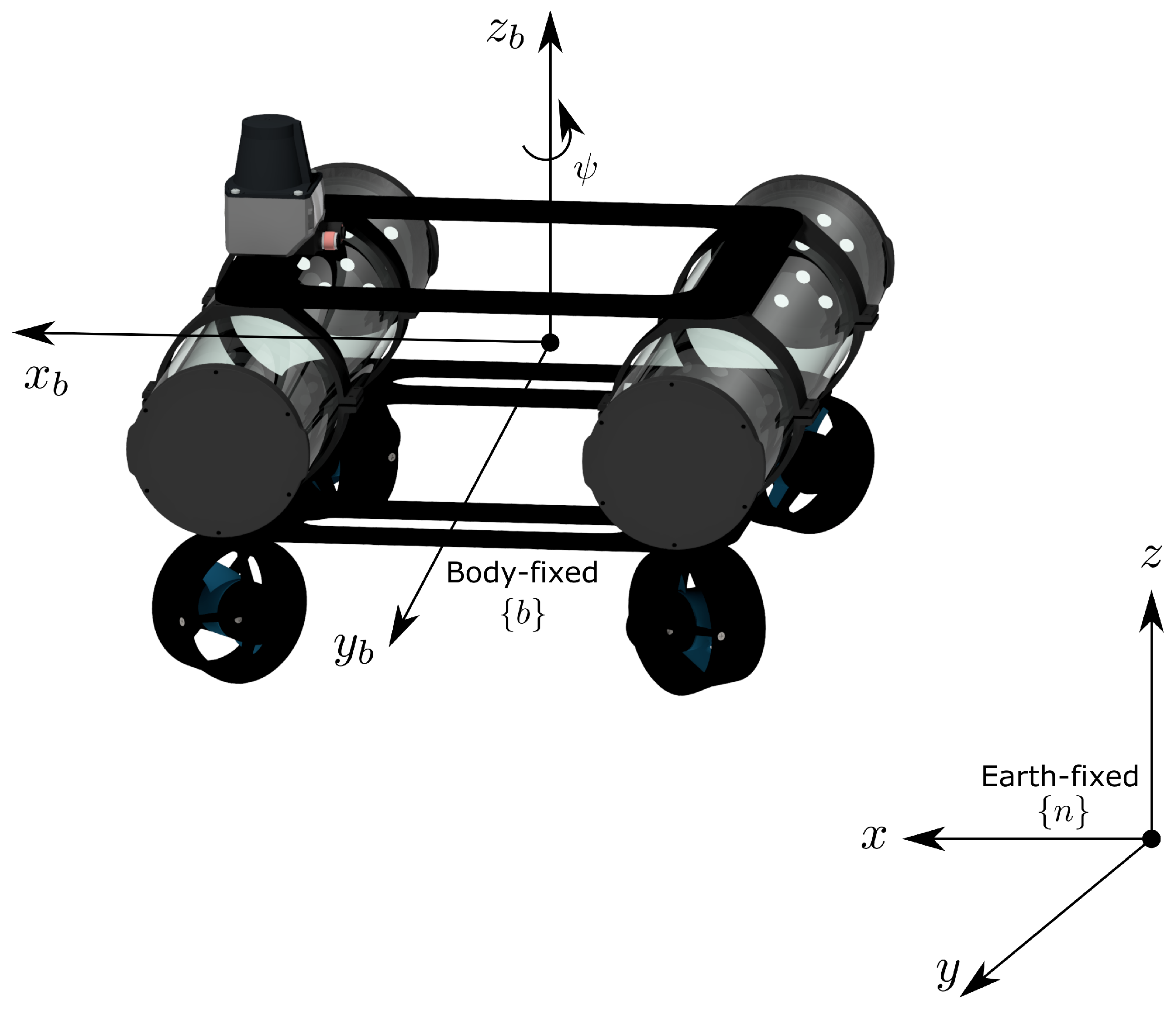
3.3.1. Coordinate System and Conventions

When analysing the 3 DOF motion of MallARD, it is convenient to use two coordinate frames as presented in Figure 5. All coordinate systems are right handed with the z-axis pointing upwards [31]. Using the notation convention of [32], the pose of the centre of the vessel in the earth-fixed navigation frame n is η = x , y , ψ T where x and y are Cartesian positions and ψ is the yaw angle about the z axis. The full state vector in the n frame is defined as s = η η ˙ = x , y , ψ , x ˙ , y ˙ , ψ ˙ T , where ˙ refers to differentiation with respect to time. In the present work, localisation and control is performed in the navigation reference frame n , although the MallARD’s propulsion output must ultimately be expressed in the body-fixed frame b . τ b and τ n are the vectors of propulsion forces and moments in b and n respectively. The rotation matrix R n b relates the navigation frame forces vector to the body frame force vector according to
τ b = R n b τ n
where
R n b ψ = cos ψ sin ψ 0 sin ψ cos ψ 0 0 0 1

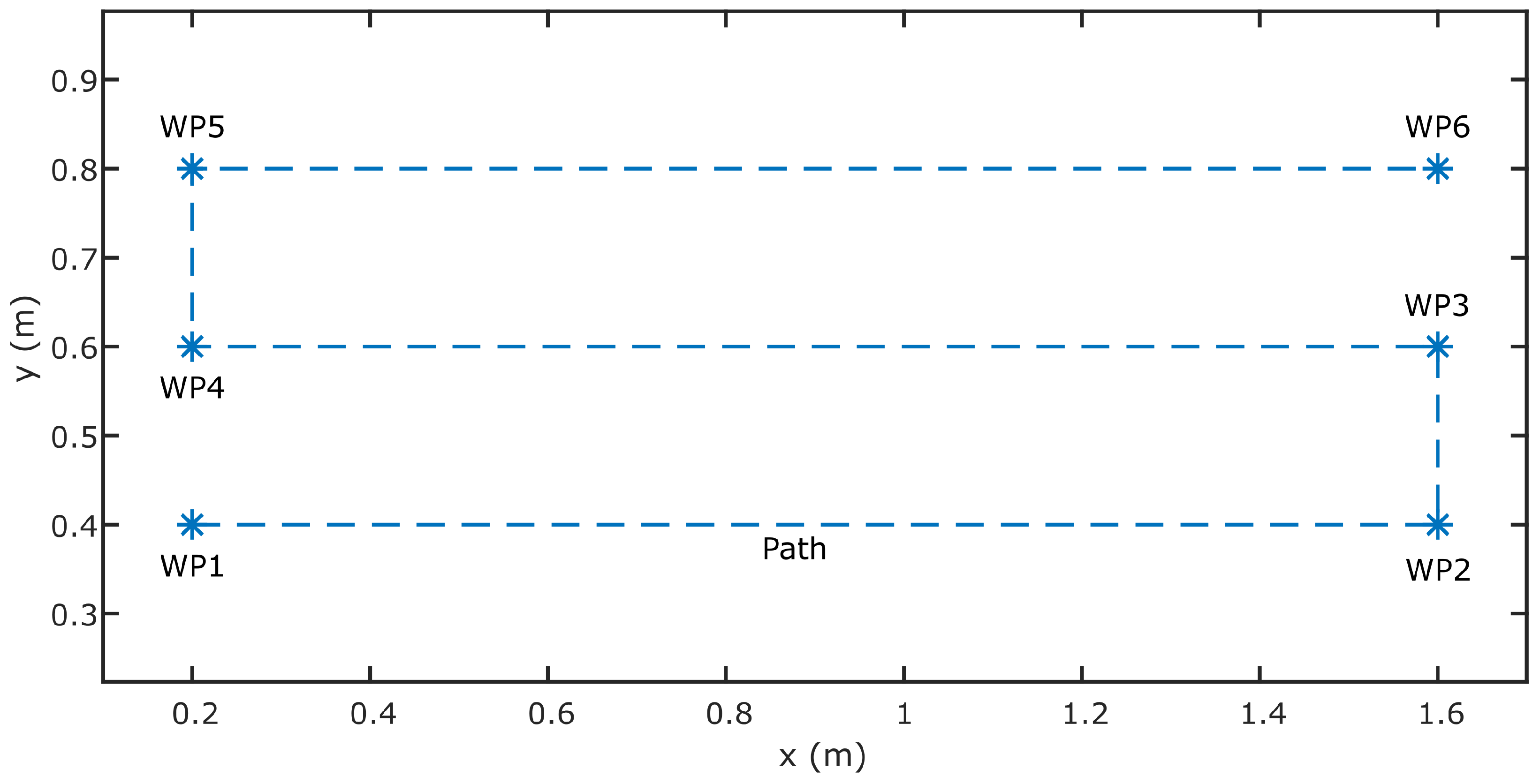
3.3.2. Global Planner

The global planner is used to produce waypoints that the robot navigates between. The planner discussed below is an example that has been designed to meet the requirements of the application discussed in Section 1.2.1. However, the design of the global planner is application dependent and should be changed or replaced to best meet the requirements of the task. Since the environment is static, waypoints can be positioned prior to inspection commencing and no replanning is necessary. In most circumstances, environments that mobile robots operate in have nonuniform cost maps due to the presence of obstacles or asymmetry of the 2D environment [33]. For the present case, the 2D environment is rectangular and has no obstacles, meaning that a cost map is unnecessary. For this reason, the environment can be covered efficiently with a boustrophedon path [34]. The stripe gap, yaw angle and rectangular area to be covered are the inputs to the boustrophedon global path planner and the output is a 2D array of waypoints. Figure 6 shows the x and y coordinates that are produced by a typical usage of the global planner. Yaw is fixed and remains constant for each waypoint.

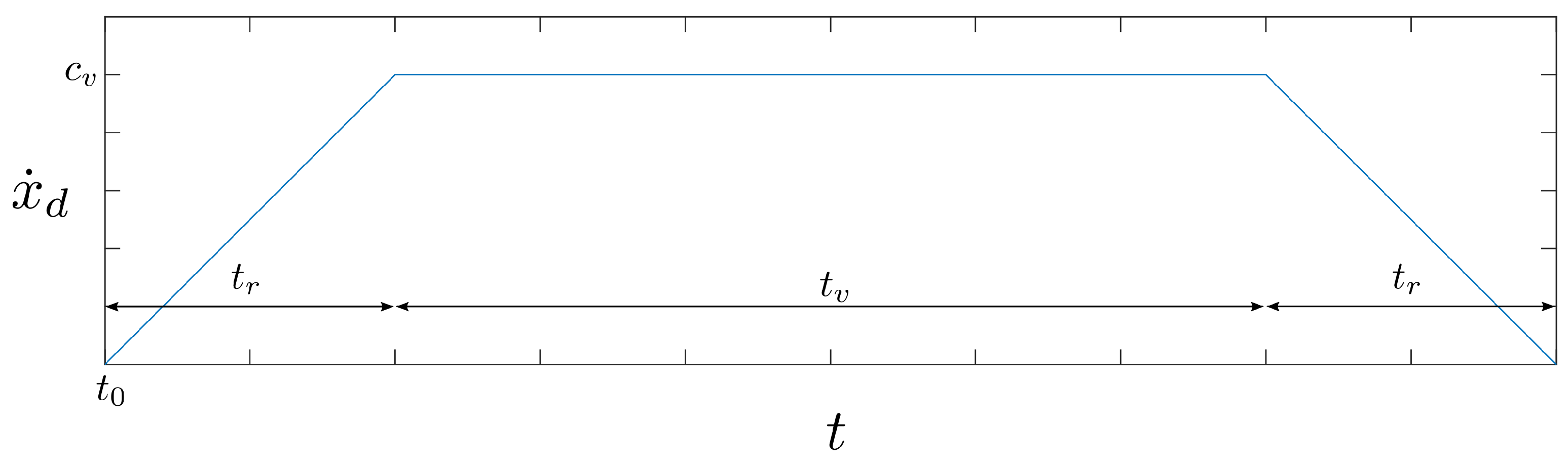
3.3.3. Local Planner

The local planner is responsible for calculating the desired poses and velocities required for MallARD to travel between two waypoints as a function of time s d t . Since MallARD is fully actuated in its degrees of freedom and there are no dynamic obstacles in the environment, there is no need for the local planner to deform the initial global plan to account for the kinematic model of the vehicle or to avoid obstacles [35]. As such, the planner plots a straight line between the start pose η s and the goal pose η g and ramps the velocities of the vehicle ( x ˙ , y ˙ , ψ ˙ ) from zero at a given acceleration c a to a maximum velocity c v and back down to zero again for its arrival at the goal pose. In the following explanation of the local planner, x is used as the target parameter but the same algorithm is used for y and ψ and so the equations are omitted for brevity.
With reference to Figure 7, when new goal x g and zero x s poses are sent to the local planner, the current time t is recorded and set as t 0 , t r and t v are calculated as follows:
t r = c v x c a x ,
t v = Δ x t r c v x c v x ,
where Δ x = x g x s . Now, each time the loop in Figure 4 runs, the requested position and velocity x d t and x ˙ d t are calculated. The value of x ˙ d t is read directly from the function that is used to generate the plot in Figure 7 and x d t is found by integration of the plot function between t 0 and t.

3.3.4. Trajectory Tracking Controller

The trajectory tracking controller is responsible for holding MallARD on the path dictated by the local planner. For aquatic and aerial vehicles alike, there is no direct means of controlling velocity at a low level as one might control the velocity of a wheel on a ground robot. For this reason, it is necessary to implement a trajectory tracking controller that interfaces with the higher level localisation systems to stop the vehicle drifting off its trajectory due to the presence of external disturbances or imbalances in physical components [7,36,37].
The trajectory tracking controller takes inputs from the local planner, s d = η d η ˙ d = x d , y d , ψ d , x d ˙ , y d ˙ , ψ d ˙ T ; the SLAM algorithm, η = x , y , ψ T and the numerical differentiation algorithm η ˙ = x ˙ , y ˙ , ψ ˙ T and outputs the propulsion force/moment vector in the navigation frame τ n = X , Y , Ψ T . It is important to note that τ n and τ b are not real forces but are analogous to force because the relationship between the force output and PWM input to the thruster’s ESCs is close to linear. The units of τ n and τ b are arbitrary as they are affected by the control parameters.
The trajectory controller consists of three PD position controllers:
X = x d x k p x + x ˙ d x ˙ k v x ,
Y = y d y k p y + y ˙ d y ˙ k v y ,
Ψ = ψ d ψ k p ψ + ψ ˙ d ψ ˙ k v ψ ,
where k p x , k v x , k p y , k v y , k p ψ , k v ψ are tuneable control parameters.

3.3.5. Localisation and Mapping

When the MallARD is placed in the pool and initialised, LiDAR scans start being delivered to the SLAM algorithm: Hector mapping [29]. MallARD is then manually driven around the pool using the joypad while the SLAM algorithm builds a complete and accurate map. With a complete map, MallARD is ready to begin autonomous navigation. At this point the SLAM algorithm is essentially performing localisation as the map remains virtually constant.

3.3.6. Numerical Differentiation

The velocity components of the state vector at index i ( x ˙ i , y ˙ i , ψ ˙ i ) are computed in real-time by numerical differentiation using current and previous readings of the displacement components ( x i , y i , ψ i ), where i is the index of the main loop as presented in Figure 4. Equation (8) gives the algorithm in terms of x, however, the algorithm is identical for y and ψ therefore their equations are once again omitted for brevity.
x ˙ i = j = i n d 1 i x j x j 1 t j t j 1 n d
Throughout the present work n d = 4 .

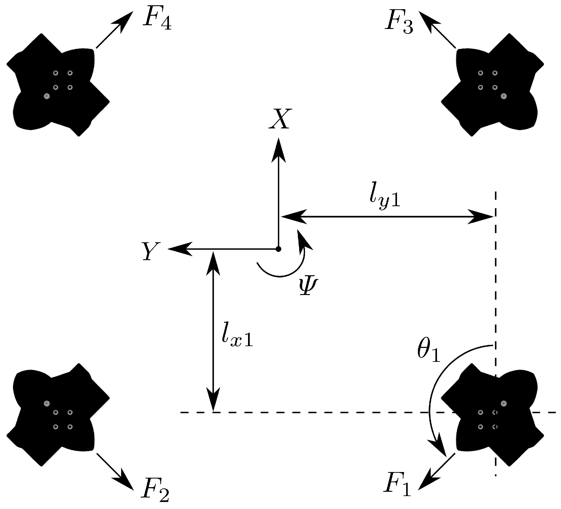
3.3.7. Thrust Allocation

The trajectory tracking controller outputs the propulsion demand force/moment vector τ n = X , Y , Ψ T in the navigation frame and is converted to τ b in the body frame using Equation (1). The relationship between control demand and individual actuator demand is given by:
τ b = T τ t ,
where T is the thrust allocation matrix and τ t = F 1 , F 2 , F 3 , F 4 T is the vector of individual actuator demands. With reference to Figure 8, T is formed by considering the contribution of each thruster to each component of τ n , i.e.,
T = cos θ 1 sin θ 1 l y 1 cos θ 1 l x 1 sin θ 1 cos θ 2 sin θ 2 l y 2 cos θ 2 l x 2 sin θ 2 cos θ 3 sin θ 3 l y 3 cos θ 3 + l x 3 sin θ 3 cos θ 4 sin θ 4 l y 4 cos θ 4 + l x 4 sin θ 4 T .
Since τ t is required in terms of τ b Equation (9) must be rearranged,
τ t = T τ b
where, T is the Moore-Penrose inverse of T .
For the present system, l x 1 = l x 2 = l x 3 = l x 4 = 0.15 m , l y 1 = l y 2 = l y 3 = l y 4 = 0.205 m , θ 1 = 3 / 4 π rad, θ 2 = 5 / 4 π rad, θ 3 = 1 / 4 π rad and θ 4 = 7 / 4 π rad.

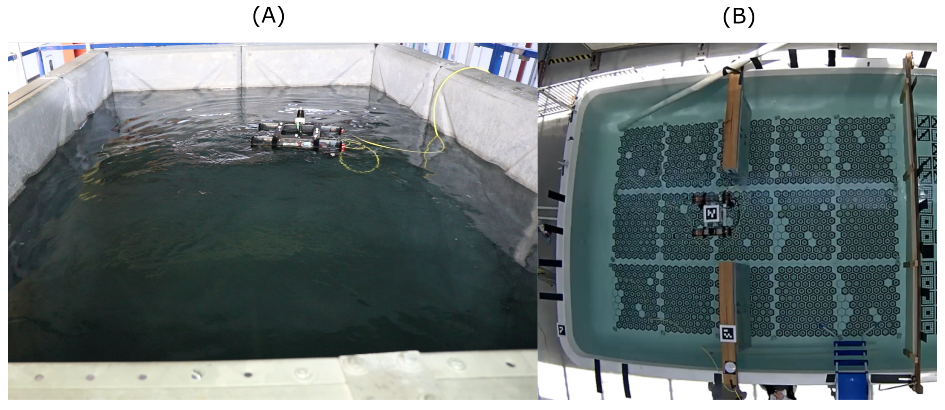
4. Experiments and Deployments

4.1. Experiment Setup
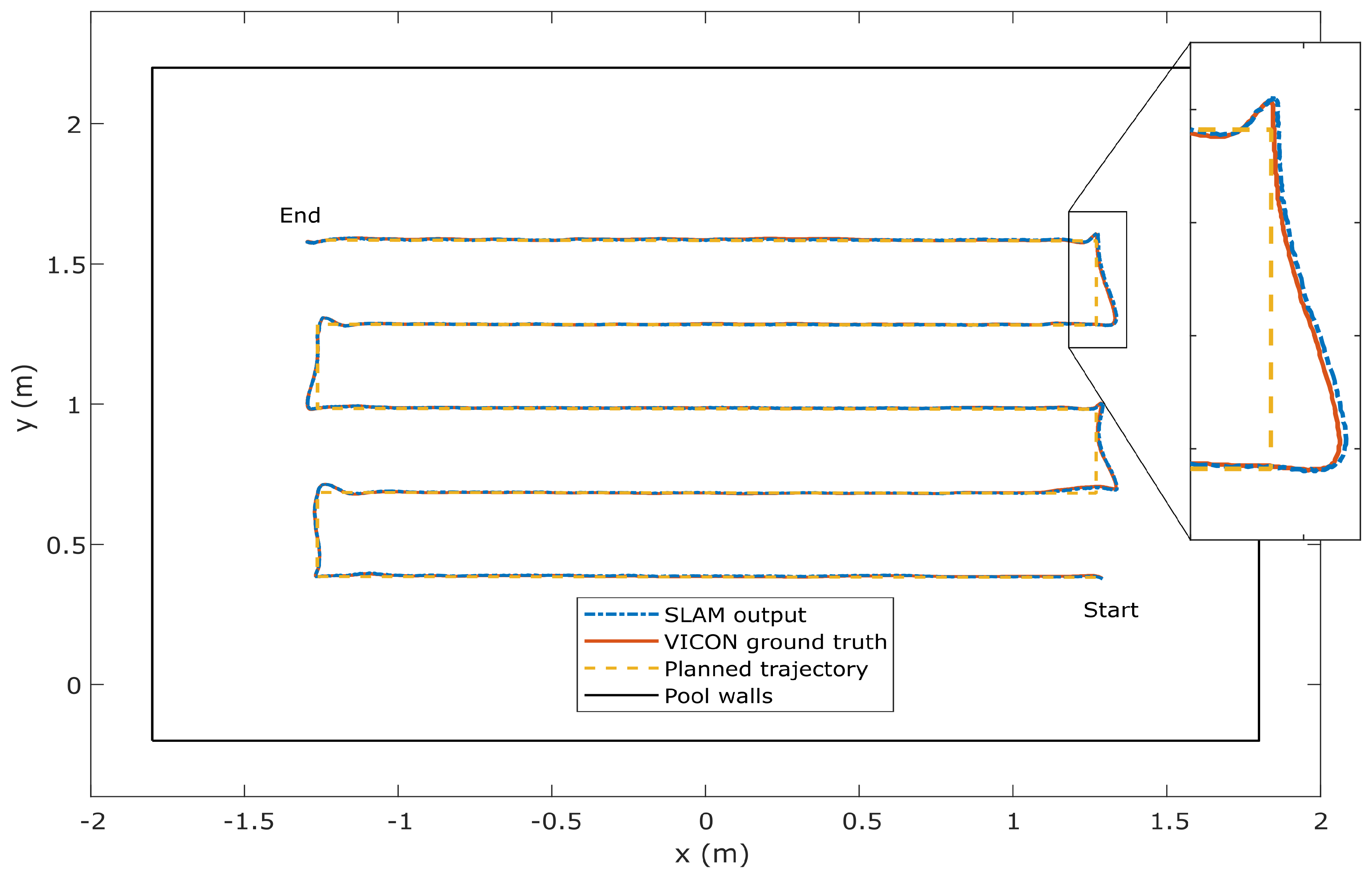
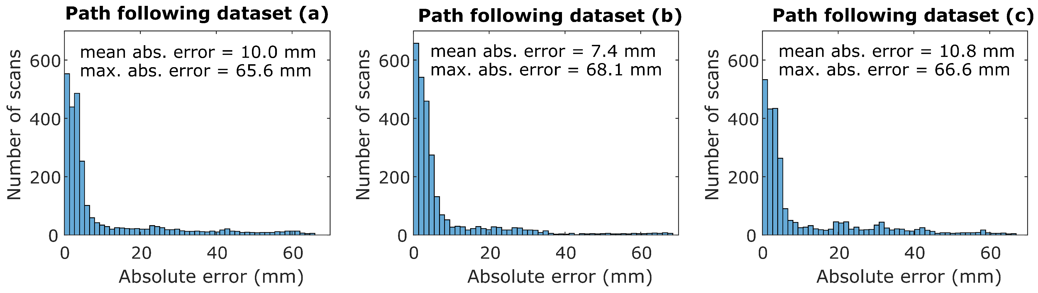
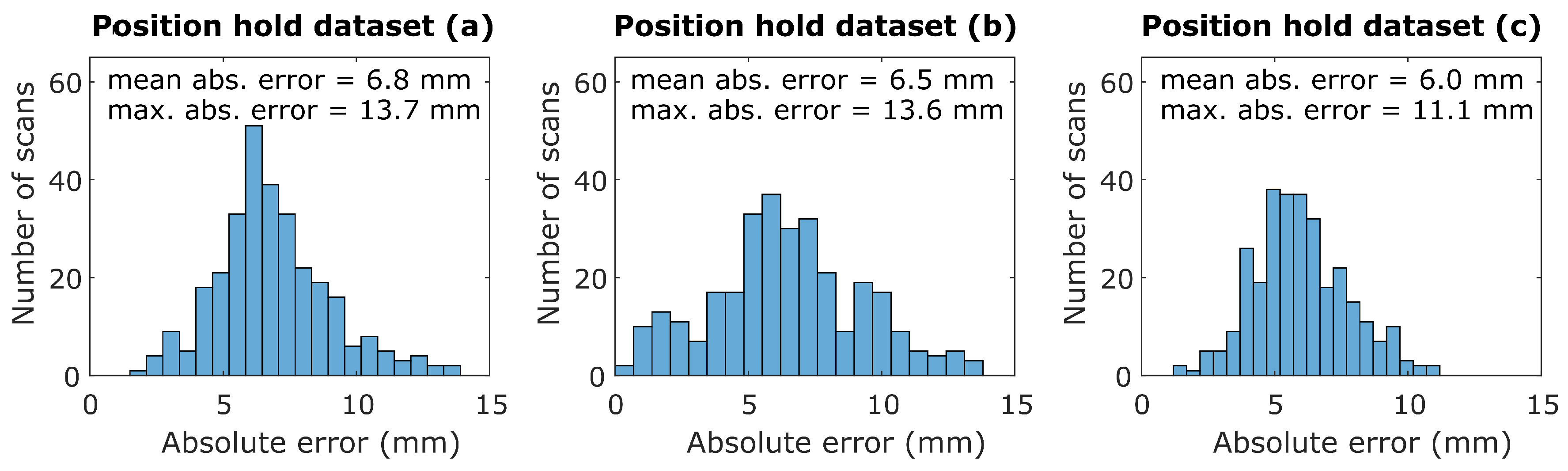
The functional localisation and control accuracy of the MallARD platform has been tested in two experiments that were designed to mimic the two application examples discussed in Section 1.2.1 and Section 1.2.2. Figure 9A shows the MallARD in the tank at the University of Manchester’s test facility where the experiments were performed. The control gains were tuned individually for each of the three degrees of freedom to give the fastest return to a set-point possible while restricting visible overshoot to two oscillations. This tuning method is repeatable and gives a good balance between stability, tracking performance and tolerance to external forces such as wind, currents and tether interaction. During testing the only significant source of external disturbance was the tether. While the tether is flexible and manually fed out as the robot requires, it still causes a significant disturbance that is difficult to quantify. In all testing the linear and angular velocity limits on ASV were set to 0.1 m/s and 0.2 rad/s respectively and the stripe gap was set to 0.3 m.
Experiment one assessed the accuracy of the MallARD when following a stripe path (Figure 6) in a 2.35 m by 3.58 m test pool. The motion pattern used in this test is representative of the motion path that would be required of MallARD when deploying an ICVD, as per Section 1.2.1. For this experiment, the global planner described in Section 3.3.2 was used to set out waypoints and the desired yaw was always set to zero. The experiment was repeated three times.
In experiment two, the MallARD platform’s ability to repeatably move to the same fixed pose near to a wall and hold the pose was tested. Returning to a known position and holding a pose is the type of behaviour that might be required for deploying a radiation sensor, as described in Section 1.2.2. In this experiment, the global planer was bypassed and pose goals were sent directly to the local planner. Once a goal was reached the robot is programmed to hold its pose. After 20 seconds holding the pose, the MallARD was sent to an arbitrary position in the pool before being sent back to hold the same initial pose again for 20 s. MallARD was sent from an arbitrary pose to the initial pose near a wall three times.

4.2. Results

Figure 10 shows the measured and planned trajectory of the ASV for the first run of experiment one. The trajectory of the robot is measured onboard by the LiDAR and associated SLAM algorithm. For the duration of the experiments, MallARD’s dynamic pose was also measured by a VICON motion capture system consisting of 12 cameras mounted around the pool. The VICON measurement was used as a ground truth to verify the accuracy of the SLAM output as well as the full system accuracy. The accuracy of the VICON system has been shown to be sub-millimetre in representative testing [38] and this was confirmed by the system’s internal error calculation metric. As is apparent in Figure 10, the output from the SLAM algorithm and the VICON system match very closely. The overall RMS error between the VICON system and the SLAM output in the x and y directions over the three experiments was 1.9 mm.
Figure 11 presents the trajectory error for the three runs of experiment one. Trajectory error is measured at each time index (in the 15 Hz loop) as the Euclidean distance between the local planner’s x , y position request and the VICON measured x , y position. Figure 12 shows the error spread for the three 20-s-long position holding tests performed in experiment two. Additionally presented in Figure 11 and Figure 12 is the mean absolute trajectory error and maximum absolute trajectory error for each test.

4.3. Deployments

In addition to the experiments performed in a lab setting, the MallARD has been used in two trial deployments carrying a mock Cherenkov viewing device [2], with the goal of automating spent fuel verification tasks. The first deployment was in Brisbane, Australia (Figure 9B) in a pool with features representative of a SFP including strong water pumps and obstacles; MallARD performed the prescribed task well, holding trajectory with confidence in the presence of strong disturbances. The second deployment was in a real SFP in Finland where the robot was again successfully deployed, this time the MallARD was deployed by trained IAEA operatives without assistance from University of Manchester researchers.

5. Discussion and Future Work

For the path tracking experiments, Figure 10 and Figure 11 show that when the ASV is following a straight line, the absolute error is very low < 10 mm. This meets the application requirements of sub-centimetre path tracking accuracy set out in Section 1.2.1. However, as might be expected, when the vehicle makes a sharp change in direction the error spikes and remains high for a few seconds until the vehicle settles on the next straight path. This error spike will not significantly degrade the system performance as tracking accuracy is only critical when following lines of fuel.
When compared to previous ASVs in the literature [6,7,8,9], the tracking error achieved by the MallARD is around two orders of magnitude lower. However, it must be noted that this comparison is somewhat unfair because the MallARD is a unique ASV designed for an application that is quite dissimilar to any previously published works. It is perhaps more appropriate to consider the present work a benchmark for the development of similar systems in the future.
In the position holding experiments (Figure 12) the MallARD also performed well, with absolute errors generally below one centimetre despite the disturbance of the tether. This proves that the MallARD platform is suitable for deploying radiation sensors and holding them in repeatable positions near walls.
Now that the MallARD platform is fully functional and its capabilities have been quantified in baseline experiments, there are many options for using it in further research. During development and testing, two potentially significant sources of error were identified and will be the subject of future work. First, common to all electric motors, the thrusters used on MallARD have a deadband around zero. Due to the relatively low thrust requirements of the system in comparison to the capacity of the thrusters, the deadband may have a considerable impact on the effectiveness of the control system. With the current thruster layout, it is possible to avoid the deadband altogether by only allowing the motors to spin in one direction and having all thrusters spinning even when the ASV is still. Second, compared to the pose reading from the VICON system, the reading from the SLAM algorithm is noisy. Therefore, to produce a smooth velocity reading via numerical differentiation, a long time history is required, meaning there is a trade-off between noise on the velocity reading and latency. It may be possible to remove the latency and significantly reduce noise by fusing the SLAM output with an IMU or dynamic system model, improving the performance of the control system by improving the accuracy and precision of its inputs.
Other areas of research that are planned for the MallARD platform include: Evaluating and optimising MallARD’s ability to track trajectories with known quantifiable disturbances present; using MallARD in collaboration with an underwater vehicle to provide accurate localisation of the submersible without additional external infrastructure; implementing model predictive control on MallARD to improve trajectory tracking ability; auto-tuning of system model coefficients and replacing elements of the software system, such the dynamic system model, with neural networks.

6. Conclusions

A novel autonomous surface vehicle (ASV) that is capable of aiding the automation of inspection and monitoring tasks in spent fuel pools (SFPs) and wet silos has been presented. A variety of sensors were evaluated with consideration made to the environmental and operational conditions. The performance of the vehicle’s localisation system, path tracking accuracy and position holding accuracy were investigated in a series of experiments and validated against a robust ground truth. The localisation system was found to have an average of error of under 2 mm and the path tracking and position holding error was approximately 1 cm, whereas previous vehicle’s mean path tracking error is 1 m or above. The drastic reduction in tracking error is down to two key factors: First, the present vehicle uses a 2D LiDAR for localisation which gives much higher accuracy and refresh rates than previous vehicles that were designed for use outdoors in large bodies of water and used satellite triangulation as their primary method of absolute localisation; second, unlike previous systems, the present vehicle is holonomic which improves controllability significantly. A restriction of the present system is that pool sizes are limited to the range of the LiDAR used and the pool must be surrounded by vertical walls that protrude at least 0.3 m above the water surface. The unique ASV platform detailed and benchmarked in this paper is highly adaptable and is ready to be used for further research into improvements in localisation and control of aquatic vehicles in confined environments.

Author Contributions

Conceptualization, K.G. (Keir Groves), A.W., J.C. and B.L.; Data curation, K.G. (Keir Groves), K.G. (Konrad Gornicki) and B.L.; Formal analysis, K.G. (Keir Groves), K.G. (Konrad Gornicki) and J.C.; Funding acquisition, K.G. (Keir Groves), S.W., J.C. and B.L.; Investigation, K.G. (Keir Groves) and K.G. (Konrad Gornicki); Methodology, K.G. (Keir Groves), A.W., J.C. and B.L.; Project administration, S.W. and B.L.; Resources, B.L.; Software, K.G. (Keir Groves) and A.W.; Supervision, J.C. and B.L.; Validation, K.G. (Keir Groves), K.G. (Konrad Gornicki) and B.L.; Visualization, A.W.; Writing—original draft, K.G. (Keir Groves); Writing—review & editing, K.G. (Keir Groves), A.W., S.W. and J.C.

Funding

This research was funded by by the Engineering and Physical Sciences Research Council under grants: EP/P01366X/1, EP/P018505/1 and EP/R026084/1.

Acknowledgments

The authors thank Jennifer Jones for assistance with project management and Vlad Hondru for his contribution to software development.

Conflicts of Interest

The authors declare no conflict of interest.

References

  1. Joyce, M. Nuclear Engineering: A Conceptual Introduction to Nuclear Power; Butterworth-Heinemann: Oxford, UK, 2017. [Google Scholar]
  2. IAEA. Safeguards Techniques and Equipment; Number 1 (Rev. 2) in International Nuclear Verification Series; International Atomic Energy Agency: Vienna, Austria, 2011. [Google Scholar]
  3. Peehs, M.; Fleisch, J. LWR Spent Fuel Storage Behaviour. J. Nucl. Mater. 1986, 137, 190–202. [Google Scholar] [CrossRef]
  4. Mallios, A.; Ridao, P.; Ribas, D.; Hernandez, E. Scan matching SLAM in underwater environments. Auton. Robot. 2014, 36, 181–198. [Google Scholar] [CrossRef]
  5. Yacout, A. Nuclear Fuel; Technical Report; Argonne National Laboratory: Lemont, IL, USA, 2011.
  6. Balbuena, J.; Quiroz, D.; Song, R.; Bucknall, R.; Cuellar, F. Design and implementation of an USV for large bodies of fresh waters at the highlands of Peru. In Proceedings of the OCEANS 2017-Anchorage, Anchorage, AK, USA, 18–21 September 2017; pp. 1–8. [Google Scholar]
  7. Dunbabin, M.; Grinham, A. Experimental evaluation of an autonomous surface vehicle for water quality and greenhouse gas emission monitoring. In Proceedings of the IEEE International Conference on Robotics and Automation (ICRA), Anchorage, AK, USA, 3–7 May 2010; pp. 5268–5274. [Google Scholar]
  8. Melo, M.; Mota, F.; Albuquerque, V.; Alexandria, A. Development of a robotic airboat for online water quality monitoring in lakes. Robotics 2019, 8, 19. [Google Scholar] [CrossRef]
  9. Griffith, S.; Pradalier, C. Survey Registration for Long-Term Natural Environment Monitoring. J. Field Robot. 2016, 34, 188–208. [Google Scholar] [CrossRef]
  10. Conte, G.; De Capua, G.P.; Scaradozzi, D. Modeling and control of a low-cost ASV. IFAC Proc. Vol. 2012, 45, 429–434. [Google Scholar] [CrossRef]
  11. Liu, Z.; Zhang, Y.; Yu, X.; Yuan, C. Unmanned surface vehicles: An overview of developments and challenges. Annu. Rev. Control 2016, 41, 71–93. [Google Scholar] [CrossRef]
  12. Monteiro, L.S.; Moore, T.; Hill, C. What is the accuracy of DGPS? J. Navig. 2005, 58, 207–225. [Google Scholar] [CrossRef]
  13. Ramezani, M.; Khoshelham, K.; Fraser, C. Pose estimation by Omnidirectional Visual-Inertial Odometry. Robot. Auton. Syst. 2018, 105, 26–37. [Google Scholar] [CrossRef]
  14. Munguía, R.; Urzua, S.; Bolea, Y.; Grau, A. Vision-based SLAM system for unmanned aerial vehicles. Sensors 2016, 16, 372. [Google Scholar] [CrossRef]
  15. Fuentes-Pacheco, J.; Ruiz-Ascencio, J.; Rendón-Mancha, J.M. Visual Simultaneous Localization and Mapping: A Survey. Artif. Intell. Rev. 2015, 43, 55–81. [Google Scholar] [CrossRef]
  16. Bristeau, P.J.; Callou, F.; Vissiere, D.; Petit, N. The navigation and control technology inside the ar. drone micro uav. IFAC Proc. Vol. 2011, 44, 1477–1484. [Google Scholar] [CrossRef]
  17. Niu, X.; Yu, T.; Tang, J.; Chang, L. An Online Solution of LiDAR Scan Matching Aided Inertial Navigation System for Indoor Mobile Mapping. Mob. Inf. Syst. 2017, 2017, 4802159. [Google Scholar] [CrossRef]
  18. Massot-Campos, M.; Oliver-Codina, G. Optical sensors and methods for underwater 3D reconstruction. Sensors 2015, 15, 31525–31557. [Google Scholar] [CrossRef] [PubMed]
  19. Ryu, J.H.; Gankhuyag, G.; Chong, K.T. Navigation system heading and position accuracy improvement through GPS and INS data fusion. J. Sens. 2016, 2016, 7942963. [Google Scholar] [CrossRef]
  20. Tang, J.; Chen, Y.; Niu, X.; Wang, L.; Chen, L.; Liu, J.; Shi, C.; Hyyppa. LiDAR scan matching aided inertial navigation system in GNSS-denied environments. Sensors 2015, 15, 16710–16728. [Google Scholar] [CrossRef] [PubMed]
  21. Travis, W.; Simmons, A.T.; Bevly, D.M. Corridor navigation with a LiDAR/INS Kalman filter solution. In Proceedings of the Intelligent Vehicles Symposium, Las Vegas, NV, USA, 6–8 June 2005; pp. 343–348. [Google Scholar]
  22. Alonge, F.; D’Ippolito, F.; Garraffa, G.; Sferlazza, A. A hybrid observer for localization of mobile vehicles with asynchronous measurements. Asian J. Control 2019. [Google Scholar] [CrossRef]
  23. Mallios, A. Sonar Scan Matching for Simultaneous Localization and Mapping in Confined Underwater Environments. Ph.D. Thesis, University of Girona, Girona, Spain, 2014. [Google Scholar]
  24. Newman, P.; Leonard, J.J.; Rikoski, R. Towards constant-time SLAM on an autonomous underwater vehicle using synthetic aperture sonar. In Proceedings of the International Symposyum of Robotics Research (ISRR03), Siena, Italy, 19–22 October 2003. [Google Scholar]
  25. Mallios, A.; Ridao, P.; Ribas, D.; Maurelli, F.; Petillot, Y. EKF-SLAM for AUV navigation under probabilistic sonar scan-matching. In Proceedings of the 2010 IEEE/RSJ International Conference on Intelligent Robots and Systems, Taipei, Taiwan, 18–22 October 2010; pp. 4404–4411. [Google Scholar]
  26. Ribas, D.; Ridao, P.; Tardós, J.D.; Neira, J. Underwater SLAM in man-made structured environments. J. Field Robot. 2008, 25, 898–921. [Google Scholar] [CrossRef] [Green Version]
  27. Arnold, S.; Medagoda, L. Robust Model-Aided Inertial Localization for Autonomous Underwater Vehicles. In Proceedings of the 2018 IEEE International Conference on Robotics and Automation (ICRA), Montreal, QC, Canada, 21–26 May 2018. [Google Scholar]
  28. Hegrenaes, O.; Hallingstad, O. Model-aided INS with sea current estimation for robust underwater navigation. IEEE J. Ocean. Eng. 2011, 36, 316–337. [Google Scholar] [CrossRef]
  29. Kohlbrecher, S. Hector Slam; Technical Report; Open Source Robotics Foundation: Mountain View, CA, USA, 2016. [Google Scholar]
  30. Lennox, C.; Groves, K.; Hondru, V.; Arvin, F.; Gornicki, K.; Lennox, B. Embodiment of an Aquatic Surface Vehicle in an Omnidirectional Ground Robot. In Proceedings of the 2019 IEEE International Conference on Mechatronics (ICM), Ilmenau, Germany, 18–20 March 2019. [Google Scholar]
  31. Foote, T.; Purvis, M. REP 103 Standard Units of Measure and Coordinate Conventions; Technical Report; Open Source Robotics Foundation: Mountain View, CA, USA, 2014. [Google Scholar]
  32. Fossen, T.I. Guidance and Control of Ocean Vehicles; Wiley: New York, NY, USA, 1994. [Google Scholar]
  33. Ferguson, D.; Stentz, A. Field D*: An Interpolation-Based Path Planner and Replanner. In Robotics Research; Thrun, S., Brooks, R., Durrant-Whyte, H., Eds.; Springer: Berlin/Heidelberg, Germany, 2007; pp. 239–253. [Google Scholar] [Green Version]
  34. Choset, H.; Pignon, P. Coverage path planning: The boustrophedon cellular decomposition. In Field and Service Robotics; Springer: Berlin, Germany, 1998; pp. 203–209. [Google Scholar]
  35. Marin-Plaza, P.; Hussein, A.; Martin, D.; Escalera, A.d.l. Global and local path planning study in a ros-based research platform for autonomous vehicles. J. Adv. Transp. 2018, 2018, 6392697. [Google Scholar] [CrossRef]
  36. Yang, Y.; Du, J.; Liu, H.; Guo, C.; Abraham, A. A trajectory tracking robust controller of surface vessels with disturbance uncertainties. IEEE Trans. Control Syst. Technol. 2013, 22, 1511–1518. [Google Scholar] [CrossRef]
  37. Hoffmann, G.; Waslander, S.; Tomlin, C. Quadrotor helicopter trajectory tracking control. In Proceedings of the AIAA Guidance, Navigation and Control Conference and Exhibit, Honolulu, HI, USA, 18–21 August 2008; p. 7410. [Google Scholar]
  38. Merriaux, P.; Dupuis, Y.; Boutteau, R.; Vasseur, P.; Savatier, X. A study of vicon system positioning performance. Sensors 2017, 17, 1591. [Google Scholar] [CrossRef] [PubMed]
Figure 1. A spent fuel pool at the San Onofre Nuclear Generating Station, California.
Robotics 08 00047 g001
Figure 2. The MallARD platform design, dimensions and components.
Robotics 08 00047 g002
Figure 3. MallARD electronic connection flowchart.
Robotics 08 00047 g003
Figure 4. Flowchart describing MallARD’s localisation and autonomous navigation system structure.
Robotics 08 00047 g004
Figure 5. Earth-fixed n and body-fixed b reference frames.
Robotics 08 00047 g005
Figure 6. Output of the global planner for a rectangle defined by coordinates x 1 = 0.2 , y 1 = 0.4 , x 2 = 1.6 , y 2 = 0.8 and with a stripe gap of 0.2 m.
Robotics 08 00047 g006
Figure 7. Plot of the local planner’s velocity ramping function, desired velocity x ˙ d t against time t.
Robotics 08 00047 g007
Figure 8. Thruster layout and notation, θ angles are measured anticlockwise from the body-fixed x-axis, lengths l are always positive.
Robotics 08 00047 g008
Figure 9. Photographs of MallARD during lab testing at The University of Manchester, UK (A) and while being deployed in a representative pool in Brisbane, Australia (B).
Robotics 08 00047 g009
Figure 10. MallARD planned trajectory, simultaneous location and mapping (SLAM) output and ground truth in the x and y axes.
Robotics 08 00047 g010
Figure 11. Histograms showing the error spread for the three repeated path tracking experiments. The absolute error is measured as the minimum Euclidean distance between the planned trajectory and the VICON measured location for each time index.
Robotics 08 00047 g011
Figure 12. Histograms showing the error spread for the three repeated position holding experiments. The absolute error is measured as the minimum Euclidean distance between the requested holding position and the VICON measured location for each time index.
Robotics 08 00047 g012
Table 1. Summary of relevant localisation technologies; data from references of Section 2.1.
TechnologyScopeMean ErrorRefresh RateEnvironmental Influence
GNSSAbsolute localisation≈1 m [12]20–50 HzOnly available outdoors
Computer visionAbsolute localisation or odometry--Highly sensitive to environment
LiDAR SLAMAbsolute localisation3–6 mm [20]≈10–50 HzRequires local features
6-axis IMUFuse with absolute localisation-≈50–200 HzAlmost unaffected
sonar SLAMAbsolute localisation1.9 m≈1–10 HzOnly available below surface

