Motion Planning and Reactive Control Algorithms for Object Manipulation in Uncertain Conditions ^†

Abstract

This work proposes the application of several smart strategies for object manipulation tasks. A real-time flexible motion planning method was developed to be adapted to typical in-store logistics scenarios. The solution combines and optimizes some state-of-the-art techniques to solve object recognition and localization problems with a new hybrid pipeline. The algorithm guarantees good robustness and accuracy for object detection through depth images. A standard planner plans collision-free trajectories throughout the whole task while a proposed reactive motion control is active. Distributed proximity sensors were adopted to locally modify the planned trajectory when unexpected or misplaced obstacles intervene in the scene. To implement a robust grasping phase, a novel slipping control algorithm was used. It dynamically computes the grasp force by adapting it to the actual object physical properties so as to prevent slipping. Experimental results carried out in a typical supermarket scenario demonstrate the effectiveness of the presented methods.

1. Introduction

The research work presented in this paper builds on a line of reactive planning and control approaches to the use of robots in unstructured environments. Computing a collision-free path in a cluttered environment is not an easy problem to solve; however, even though successfully solved, unavoidable uncertainties affecting both the perception system and the models, which are used to compute the reference robot motion, can lead to a likely failure in the real world. Therefore, the adoption of a reactive controller that can update the planned robot motion in real time based on perception data obtained in real time can lead to a more robust task execution.

The adoption of robots in the retail market scenario, both in distribution centers and in supermarket stores, is still far from being a reality since significant technological advancements are still required. Consider the following routine task: a large number of single misplaced items per time unit have to be fetched and carried from a trolley, where other objects are already present, to a shelving unit within narrow spaces. In current stores, the idea of introducing robots to do this kind of activity still seems far away. The reason is the limited manipulation abilities in terms of the identification of different types of objects and their safe grasping and handling.

This paper is an extended version of the conference paper [1] about the execution of pick and place tasks in a supermarket scenario. It includes additional results and discussions on the selection of the motion planning and the object detection algorithms most suitable for the application at hand. The discussion on the comparison of state-of-the-art (SoA) techniques has been expanded with various examples that better explain the non-applicability of some techniques to the object recognition and localization problems. Furthermore, two new sections are added on grasp planning and reactive control algorithms to obtain a more robust grasping phase. Section 3.2 investigates how to fix the grasping frame on the localized object by considering the symmetries of common geometrical shapes. Section 4 has been included to apply the novel slipping control algorithm, originally presented in [2], to the typical in-store logistics task of shelf refilling in a supermarket. The algorithm dynamically computes the grasp force by adapting it to the actual object physical properties, such as weight and friction, and it is not predetermined as in the previous work.

SoA motion planners are mostly based on offline sample-based algorithms: Rapidly Exploring Random Tree (RRT) [3], Probabilistic RoadMap (PRM) [4], Expansive Spaces Tree (EST) [5], and Kinematic Planning by Interior-Exterior Cell Exploration (KPIECE) [6], are some of the most commonly used tree-based planners that have been analyzed. The experimental results described in Section 5 explain the difficulty of their practical use. Planners’ random nature often causes unnatural trajectories which are impossible to predict. The common planning algorithms work in the joint space, so they need an Inverse Kinematics (IK) solver to compute the target robot configuration. Kinematic and Dynamic Solver (KDL) [7] is the most used IK solver: it is based on Newton’s method with some random jumps. However, careless use of any IK solver can produce unneeded robot reconfigurations.

Another challenging technology needed for robotic applications in the logistics domain is object recognition and 6D localization used to estimate both the position and orientation of the object to be grasped. The SoA point-cloud-based techniques propose pipelines which are difficult to generalize. Some local descriptors, such as Fast Point Feature Histograms (FPFH) [8] or Signature of Histograms of OrienTations (SHOT) [9], work well when the scene is simple, e.g., when there are few objects that are far enough from each other and of very different shapes. On the other hand, the main limit of global descriptors, such as Viewpoint Feature Histogram (VFH) [10], is that partial occlusions highly affect the result.

This paper proposes solutions to overcome some of the limitations in SoA planners. By deeply analyzing the Point Cloud Library (PCL) [11], including its algorithmic capabilities and implementation strategies [12], this research aims to find the intersection between the common global and local pipelines, to optimize them, and to robustly solve the object recognition and 6D localization problems. An efficient RANdom SAmple Consensus (RANSAC) method [13] was exploited. The result is a new hybrid pipeline, which segments the observed scene, identifies the clusters, and compares them with a point cloud representation of the target object. As in [14], such object representation is obtained by starting from a CAD. The novel contribution is from the association step: it depends not only on the comparison of descriptors but also on the alignment process itself. Even if a higher success rate can be reached, the main drawback is a longer computational time.

The second contribution consists of a procedure that avoids the execution of strange and unnatural motions by planning trajectories with no unnecessary arm reconfigurations. A specific IK solver constrains the robot joint limits to be as close as possible to the initial state.

Finally, this technology is not limited to a simple “plan and act” approach, but it reacts to uncertainties and to dynamic changes in the scene. In fact, the robot is endowed with a reactive control capability—both in the grasp, through sensorized fingers [2,15], and in the robot motion, through distributed proximity sensors [16]—and corresponding control algorithms that can adapt the planned task to the needs of the robot acting in the real world.

A series of experiments were conducted on two object sets and with an industrial robot in a setting representative of a shelf refilling task in a supermarket scenario (see Figure 1).

2. Object Recognition and Localization

The proposed object recognition and 6D localization algorithm is based on a new hybrid approach, which merges the main steps of the SoA local and global pipelines. The developed model-based algorithm processes the point cloud data acquired by the sensory system described in Section 2.1.

2.1. Sensory System

To create the depth map, a depth camera was adopted: the Intel RealSense R410 (Intel Corporation, Sabta Clara, CA, USA). The camera was used as a vision device for both object recognition and 6D localization (see Figure 1). It does not use RGB information but just an IR emitter to project a light pattern and an IR sensor to detect its deformation. The R410 maximum resolution is 1280 × 720. A point-cloud-based calibration procedure was developed to estimate both the intrinsic and extrinsic parameters of the camera according to the camera position criteria explained in Section 2.3.4. The procedure generates two homogeneous transformation matrices by using a fixed coordinate frame on a corner of a reference object: $T_{object}^{robot}$, which expresses the pose of the object frame with respect to the robot base frame, $T_{object}^{camera}$, which expresses the pose of the object frame with respect to the camera frame. By combining them, the $T_{camera}^{robot}$ matrix can be extracted.

2.2. Modeling of the Object Set

The first data set of objects used to broadly test the quality of the detection algorithms is shown in Figure 2a: they are purposely different in terms of size and shape. The final set of objects used for the training process is shown in Figure 2b, which contains objects geometrically more similar to each other. This set is designed to stress the algorithm and test its robustness.

Since no 3D models were directly available for the selected objects, many of them were reconstructed automatically using the Intel sensor and the ReconstructMe software [17] that generates a CAD-model of the object. For the objects of simple geometry, the CAD-model was directly drawn using a CAD program in STL format. Views of the resulting CAD-models can be seen in Figure 3. Note that ReconstructMe is not able to distinguish transparent, thin, and polished objects. Therefore, some objects were excluded from the set (those not labeled in Figure 2b). All the CAD-models were finally converted into Point Cloud Models (PC-models), to be elaborated by PCL.

2.3. Comparison with Existing Algorithms

The heart of a common recognition algorithm is the 3D data matching process. This step is done by comparing two point sets, $S_1$ and $S_2$, through a method based on the descriptor notion, as explained in [1]. Descriptors can be defined as being like structures that contain useful information to summarize the points of a point cloud, and they are used to search for correspondences between the PC-model and the perceived object. As described in [12], depending on the way they represent the information, 3D descriptors can be divided into two main categories: signatures or histograms. The descriptor of each category can be local or global, in accordance with the extension of the point cloud to which it is applied. Figure 4 shows two possible standard pipelines. However, some limitations have been found to the application of the SoA approaches to different cases study. To overcome these difficulties, a new hybrid pipeline was adopted.

2.3.1. Local Pipeline

Referring to Figure 4, the local pipeline uses local descriptors, which work on key-points. These special points describe a specific neighborhood, defined by a fixed radius from its center. The description of a complete object consists of associating each point with a descriptor of the local geometry of the same point. Tests carried out with edge extraction, a typical key-point criterion, did not produce satisfactory results in cluttered scenes.

The second difficulty was the definition of the support size value, which is used to determine the subset of neighboring points around each key-point. This choice greatly influences the characterization of the local descriptor. The parameter may be defined either in terms of distance radius or in terms of the number of neighbors. A critical trade-off emerged during experimental tests: if the support size is too small, the descriptor will describe basic features like planes and corners and will lose its ability to discriminate. On the other hand, if the support size is too large, it will contain information from much of the background and it will not match to anything.

A third critical parameter to choose was the optimal threshold value to use for the correspondence step: too low a value generates too many possible poses of the PC-model in the scene; too high a value makes the matching algorithm too greedy, because it does not find any overlaps between the PC-model and the scene.

Tuning these values to work well in different cases study was impossible, as better described in Section 2.3.4.

2.3.2. Global Pipeline

With reference to Figure 4, global pipelines use global descriptors. These descriptors are high-dimensional representations of the geometric features of an object. Due to high computational cost, they are generally calculated after a 3D segmentation step. This step is needed to identify different objects inside the scene and separate them into single point clouds. Different techniques can be used to do that, as described in [1]. The cluster is described by a global descriptor, whose main limitation is related to partial occlusions: if present, the following matching phase will likely fail.

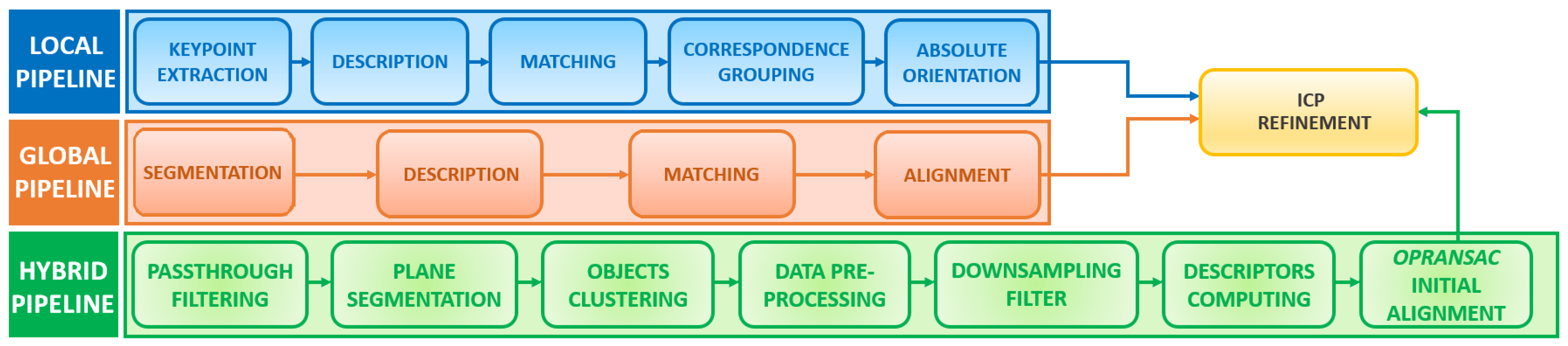
2.3.3. Hybrid Pipeline

In this specific application, the objects can be distinguished only by geometric information, without any kind of visual features (e.g., barcodes). The scene is usually large and affected by partial occlusions and similar objects in proximity. Standard recognition approaches proved to be unsuitable because of the limitations discussed above. The algorithm proposed in this paper extracts the most generalizable steps of each SoA pipeline and merges both the global segmentation and the local descriptor robustness, as shown in Figure 4. Moreover, a new approach is introduced based on the RANSAC method [13]: unlike the SoA pipeline that provides the matching phase and the alignment phase as two separated steps, the proposed algorithm performs the two phases in one step. It optimizes a critical parameter to be more efficient and robust than the traditional RANSAC approach (see Section 2.3.4). This step was called Optimized RANSAC (OPRANSAC) to underline the optimization process. The initial coarse alignment provided by OPRANSAC is finally refined by the Iterative Closest Point (ICP) method [18]. After the recognition, the algorithm output is the 6D localized pose. The hybrid pipeline is divided into eight steps:

1. PassThrough filtering. Undesirable data on the input scene are reduced by applying a series of PCL filters. Identifying the portion of the scene of interest and removing the rest can be a good way to simplify the recognition process from the beginning.

2. Plane segmentation. PCL provides Sample Consensus Segmentation (SCS), a very useful component which executes a segmentation algorithm based on normal analysis. The main problem is the choice of the right value of the parameter k, which is the number of neighbors around a point used to compute the normal vector. The RANSAC method is a randomized algorithm for robust model fitting, and SCS uses it to estimate the parameters of the mathematical plane model of the given scene. 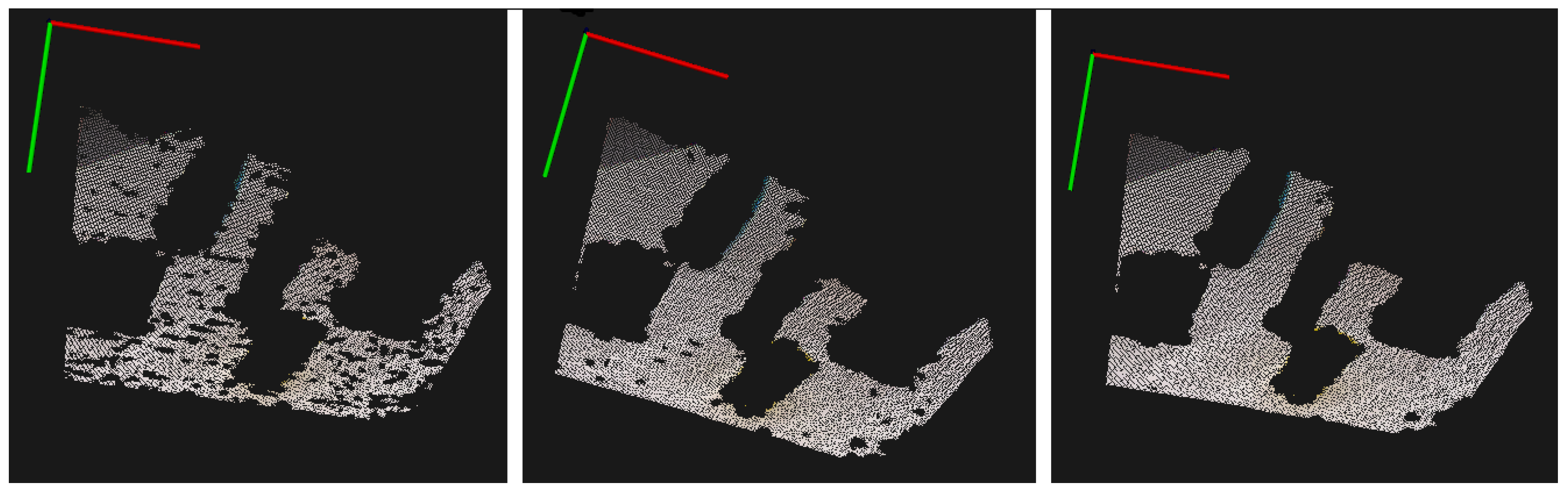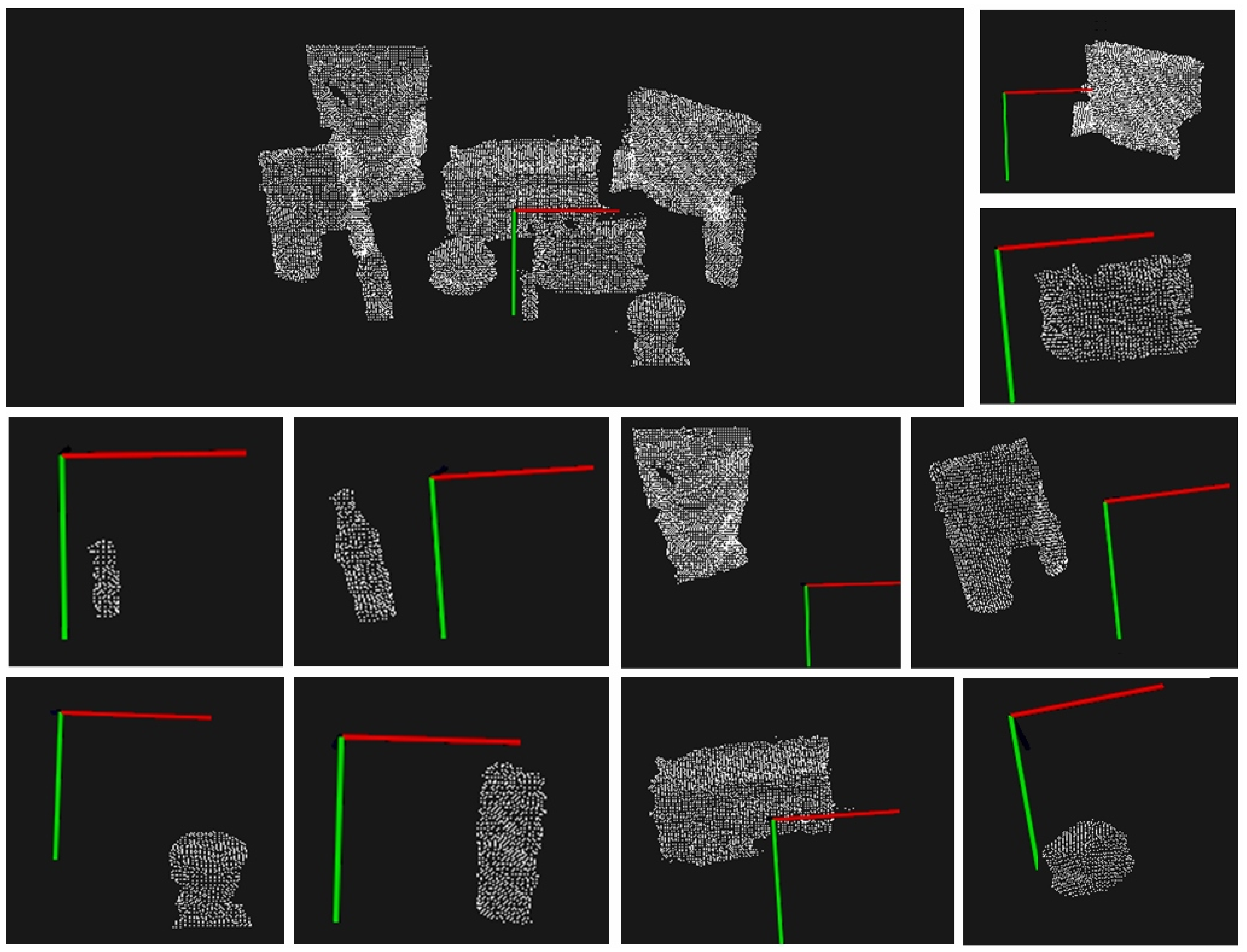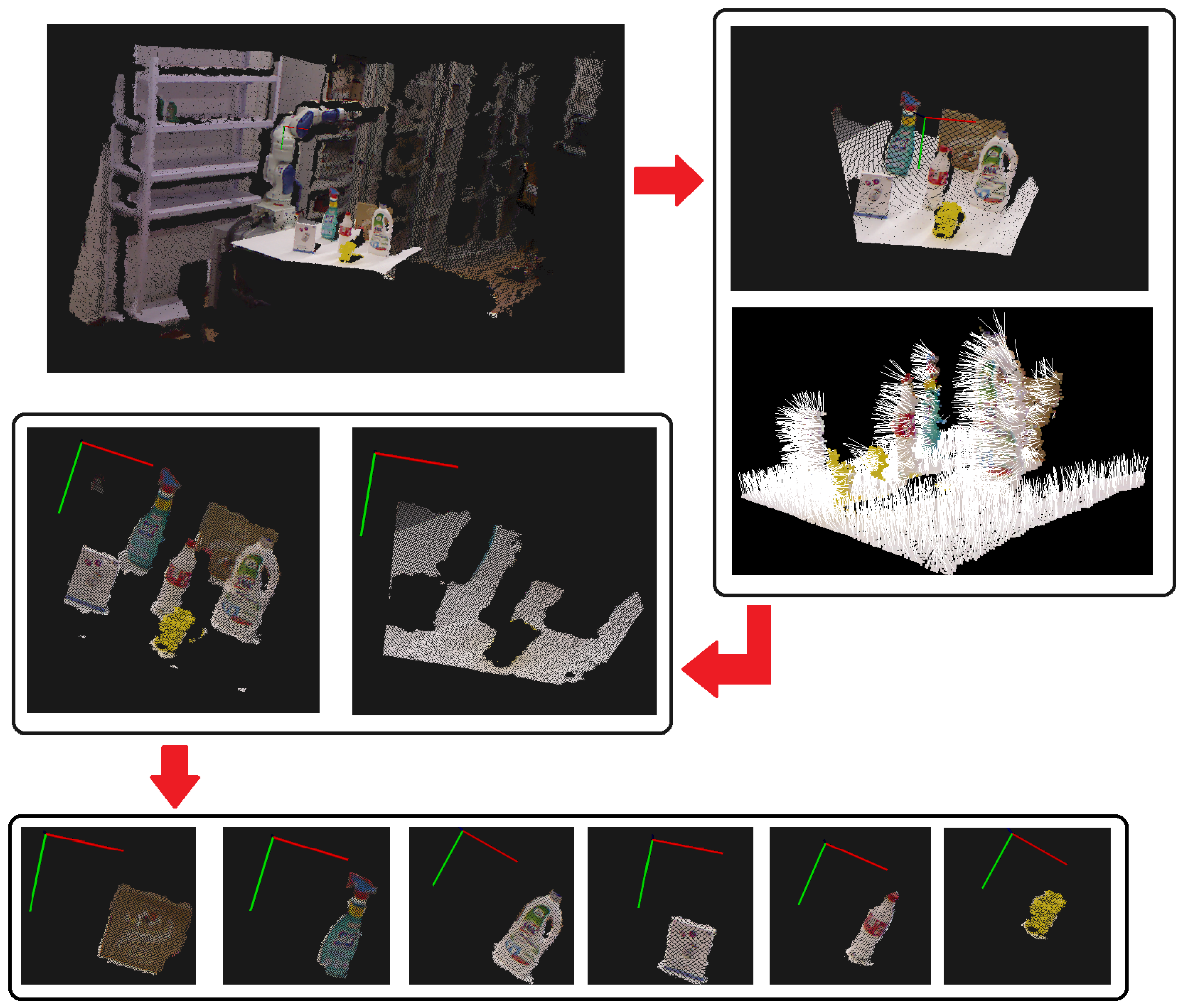RANSAC divides point data between inliers (the points which satisfy the plane equation) and outliers (all other points) by providing a vector of model coefficients. Note that extracting the plane strongly depends on the quality of the surface normals, as shown in Figure 5. The image on top-left of Figure 6 illustrates the outcome of this step.

3. Object clustering. The process is based on Euclidean Cluster Extraction (ECE) approach, which uses a Kd-tree structure to find the nearest neighbors. The method uses a fixed minimum distance threshold, $d_t$. Figure 6 shows the results.

4. Data preprocessing. Before the description analysis, each cluster and the given PC-model are passed through the Moving Least Square (MLS) filter. Overlapping areas, small registration errors, and holes are smoothed to improve the quality of the geometric descriptors.

5. VoxelGrid filter downsampling. As seen in Section 2.2, the PC-model and scene can be provided by different data sources. This means that their descriptors can be very different, and this affects the correspondence step. To improve this aspect, a simple downsampling step through a Voxelized Grid approach was used so that all point clouds have almost the same density.

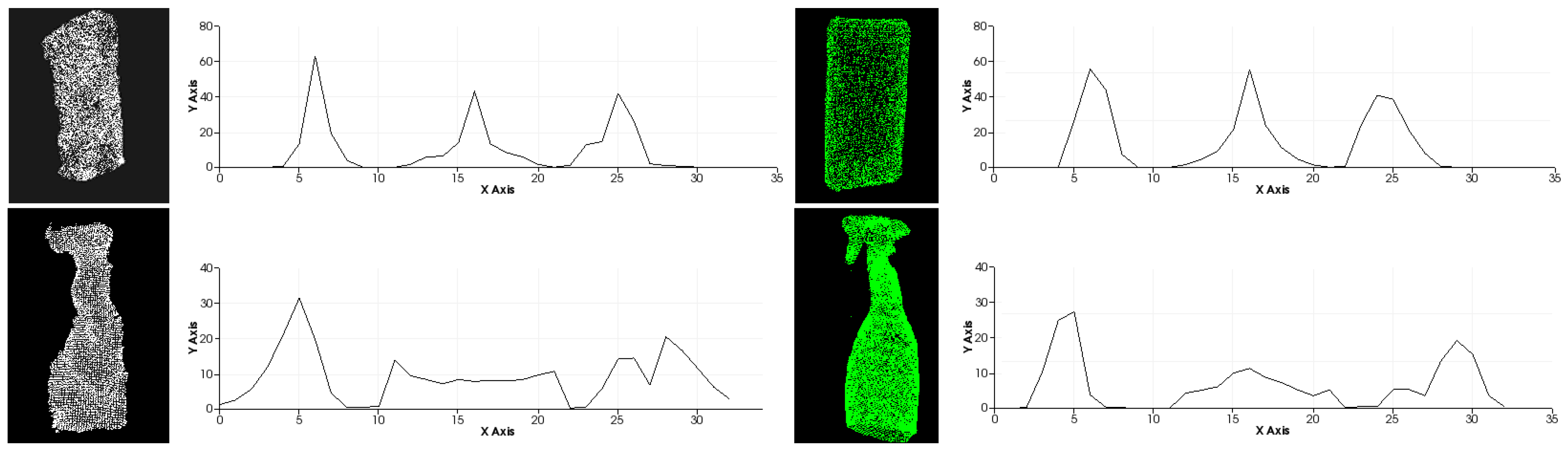
6. FPFH descriptors. The FPFH local descriptor was finally selected for its robustness after carrying out several experiments with different local and global descriptors. The main limitation of global descriptors, e.g., VFH, is that they are not suitable for complex scenarios: in the case study, there are many objects on the tray which are similar and close to each other, and very often they are occluded. FPFH features, on the other hand, represent the surface normals and the curvature of the objects, as shown in Figure 7. FPFH turned out to be the descriptor which was least influenced by the complexity of the task in most of the experimental scenarios, as described in Section 2.3.4.

7. Point cloud initial alignment: OPRANSAC. In order to compare two generic S_source and S_target point clouds in 3D space, they need to be aligned. The OPRANSAC step in Figure 4 is crucial because it must calculate the rigid geometric transformation to be applied to S_source to align it to S_target. The hybrid pipeline proposes an initial alignment obtained by following the approach in [19], i.e., by using the Prerejective RANSAC method and without having previous knowledge about the object pose. This method uses the two analyzed point clouds, the respective local FPFH descriptors, and a series of setting parameters to tune the consensus function. The alignment process was performed through the class SampleConsensusPrerejective, which implements an efficient RANSAC pose estimation loop.

The following difficulties were encountered during this phase: in some similar scenes in which the objects on the table were slightly moved, the SoA algorithm did not correctly recognize the target object, often confusing it with objects of different geometry. When it recognized the target object, the correspondence rates were very different from one scene to another or similar for different objects. So, the results obtained by these common techniques did not meet the supermarket scenario requirements. This is why a careful analysis of this crucial step was carried out: to identify only the most sensitive input parameters that affect the algorithm result. The parameter that was identified as the most critical is the number of nearest features to use ($\gamma$): small changes generate very different outputs. Trying to select a single value of this parameter for every observed scene and for every PC-model was impossible. The adopted solution is the maximization of the following fitness function over $\gamma$:

$$\begin{array}{c}[I,H]=RANSAC(S_{source},S_{target},FPF{H}_{source},FPF{H}_{target},\gamma )\hfill \end{array}$$

(1)

$$\begin{array}{c}fitness(\gamma )=\frac{\left|I\right|}{|S_{source}|},\hfill \end{array}$$

(2)

where $\left|I\right|$ is the cardinality of the set I of inlier points between the two point clouds $S_{target}$ and $S_{source}$ after the $RANSAC$ alignment calculated by using the current value of $\gamma$, and H is the 4 × 4 homogenous transformation matrix to perform such alignment. The transformation matrix $T_{OPRANSAC}^{camera}$ is extracted directly from H.

In order to assign a label to the PC-model input, a classifier was not used, but a brute force search method was adopted by selecting the label corresponding to the highest value of the fitness function. However, the fitness function value of each cluster is computed by optimizing it with respect to an algorithm parameter. To maximize the fitness function, two nested loops were implemented. The inner loop computes the best value of $\gamma$ by increasing it each time by a fixed step (i.e., ${\delta }_{\gamma }=5$). This loop represents the optimization step, and it is the core of the approach since the choice of $\gamma$ is crucial for the success of the algorithm. The external loop is just a brute force search; it executes this operation for each target cluster $S_{target}\left[j\right]$ labeled in the specific scene, i.e., with j from 1 to the number of clusters identified in the scene. Finally, the best result is chosen: the corresponding homogeneous transformation matrix and the labeled cluster are selected. The pseudo-code is reported in Algorithm 1.

Algorithm 1 OPRANSAC initial alignment.

1: input:   2: $S_{source}\leftarrow \mathrm{PC-model}\mathrm{to}\mathrm{identify}$   3: $S_{target}\leftarrow \mathrm{vector}\mathrm{of}\mathrm{all}\mathrm{labeled}\mathrm{clusters}$   4: $FPF{H}_{source}\leftarrow \mathrm{PC-model}\mathrm{descriptor}$   5: $FPF{H}_{target}\leftarrow \mathrm{descriptors}\mathrm{vector}\mathrm{of}\mathrm{labeled}\mathrm{clusters}$   6: ${\gamma }_0\leftarrow \mathrm{initial}\mathrm{value}\mathrm{of}\mathrm{the}\mathrm{critical}\mathrm{parameter}\gamma$   7: $N\leftarrow \mathrm{number}\mathrm{of}\mathrm{iterations}\mathrm{for}\mathrm{the}\mathrm{internal}\mathrm{loop}$   8: ${\delta }_{\gamma }\leftarrow \mathrm{fixed}\mathrm{step}\mathrm{for}\mathrm{the}\mathrm{critical}\mathrm{parameter}$   9: procedurePerform Alignment  10:  $fitness=0$  11:  $H=I_{4\times 4}$  12:  $label=0$  13:  for $j=1$ to $S_{target}.size$ do  14:    $\gamma ={\gamma }_0$  15:    for $i=1$ to N do  16:      $[I,H_{temp}]=RANSAC(S_{source},S_{target}\left[j\right],FPF{H}_{source},FPF{H}_{target}\left[j\right],\gamma )$  17:      $fitnes{s}_{temp}=\left|I\right|/|S_{source}|$  18:      if $fitnes{s}_{temp}>fitness$ then  19:        $fitness=fitnes{s}_{temp}$  20:        $H=H_{temp}$  21:        $label=j$  22:      end if  23:      $\gamma +={\delta }_{\gamma }$  24:    end for  25:  end for  26: end procedure

The maximum fitness value, which is equal to 1, is obtained when all the points have a near distance below the fixed ${\delta }_{th}$ threshold. The partiality of the views (clusters) and therefore of the point clouds makes unlikely a high level of fitness, although over 70% matching in the experimental tests was found. The definition of the similarity parameter, therefore, enables the comparison between incomplete object clusters and PC-models, but also it enables the definition of optimization heuristics based on the cardinality of the point clouds. 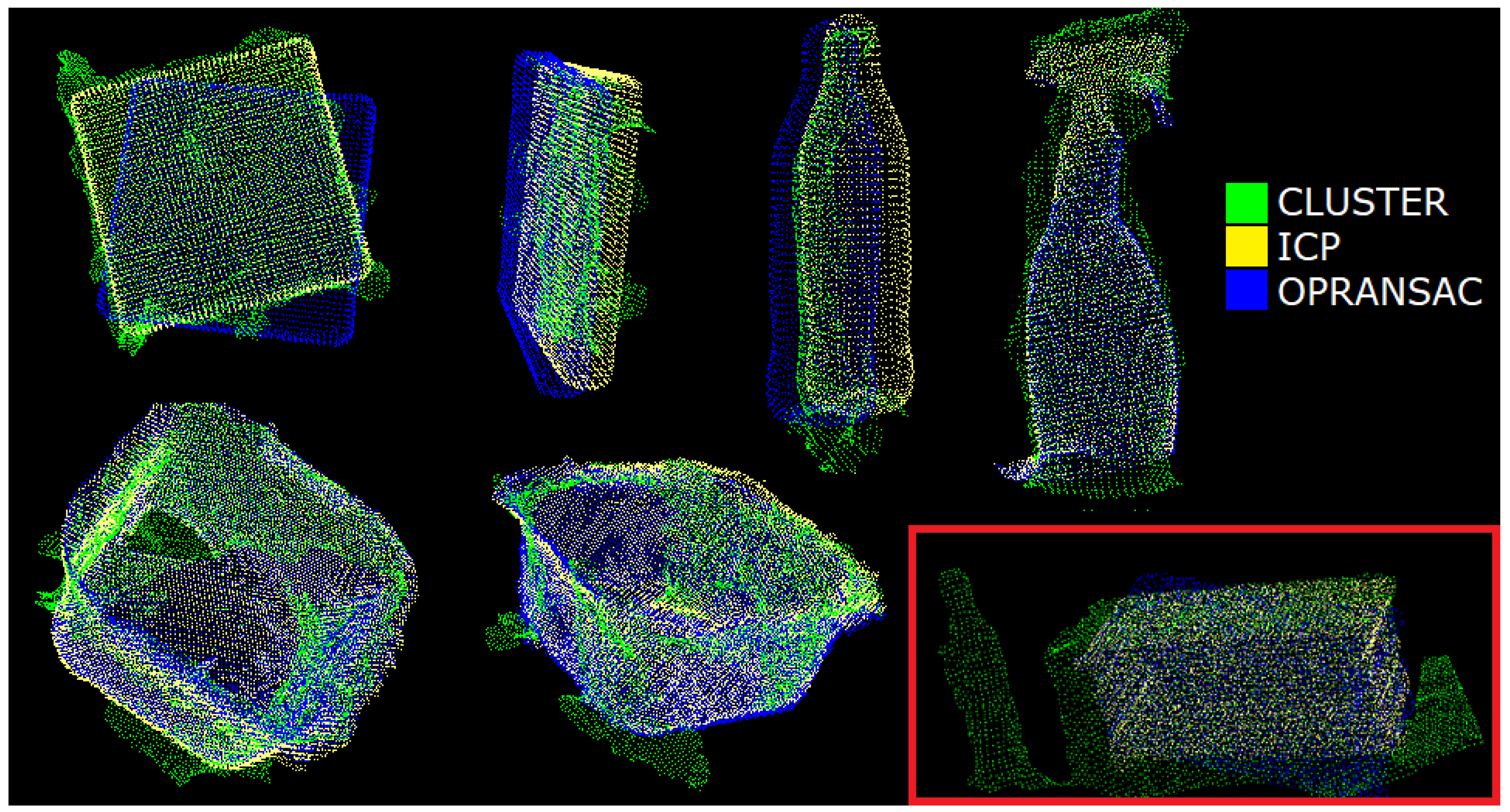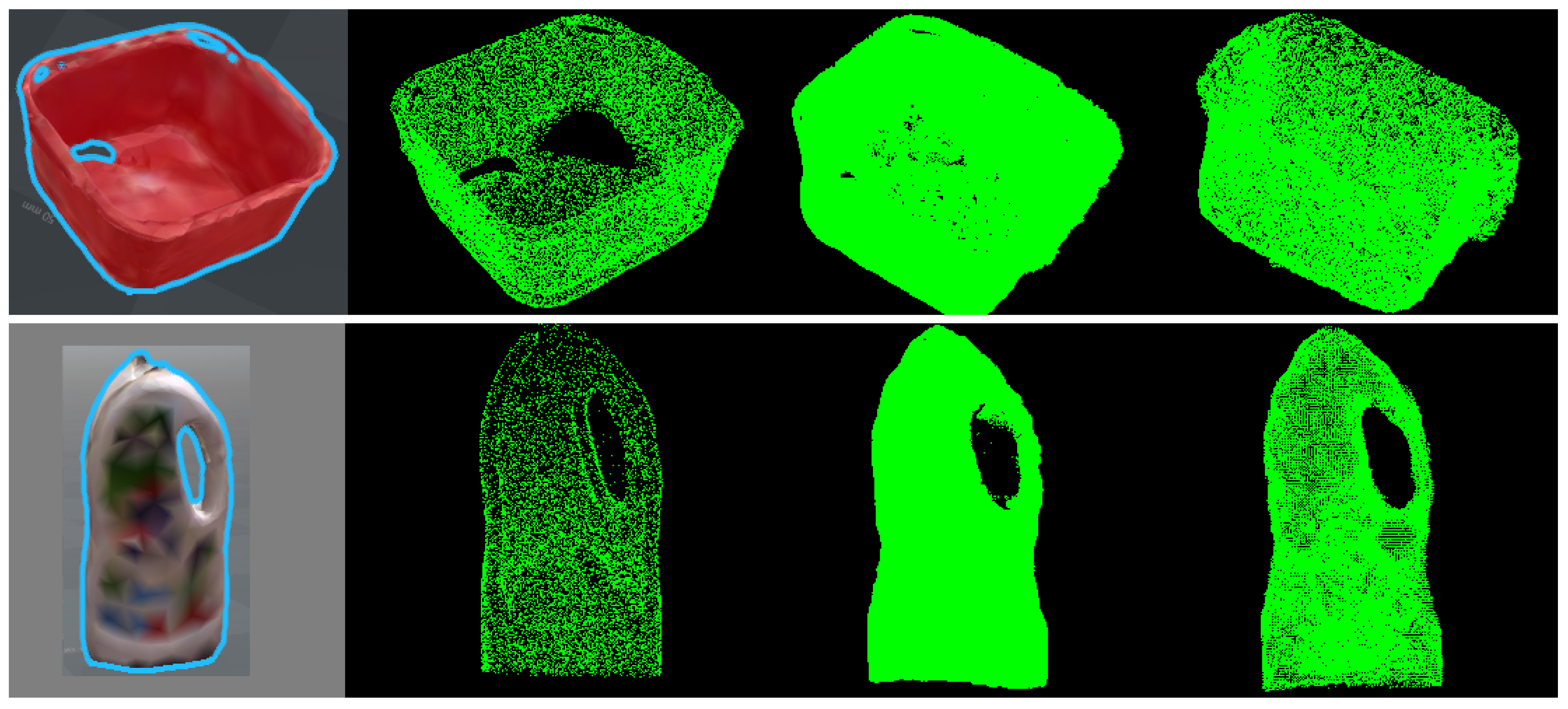Figure 8 shows some (blue) PC-models coarsely aligned to their respective (green) clusters.

8. ICP The last step of the hybrid pipeline is the ICP algorithm. $T_{OPRANSAC}^{camera}$ is refined to better estimate the 6D object pose. The output is the transformation matrix $T_{ICP}^{camera}$. Figure 8 illustrates the final result.

2.3.4. Tests and Performance Assessment

This subsection discusses the most interesting results obtained during preliminary tests carried out before the implementation of the proposed algorithm.

Camera placement. Camera placement influences the results of many recognition phases, e.g., the plane segmentation and the object clustering. When the camera is placed in a high position with respect to the object tray, the plane segmentation is good because the normals estimation is accurate. However, the clustering process becomes worse because the object front view is lost. The dimensions of both the clusters and the captured scene are influenced by the camera distance from the observed scene. The larger the distance, the smaller the object clusters, and the corresponding point clouds have fewer points. On the other hand, to frame as many objects as possible, the distance should be large enough. Finally, the distance should be high enough to let the camera stay out of the robot workspace so as to avoid an additional obstacle for the pick and place task. As a trade-off between the discussed constraints, the camera was placed such that the closest object is at about 0.3 m and the furthest one is at about 0.9 m.

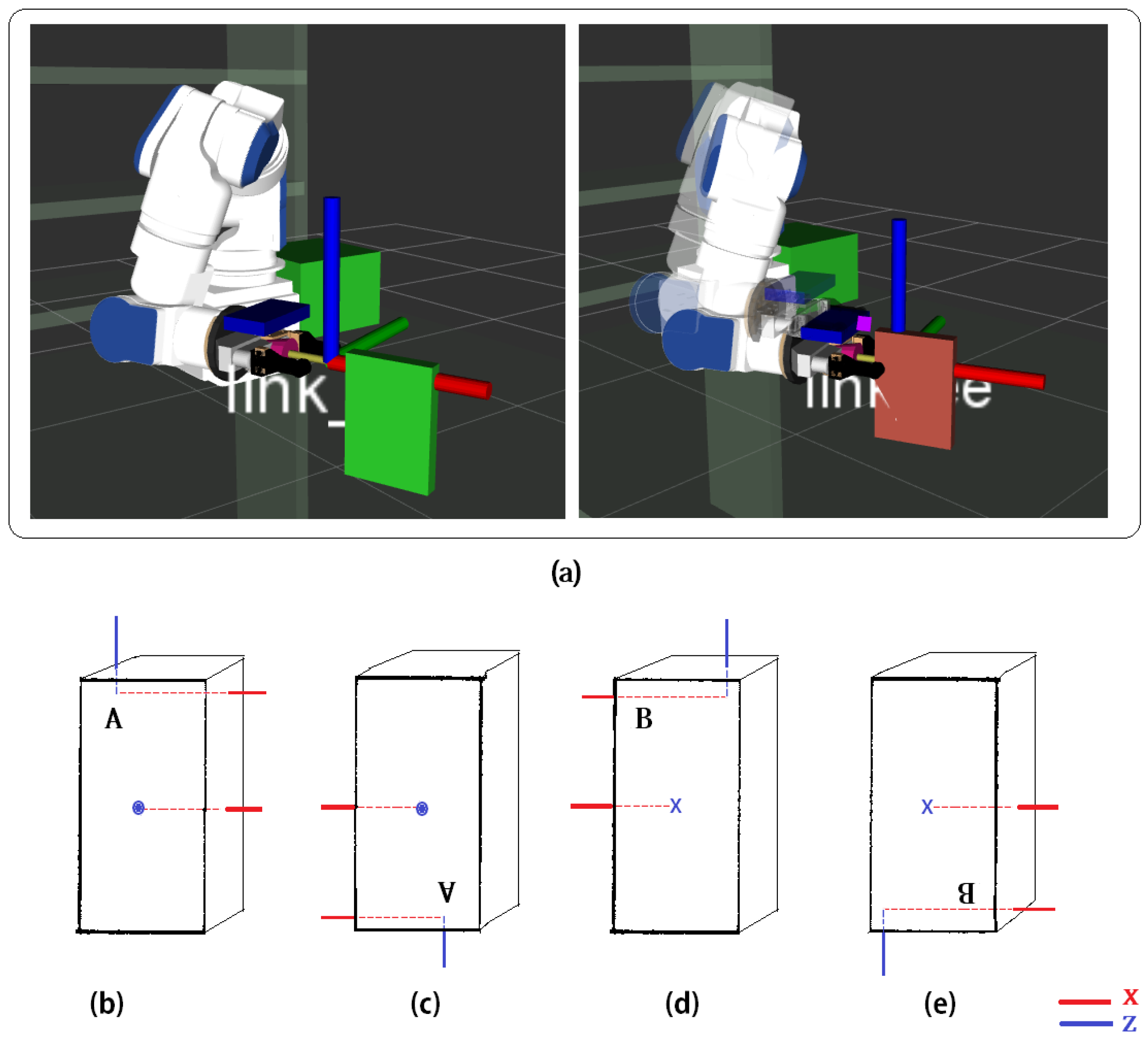
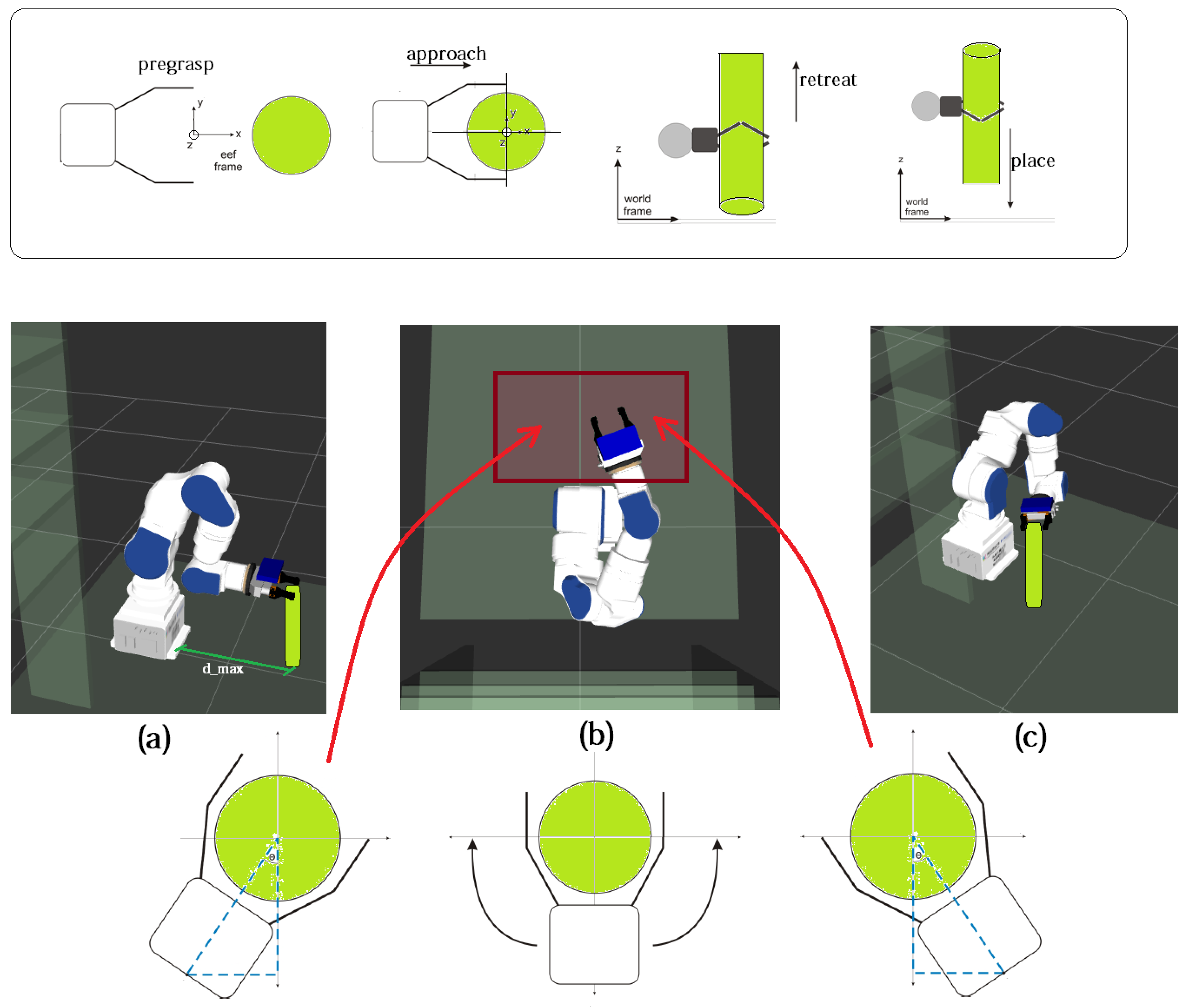
Object placement. In this work, objects are assumed to be randomly placed but all upright on the tray and at a minimum distance of 0.3 m. This value was chosen to allow the robot to grasp an object without colliding with other close objects (see Section 3.3) and also to guarantee a correct clustering of the scene. With reference to the red box in Figure 8, if the objects are closer than 0.3 m, the clustering algorithm may generate a cluster with two objects. Nevertheless, their final alignment can be still successful: the (yellow) PC-model is aligned to the correct portion of the incorrect (green) cluster.

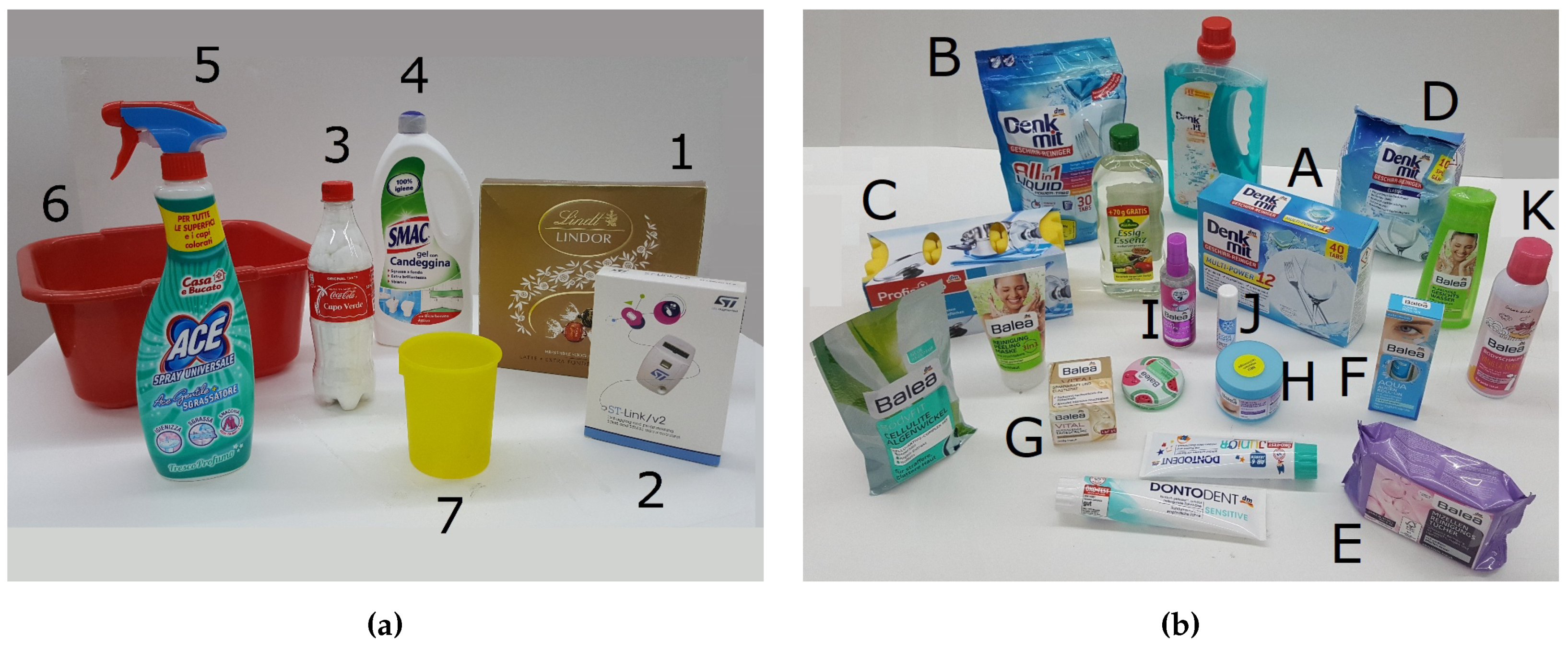
Key-point extraction tests. The first experimental tests followed step-by-step the SoA techniques based on the local pipeline applied to the first data set (Figure 2a). Referring to [20], the Normal Aligned Radial Features (NARF) algorithm deals with both the detection and the description of key-points. To the best of our knowledge, NARF is the most up-to-date and best-performing available algorithm. This method is based on two principles:

• a key-point must be placed where the surface is stable to provide a robust normal estimation, and there are also sufficient changes in the neighbors;
• if there is a partial view of the scene (like in the considered scenarios), it can focus on the edges of an object: the boundary of a foreground object will be quite unique and it can be used to extract points of interest.

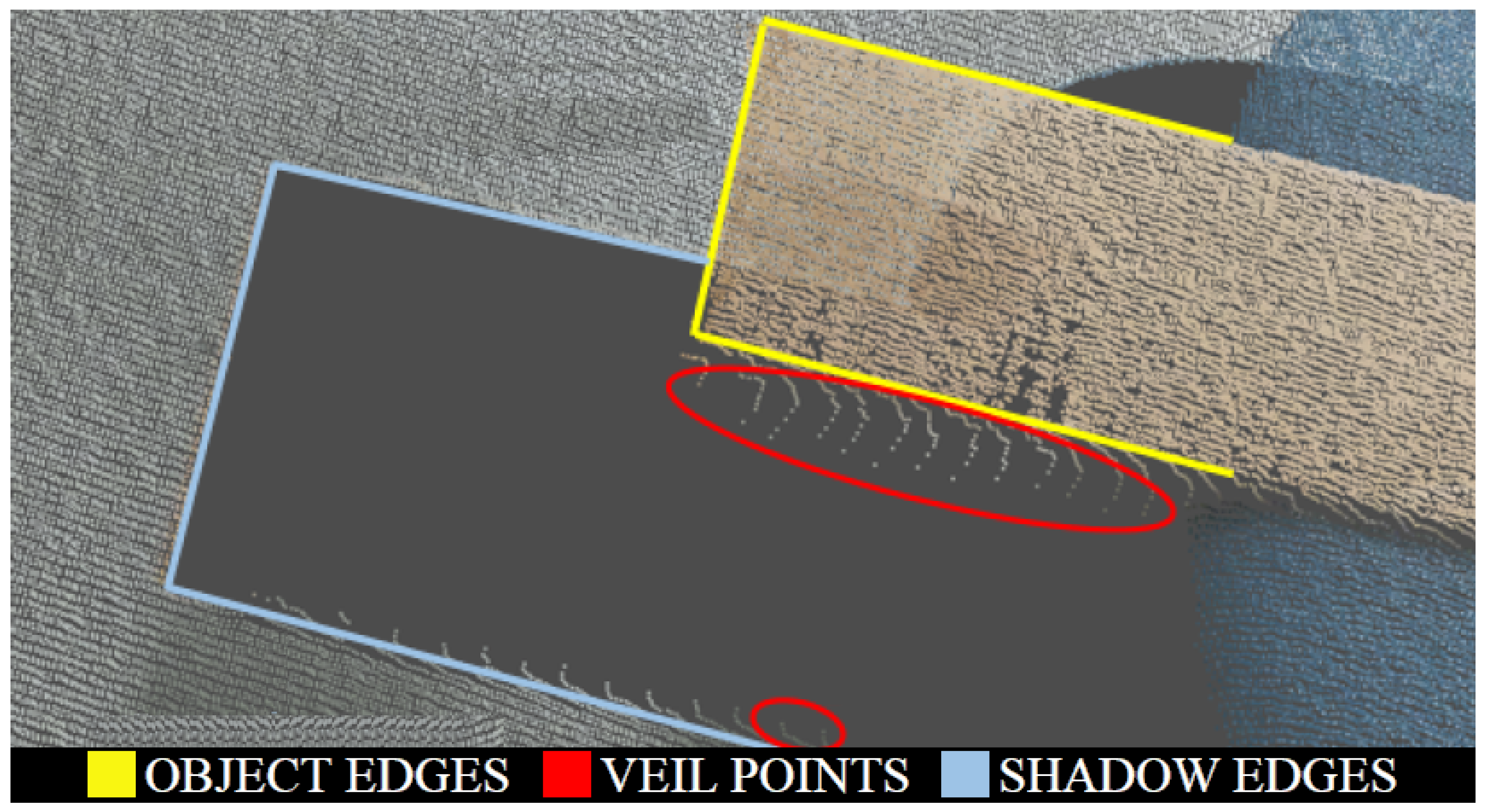
In this context, three types of interesting points can be defined, as shown in Figure 9: the Object edges, which are outer points that belong to the object, the Shaded edges, which are the background points on the boundary with occlusions, and the Veil points, which are the points interpolated between the object edges and the shadow points.

While shadow points are not useful, veil detection is required because these points should not be used during the feature extraction. There are several indicators that may be useful for edge extraction, such as critical changes of normals. NARF uses the change in the average distance of neighbors to the point, which is a very robust indicator of noise and resolution changes. This means that a good key-point needs to have significant changes in the surface around itself in order to be detected in the same place even though viewed in different perspectives.

The experimental results showed that objects that have a complex geometry (e.g., the spray bottle) give a lot of key-points (e.g., on the handle): it is possible that a detailed tuning algorithm could converge to good results. On the contrary, for the objects which have more regular geometries (e.g., the boxes), it is more difficult because too few key-points are extracted and, therefore, the percentage of failure dramatically increases when searching for model–scene correspondences.

The natural solution would be to decrease the exploration radius of the algorithm, but this alternative soon becomes a bottleneck because it extracts a greater number of key-points than the previous cases; however, many of them are fake edges. This effect is absolutely a disadvantage because the algorithm finds a number of possible combinations when it compares the PC-model and the scene, as shown in Figure 10. Choosing the right correspondence is difficult because all of them have similar matches.

A careful analysis underlines that these results also depend on other factors. For the successful adoption of a local pipeline to recognize objects, the PC-model and the scene should have the same precision, cardinality, accuracy, resolution, and scales. All of these limitations do not allow for the generalization of the use of this algorithm, especially when using PC-models extrapolated directly from some online existing databases. That is why the key-point extraction method was completely discarded.

Hybrid pipeline applied to the first data set. To evaluate the general behavior of the proposed pipeline in terms of its precision and reliability, an extensive test was initially executed on 50 different scenes containing objects of the first data set (Figure 2a).

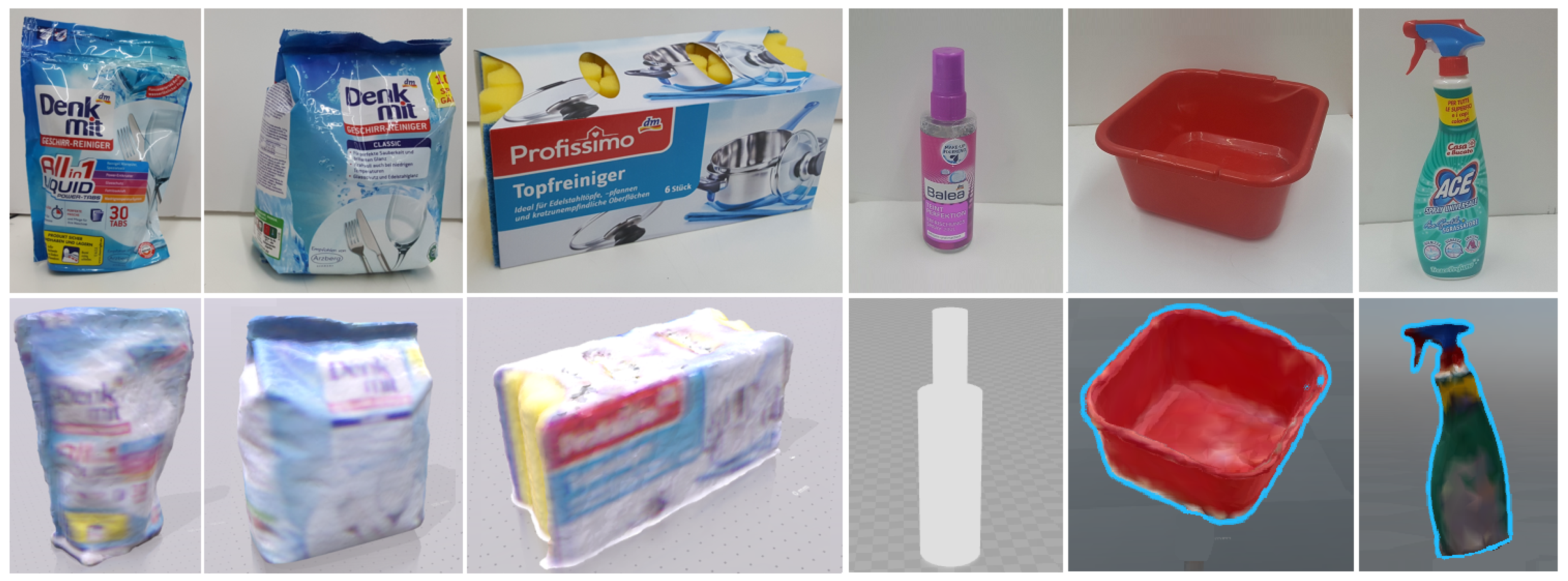
Some testing objects were reconstructed using the ReconstructMe software. Despite the rough modeling of some parts (e.g., holes in the basin or the absence of the green cap of the soap bottle), the corresponding PC-models, for a size ranging from 100 kB to 200 kB, were directly used and processed in the proposed pipeline, showing its convenience.

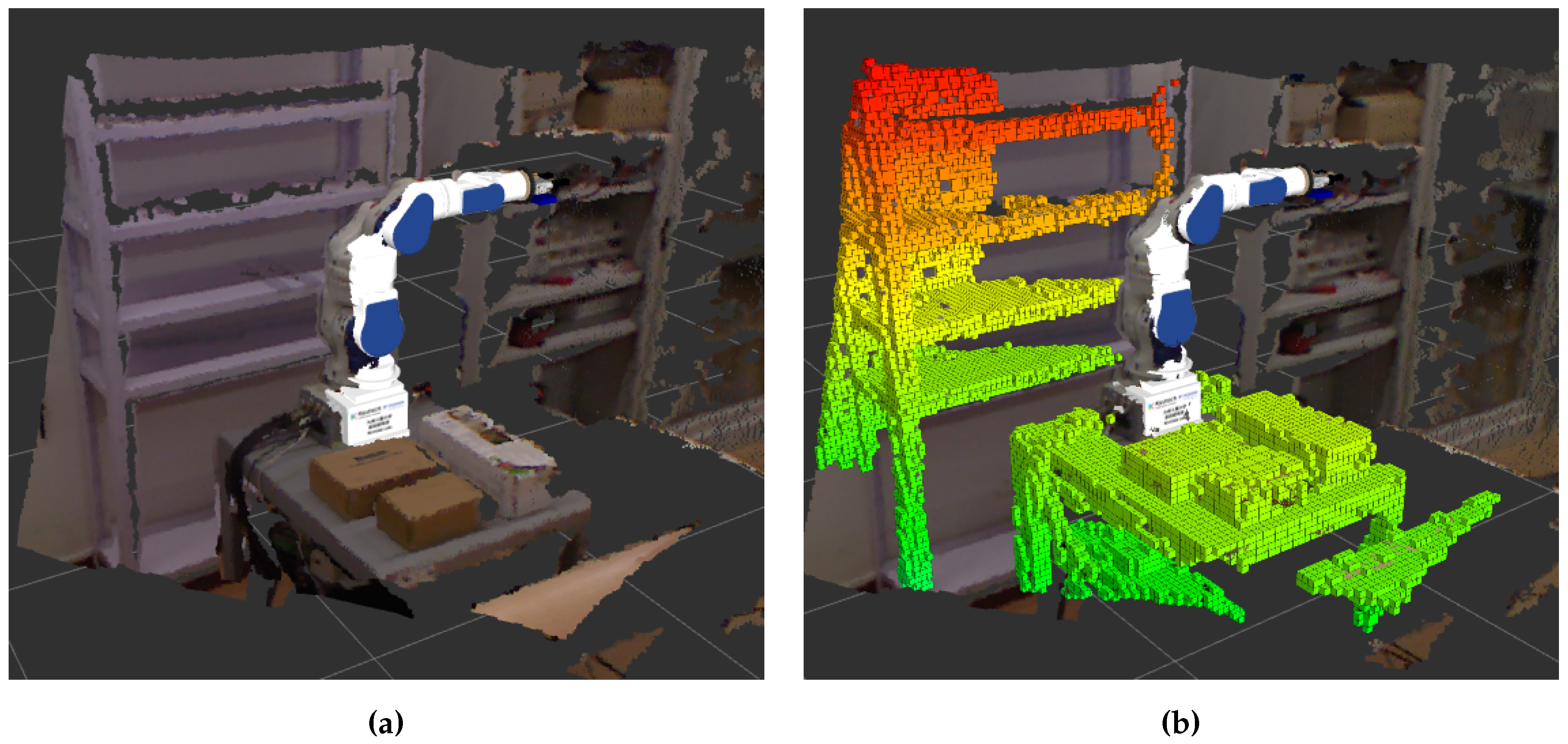
As seen in Figure 4, the PassThrough filter removes the points outside the interesting range. On the remaining point cloud, the estimation of the normal surface vectors is performed to determine the support plane. The clustering step closes the segmentation phase and provides data to the more specific description phase. The entire step-by-step segmentation process is illustrated in Figure 11.

The data preprocessing step uses an MLS filter and VoxelGrid filter to obtain an improved version of both the models and the cluster point clouds (see Figure 12).

The quality of the object recognition results is assessed through a manual check of the algorithm decisions: for each new scene, all the identified clusters are labeled, leading to the experimental data reported below.

Table 1. Mean values of OPRANSAC outputs: PC-models (Arabic numbers) and clusters (Roman numbers) as labeled in Figure 2a.

Target Object	Cluster
	I	II	III	IV	V	VI	VII
1	0.572	0.276	0.197	0.111	0	0	0
2	0.582	0.681	0.436	0.238	0.221	0	0.432
3	0.310	0.454	0.621	0.406	0.522	0.393	0.387
4	0.468	0.387	0.394	0.516	0.457	0.409	0.124
5	0.327	0.367	0.491	0.381	0.657	0.445	0.212
6	0	0	0	0	0	0.751	0
7	0	0.326	0.351	0.173	0.313	0	0.405

contains the average of the best fitness scores obtained by comparing each PC-model (row) with each cluster (column).

The objects with the most extensive surfaces (1 and 6) have a higher matching value with their respective clusters than the others. Consequently, the expected percentage of failure during recognition is low. In fact, their point cloud’s clusters have obviously more samples than those of the other objects and, therefore, their features will certainly have greater information content. On the opposite side, the clusters which represent the yellow glass (7) have fewer samples because of its small size. Moreover, the noise introduced through the sensor system makes very coarse and distorted clusters, which is why the feature’s precision and, therefore, the resulting fitness value are really compromised. The curvatures of the glass are not well defined in the clusters and that is why even the filtering techniques used are not enough to represent it better. So, the result is the low fitness value between the glass PC-model and the glass clusters. This result means that very often the glass PC-model can be confused with incorrect clusters, such as the small box (2) of similar height or the bottom part of the spray bottle (5) of similar geometry, as well as the coke bottle (3). The same difficulties could be encountered with object 4, because its geometry should be primarily defined by its handle, which should distinguish the corresponding cluster from the others. However, the detail may be unclear if the bottle is not frontally located or if it is too far from the camera.

Table 2. Summary of successes and failures based on 50 experimental tests: PC-models (Arabic numbers) and clusters (Roman numbers) as labeled in Figure 2a.

Target Object	Cluster
	I	II	III	IV	V	VI	VII
1	50	0	0	0	0	0	0
2	1	47	0	0	0	0	2
3	0	0	45	0	5	0	0
4	9	0	3	33	5	0	0
5	0	0	4	0	46	0	0
6	0	0	0	0	0	50	0
7	0	6	5	0	3	0	36

counts how many times the PC-model is recognized with the specific cluster, regardless of its fitness value. By aggregating the data, there are 307 true positive and 43 false positives, which corresponds to a correct recognition in the 87.71% of the cases and a wrong recognition in the remaining 12.29%. Generalizing these results, it is possible to construct a confusion matrix (

Table 3. Confusion matrix based on 50 experimental tests: PC-models (Arabic numbers) and clusters (Roman numbers) as labeled in Figure 2a.

Target Object	Cluster
	I	II	III	IV	V	VI	VII
1	1	0	0	0	0	0	0
2	0.02	0.94	0	0	0	0	0.04
3	0	0	0.90	0	0.1	0	0
4	0.18	0	0.06	0.66	0.1	0	0
5	0	0	0.08	0	0.92	0	0
6	0	0	0	0	0	1	0
7	0	0.12	0.10	0	0.06	0	0.72

), which indicates the quality of the algorithm and estimates its accuracy. Ideally, it should be an identity matrix, but due to false negatives of the tests, it is a bit deformed.

Finally, the ICP algorithm refines the initial coarse alignment provided by OPRANSAC. Figure 8 shows clear cases of convergence and the typical results.

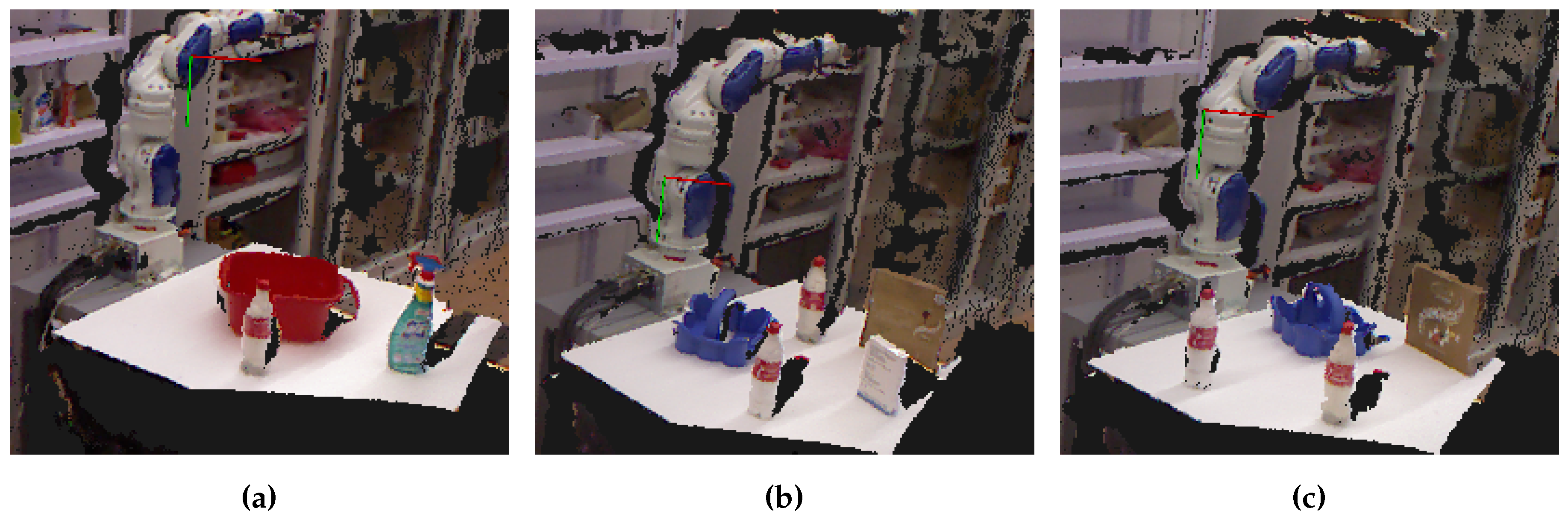
Robustness analysis. A further interesting test was performed to evaluate the algorithm robustness. Three limit cases were studied:

• scenarios with objects partially occluded, as in Figure 13a,c;
• scenarios with objects outside the data set, i.e., the purple container in Figure 13b,c;
• scenarios with more similar objects, e.g., two coke bottles as in Figure 13b,c.

Table 4. Fitness values of the experiment shown in Figure 13a: PC-models (Arabic numbers) and clusters (Roman numbers).

Target Object	Cluster
	III	V	VI
3	0.629	0.566	0.361
5	0.469	0.629	0.477
6	0	0	0.723

shows the matrix of the fitness values obtained at the end of the experiment in Figure 13a. By aligning a given PC-model (Arabic number labels) to the found clusters (Roman number labels), the computed fitness values underline how the partial occlusion of the red basin does not affect the performance of the algorithm.

Table 5. Fitness values of the experiment shown in Figure 13b: PC-models (Arabic numbers) and clusters (Roman numbers).

Target Object	Cluster
	I	II	IIIa	IIIb	Distraction
1	0.578	0.296	0	0	0
2	0.583	0.602	0.436	0.439	0.449
3	0.422	0.454	0.505	0.525	0.371

and

Table 6. Fitness values of the experiment shown in Figure 13c: PC-models (Arabic numbers) and clusters (Roman numbers).

Target Object	Cluster
	I	IIIa	IIIb	Distraction
1	0.478	0.382	0.312	0
3	0.418	0.583	0.558	0

, on the other hand, refer to the experiments in Figure 13b,c, respectively. In these scenarios, two difficulties are introduced: the purple container, which does not belong to the data set, and two similar coke bottles. The clustering process correctly produces two different clusters for the similar objects (labeled IIIa and IIIb in the table) and a cluster for the unknown object (labeled Distraction). Even in this case, the two bottles get the highest fitness values compared to the PC-model and, on the contrary, the cluster of the object outside the data set has the lowest fitness value.

Analysis of the execution time. Twenty experimental tests were done with the second data set (Figure 2b). In order to measure the execution time of the alignment step of the algorithm, the main parameters were set as in

Table 7. Alignment parameter settings.

OPRANSAC
ransac_max_iter	50,000
ransac_inlier_fraction	0.25
ransac_num_samples	3
ransac_similarity_thresh	0.9
ICP
icp_max_cor	0.01
icp_out_thresh	0.01
icp_max_iter	50,000

, and 20 scenes with 11 objects were prepared. The results, expressed in seconds, are reported in

Table 8. Execution times (in seconds).

	min	max	mean
OPRANSAC	31.25	134.7	75.7
ICP	0.5	1.4	0.7

. Note that the OPRANSAC step requires more computational time due to the introduction of the N-loop for each cluster. The refinement ICP phase shows a constant trend of around 700 ms, which is negligible.

Confusion matrix. Another interesting test was performed to deeply evaluate the algorithm robustness. The confusion matrix reported in

Table 9. Confusion matrix based on 20 observed scenes (recognition rate %): PC-models (capital letter) and clusters (lowercase letter) as labeled in Figure 2b. UR indicates unrecognition rates.

Target Object	Cluster
	a	b	c	d	e	f	g	h	i	j	k	UR
A	50	10	20	20	0	0	0	0	0	0	0	0
B	0	90	0	0	0	10	0	0	0	0	0	0
C	0	0	100	0	0	0	0	0	0	0	0	0
D	0	0	0	100	0	0	0	0	0	0	0	0
E	0	0	0	0	60	0	30	10	0	0	0	0
F	0	0	0	0	0	100	0	0	0	0	0	0
G	0	0	0	0	0	0	60	40	0	0	0	0
H	0	0	0	0	0	0	20	70	0	0	0	10
I	0	0	0	0	0	20	0	10	60	0	0	10
J	0	0	0	0	0	0	0	0	40	30	0	30
K	0	0	0	0	0	0	0	0	0	30	60	10

refers to the second data set. It is important to remark that without a criterion to exclude uncertain recognitions, objects are always recognized, and this can produce a high rate of false positives. A simple way to reduce this phenomenon is to fix a threshold, ${\delta }_{fit}$, to exclude the cases of poor likeness. This alternative method improves also the execution time of the algorithm because the expected loop can be interrupted if the average model–cluster correspondence is lower than ${\delta }_{fit}$. For each test, the algorithm is invoked, taking the PC-model of the object to be recognized as input. The algorithm output is a selected cluster with a fitness value, fitness. By comparing fitness with ${\delta }_{fit}$, it is possible to choose whether the correspondence is acceptable or not: if $fitness>{\delta }_{fit}$, the model–cluster association is valid (1); otherwise, no (0). By repeating this test for all object PC-models in the same scene and for 20 different scenarios, it is possible to report the percentage results in Table 9. The values in the last column represent the unrecognition rates ($fitness<{\delta }_{fit}$).

The C, D, and F boxes have a higher number of hits because their fitness match values are always the highest for their respective clusters than that with the other clusters, and so the percentage of failure, when the aim is to recognize these objects, is low. However, they are the objects with simpler geometry and larger surface extension, and this means that their point cloud clusters have obviously more samples than those of the others objects. On the other hand, the clusters of the G, H, I, and J objects have fewer points because they are small items and also their distance from the camera causes very coarse and distorted clusters. This limits the fitness values and therefore the success of the algorithm. The curvatures of the smaller objects are not well defined in the clusters, and even the filtering is not enough to represent them better. So, the result is a low fitness value implying that the desired target object is often confused with an incorrect cluster.

By aggregating the data, 220 tests were carried out: the algorithm produced 156 true positive and 52 false positives, which correspond to a correct recognition in 71% of the cases and a wrong recognition in 23%, while the remaining 6% of the considered cases did not produce any association at least equal to ${\delta }_{fit}$, i.e., unrecognized objects (UR).

3. Flexible Motion Planning

Perception of the workspace can drastically improve the flexibility of industrial systems. This section explains how to design a 3D vision system that can enable the robot to manipulate an object in a dynamic scene. The required accuracy must be sufficient to move the object into the space without causing damage, errors, and collisions. This work shows two independent strategies to achieve this goal. The first one, concerning the robot motion planning, is described in this section; the second one, concerning handling of the object itself, is described in Section 4. Motion planning while avoiding unnecessary robot reconfigurations and online collision avoidance with unexpected and uncertainly placed objects are the two main topics discussed below. The first problem was solved by integrating the Stochastic Trajectory Optimization for Motion Planning (STOMP) planner and the Trac-IK kinematics solver, developed by Traclabs [21], into the motion planning MoveIt! framework. The second problem was solved by developing a reactive control strategy based on distributed proximity sensors: an update of the planned trajectory is computed in real time to avoid collisions with unexpected objects in the scene.

3.1. Sensory System

Section 2.3.4 advises on the placement of the Intel RealSense camera for the optimality of the recognition and localization task. The suggested solution did not allow the RealSense to capture the whole robot workspace from the same camera. Thus, a second depth camera, a Microsoft Kinect, was integrated into the MoveIt! architecture. This sensor helps to faithfully reconstruct the 3D scene used for planning the robot motion.

The sensory system is completed with four proximity sensors mounted on the gripper (see Figure 19). This solution will better allow the robot to avoid collisions during the execution of trajectories. Objects which are not known or not perfectly captured through the camera are now detected. The proximity sensors were connected to the Arduino Mega 2560 microcontroller through a TinkerKit shield connected to the ROS (Robot Operating System) network via a serial interface.

3.2. Symmetric Grasp Planner

The first input data required by a motion planner in a pick and place task is the pose of the gripper required to grasp the object. In general, grasp planners are typically used to solve this problem, but, in this work, a simple parallel gripper was adopted. Therefore, grasp poses are manually pre-determined for each object. For each object model, two frames can be defined: the centroid frame and the grasping frame. For all objects without a particular symmetry (e.g., the spray bottle or the soap bottle), the grasping frame can be uniquely defined (e.g., on the model). However, grasping symmetric objects can require definition of the grasping frame only at run-time (e.g., on the aligned cluster). This crucial problem was investigated by considering common supermarket items.

Grasping frame for box-shaped items. Since $T_{ICP}^{camera}$ describes the pose of the chosen cluster with respect to the camera frame, the problem of defining the grasping frame can be difficult. Figure 14 clarifies this situation. The goal of the planner is to align the tool frame of the robot end effector to the grasping frame of the object (Figure 14a); then, not all the aligned cases are easy to reach. Due to the symmetry, an a priori fixed frame $T_{grasp}^{centroid}$ can bring the alignment algorithm to one of the four illustrated cases (Figure 14b–e). Situation (b) is the most favorable to the robot reach the grasping frame, but if the alignment algorithm generates case (e), then the end effector would collide with the support plane. Finally, the grasping poses in cases (c) and (d) are outside of the robot workspace. Therefore, heuristic criteria are hereafter introduced to define the grasping frame at run-time.

A possible solution separates the definition of the grasping point position from the definition of the object orientation. The origin of the grasping frame $p_{grasp}^{base}$ is the point which is both the closest to the origin of the robot base frame and the highest if compared to the plane surface. This solution guarantees that the grasp point is reached with as much ease as possible by the robot end effector.

The grasping orientation can be defined by assuming that the gripper approach axis is the x-axis and by taking the difference between $p_{grasp}^{base}$ and $p_{centroid}^{base}$. The unit vector of the x-axis of the grasping frame is set along the projection on the $(x,y)$ plane of the base frame of this difference, and the z-axis is aligned to the z-axis of the base frame and the y-axis to complete a right-handed frame.

Grasping frame for axisymmetric objects. In the case of axisymmetric objects, e.g., bottles, the selection of the grasping frame is simpler. A possible solution can be very similar to the previous one, with two main differences:

• for the position, there will be only two possible grasping points, as shown in Figure 15a,b;
• for the orientation, however, the choice is somewhat arbitrary, as shown in Figure 15c.

To be more specific, the grasping orientation can be fixed so that the robot grabs the object frontally with respect to itself (Figure 16a). However, if the cylinder position is too near the robot base, it is necessary to enlarge the inclination angle $\theta$ to allow the planner to find a feasible solution (see Figure 16b,c).

3.3. Motion Planning Pipeline

In everyday life, objects can be picked up, pushed, slid, and swept by humans hands. A remarkable set of strategies can be used to manipulate them, especially in complex scenes. On the other side, robots usually move objects simply through pick and place tasks.

IK constrained solution. During the experimental tests, it emerged that the default MoveIt! KDL kinematic solver, based on Newton’s method, had convergence problems due to the presence of joint limits. Thus, it was replaced with Trac-IK Solver. Its effectiveness is due to the merging of a simple extension to KDL’s Newton-based convergence algorithm with a Sequential Quadratic Programming (SQP) constrained nonlinear optimization approach. The first detects and mitigates local minima by random jumps; the second uses quasi-Newton methods that better handle joint limits.

By default, the IK search returns immediately when either of these algorithms converges to an answer. For this work, secondary constraints of manipulability are also provided in order to obtain the ‘best’ IK solution, which means to avoid unnecessary reconfigurations: virtual joint limits on relevant joints were used to compute the target configuration to keep it as close as possible to the starting configuration (see Section 5 for more details).

STOMP planner. Many planners were tested to compare the quality of the trajectories in detail. First, the default MoveIt! Open Motion Planning Library (OMPL) was tested. OMPL contains 11 motion planning algorithms which implement different SoA methods [22]. Fifty trials in five different scenarios were conducted for each planner to evaluate the success rate, as shown in Figure 17a. Only five motion planners provide at least 40% of the solutions in scenarios with obstacles.

OMPL provides consistent theoretical algorithms, but they are difficult to use in practice because a limited number of parameters can be tuned. This implies that the motion planning management is fully centralized in the algorithm itself and bonded by the user in a small part. The strong stochastic nature of sample-based motion planners gives unsatisfactory results because of often-unnatural planned trajectories, i.e., little regular curvature and no minimum distance from obstacles (see Figure 17b). For this reason, a special planner integration into the MoveIt! framework was used, i.e., the STOMP algorithm. It is a more recent optimal planning algorithm [22] that needs more computational time to answer, i.e., about 10 s compared with about 2 s needed by OMPL planners, but returns natural and smooth trajectories in scenarios with obstacles.

Obstacle avoidance. To plan collision-free motion, the sensory system captures the scene and sends its representation to the MoveIt! environment in the form of a point cloud (Figure 18a). The robot kinematic chain and everything described as a ’collidable’ object in the URDF (Unified Robot Description Format) file, which composes the RViz scene, is filtered. Finally, a 3D Occupancy Map (OctoMap) [23] is created to distinguish obstructing objects from the others, as shown in Figure 18b.

Flexible Collision Library (FCL) [24] is the default collision checking library of MoveIt!, and it supports OctoMap.

Task planning. The whole task follows the usual temporal segmentation, detailed in the previous version of this paper [1], in five phases: pre-grasp, grasp, manipulation, release, retreat. The output of the STOMP motion planner is a trajectory in the joint space made of a variable number of waypoints with a non-constant sampling frequency. The planner output cannot been used directly because the robot used for the tests (Figure 1) needs joint commands at a fixed rate of 50 Hz. Thus, an ROS node was developed to interpolate the planned waypoints at the desired rate with a fifth-order polynomial. This choice allows for maintaining velocity and acceleration continuity. The interpolated motion $q_d(t)$ can be finally used to move the robot in the joint space.

3.4. Reactive Motion Control

Even though STOMP plans a collision-free path by considering the current OctoMap, several uncertainties about the object poses or the possibility of partial views could lead to unexpected collisions. To counteract these issues, a real-time reactive control algorithm was developed. At execution time, it adapts the planned motion to the current scene. The method is based on the well-known artificial potential approach [25], further developed in [26], for a mobile manipulator. The planned motion in the joint space $q_d(t)$ is modified on the basis of the distances $d_i,i=1,\dots ,4$ computed by the four proximity sensors mounted on the gripper, as shown in Figure 19. A frame ${\Sigma }_i$ is attached to the ith sensor, with the orientation with respect to the robot base frame represented by the rotation matrix $R_{si}(q)$, where q is the current robot configuration.

The virtual repulsive force applied to the ith sensor is computed through a trigger with hysteresis:

$$s_{k+1}=\left\{\begin{array}{ll}1\hfill & \mathrm{if}{s}_k=0\mathrm{and}{d}_i<d_{mi}\hfill \\ 0\hfill & \mathrm{if}{s}_k=1\mathrm{and}{d}_i>d_{Mi}\hfill \\ s_k\hfill & \mathrm{otherwise}\hfill \end{array}\right.$$

(3)

$$f_i^{si}=\left\{\begin{array}{ll}{\left[\begin{array}{ccc}0& 0& -\alpha /d_i\end{array}\right]}^T\hfill & \mathrm{if}{s}_k=1\hfill \\ \begin{array}{ccc}0& 0& 0\end{array}{]}^T\hfill & \mathrm{if}{s}_k=0\hfill \end{array}\right.$$

(4)

where $\alpha$ is a suitable gain, $d_{mi}$ and $d_{Mi}$ are the two thresholds of the trigger, and $s_k$ is the trigger state at time k. When the trigger is not active, i.e., $s_k=0$, the reactive control is deactivated. The trigger is useful to avoid repeated switching when the distance is close to the minimum distance.

This repulsive force is then translated into a joint displacement as

$$\delta q=\beta {\displaystyle \sum _{i=1}^4}{J}_i^T(q)R_{si}{f}_i^{si},$$

(5)

where $J_i(q)$ is the arm Jacobian computed until the ith sensor frame, and $\beta$ is a gain (with the dimensions of a rotational compliance) translating the virtual elastic joint torque $J_i^T(q)R_{si}{f}_i^{si}$ into a joint displacement.

To avoid a joint jump when the trigger becomes active, $\delta q$ is smoothed through a low-pass filter.

This step endows the robot with the ability to react to scene uncertainties and dynamics as demonstrated by the experiment presented in Section 5.

4. Reactive Grasp Control

The pick and place task, typical of a supermarket scenario, requires manipulation of objects with different physical properties, like weight, friction, shape, and deformability. Moreover, the objects are subject to inertial forces due to the robot motion, which could be high depending on robot acceleration. Therefore, their manipulation based only on visual information might not be safe or robust, and object slipping events may be likely.

To enhance grasping safety and robustness, this study adopted a slipping control algorithm that adjusts the grasping force of the manipulated object in real time based on the tactile perception data provided by the sensorized fingers, described in [15,27]. The reactive grasp control algorithm was originally presented in [2], and it aims to avoid object slippage while applying the minimum required force so as to also safely manipulate deformable and fragile items.

The control algorithm used to generate the grasp force is here briefly described, but the interested reader can find more detail about the algorithm in [2].

The control strategy is model-based and exploits the Limit Surface (LS) theory [28]. Basically, the LS is an extension of the classical Coulomb friction model to the case of roto-translational motions. In such a case, the translational and the rotational dynamics are strictly coupled. This modeling is important if the object is not grasped at the Center of Gravity (CoG); in fact, in the case of torque loads, the appropriate grasp force to avoid slippage is usually much higher than that needed for balancing linear loads only.

The grasp force is computed as the sum of two contributions, i.e., $f_{n_s}$ and $f_{n_d}$,

$$f_n=f_{n_s}+f_{n_d}.$$

(6)

The first (static) contribution is computed based on the LS model based on the actual torsional and linear loads as measured by the sensorized fingers. The availability of this kind of measure allows the robot to safely pick objects of unknown weight and location at the CoG with respect to the grasping point, and this is an important feature for a robotic system that has to manipulate a large number of different objects, as in a retail store. However, this force is sufficient to avoid slippage only in quasi-static conditions, and thus, it might not be sufficient to guarantee a stable grasp, especially during the lifting phase, when the tangential force rapidly changes from zero to the weight of the object, or during the transporting phase, when inertial forces act on the object.

Therefore, there is a need for a second (dynamic) contribution, which is computed to counteract such uncertainties and external disturbances, based on the residual of a Kalman Filter (KF) fed with the tactile sensor measurements. The KF was designed according to a simplified dynamic model of the soft pad in contact with the manipulated object, and its residual is used as a signal able to detect pre-sliding conditions and thus to adjust the grasping force.

Figure 20a,b shows the results of the slipping avoidance algorithm during an experiment where the robot holds an object and an operator applies disturbances to the object. Such external loads are detected by the sensors as peaks in the tangential force (see Figure 20a), and the algorithm reacts by adjusting the grasp force so as to prevent slippage.

In the typical pick and place task, the reactive grasp controller is used to automatically calculate the grasp force during the lifting phase and during the motion of the robot, as will be described in Section 5.

5. Experimental Evaluation

Figure 1 shows the robot workspace in which the execution of a typical shelf refilling task was tested. A common supermarket scenario was simulated using some shelves and objects to grasp. As described in Section 2.2, the objects are randomly placed on a plane surface and their positions, their orientations, and their weight are not known. The goal of this experiment is to correctly grasp two objects (labeled F and K in Figure 2b) and place them on the shelf at a fixed target pose and very close to other objects. Every motion must avoid collisions with both the other objects of the scene and with other parts of the robot environment that the sensor system roughly localizes, hence the need for actual distance information from the proximity sensors used at execution time to locally adjust the planned trajectory.

Object recognition and localization. The software developed in this work saved an instantaneous picture of the current scene by capturing the depth image through the RealSense camera. The data are then converted in the form of a point cloud. This file becomes the input of the hybrid pipeline in order to recognize a specific object, whose PC-model is properly specified. The algorithm provides the object pose with respect to the robot base represented by the $T_{grasp}^{base}$ homogeneous transformation matrix.

Offline trajectory planning. The $T_{grasp}^{base}$ matrix indicates to the motion planner the picking pose that the robot end effector must reach. The planning pipeline described in [1] is sequentially executed. The STOMP planner is invoked at every step: the robot current configuration allows the Trac-IK solver to provide a robot collision-free target configuration. Then, STOMP plans the correct collision-free trajectory by exploiting FCL. To avoid unnatural reconfigurations, during the experimental tests, some critical joint limits were identified: S, E, and T joints (see Figure 1) proved to be the cause of the robot reconfigurations. Two sets of virtual joint limits were defined for the selected joint angles: one with positive ranges and the other with negative ones. The IK solver chooses between the two sets according to the signs of the selected joints in the robot current configuration, thus trying to avoid a reconfiguration, e.g., from elbow up to elbow down.

Reactive grasp control. In the lifting phase, and during the whole motion, the grasp force is computed by the slipping avoidance algorithm. Figure 21 shows the lifting phase. Notice as the forces are initially zero and suddenly rise, in particular, the tangential force $f_t$ rises as the object is lifted. The grasp force automatically grows, but notice that it rises very quickly and it has a peak due to the dynamic force contribution illustrated in Section 4. This reaction is sufficient to counteract the inertial forces that build up in the lifting phase, hence avoiding object slipping.

Reactive motion control. In order to test the benefits of the reactive motion control, some objects are placed on the shelving unit on purpose and the robot is asked to place the grasped object in a position very close to them. The result is that the proximity sensors locally correct the STOMP planned trajectory. In this task, the proximity sensor thresholds in (4) are set as follows:

• $d_{m_i}$ = 50 mm, $d_{M_i}$ = 100 mm, i = 1, 2, 4
• $d_{m_3}$ = 70 mm, $d_{M_3}$ = 170 mm

while the gains are $\alpha$ = 5 Nmm and $\beta$ = 0.3 rad/Nm. Specifically, the use of proximity sensors is fundamental during the place phase. As shown in Figure 22a and in the distance signals reported in Figure 22b, when the robot end effector enters the shelving unit, the third proximity sensor (with reference to the numbers in Figure 19) detects the upper edge of the shelf, which produces a repulsive downward force applied to the end effector computed as in (4). This force provides a joint displacement $\delta q$ which is added to the planned configuration $q_d(t)$ until the specific sensor reads distances into the reactive range. Figure 23 reports some planned and actual joint positions. Then, the second sensor detects the presence of an obstacle, which produces a repulsive rightward force applied to the end effector. From this moment on, the joint displacement $\delta q$ overlaps the effects of both sensors. Subsequently, the end effector tries to reach the deep target pose following the modified planned trajectory. Thus, even the right object is detected by the first sensor. A new repulsive force is generated and the combination of the other two produces a new displacement. In this way, the grasped object is safely placed on the shelf. A video of the complete experiment can be found at the following link: https://www.researchgate.net/publication/328881061_REFILLS_project_video.

Even though the recognition algorithm was tested on all the labeled objects of the data sets (Section 2.3.4), the experimental evaluation of the whole task was carried out on a subset of them (E, F, I, and K). The choice of the subset is due to the physical limit of the gripper that can grasp only objects with a width less than 55 mm.

Table 10. Recognition and localization success rate based on 20 observed scenes.

Target Object	Rate %
	Success	Not Recognized	Not Localized
E	55	40	5
F	100	0	0
I	60	40	0
K	50	40	10

summarizes the success rate of the recognition and localization task obtained by analyzing 20 experimental tests. The task is considered successful if the object is correctly recognized and if the localization accuracy is high enough to allow proper grasping of the object. The unsuccessful executions caused by an incorrect recognition (‘Not recognized’ column) are more frequent than errors caused only by localization (‘Not localized’ column). This is due to the inclusion of the localization step in the recognition step. The most frequent errors are related to object K, which has a diameter of about 50 mm that results into a tight grasp tolerance.

Some of the software modules exploited to perform the experiment were taken from existing software libraries and used as they are. Other modules were developed purposefully for this research work, and the rest are a result of the integration of existing modules into more complex frameworks. To highlight the actual contribution of the paper,

Table 11. Recap of relevant software modules which were developed and integrated into the proposed system. Empty entries in the 4th column mean that the corresponding software modules were used as they are.

Research Topic	Software Package	Software Modules	Integrated Software Modules	Developed Software Modules
Object Recognition and Localization	PCL	Filters
		Segmentation
		Feature Extraction
		Correspondences	Hybrid Pipeline	OPRANSAC
		Alignment
Motion Planning	MoveIt!	IK	Trac-IK
		Planner	STOMP
		Collision Check
	Grasp Planner			Symmetric Grasp Planner
Reactive Control	REFILLS software package	Robot control at arm level		Proximity based slipping avoidance
		Robot control at gripper level		Limit Surface slipping avoidance

explicitly reports the list of the modules belonging to these three categories.

6. Conclusions

This work reports an experimental study of different methods for the planning and control of a robot performing a complete fetch and carry task typical of the in-store logistics scenario, where a number of different items have been handled. The considered methods range from object recognition and localization in cluttered scenes to the motion planning and reactive control used to improve the success rate of the task. Novel elements are proposed in all of the technologies that were revealed to be essential for the successful execution of the task in a real setting. Limitations to the approach are mainly due to the perception system and the computational time for object recognition. The objects are required to be placed at a certain distance from each other, and no transparent or thin or polished objects can be handled, as it is difficult to reconstruct a good quality point cloud in such cases. Future work will be devoted to integrating other depth cameras to better cover the scene or combining sensors (e.g., tactile sensors [29]), as well as evaluating the system performances by using a larger object data set. A parallel implementation of the OPRANSAC algorithm could be developed to decrease the computational time of the object recognition step. The proposed approach could be extended by using a grasp planner to apply the strategy to a larger variety of object shapes.

References

1. Costanzo, M.; De Maria, G.; Lettera, G.; Natale, C.; Pirozzi, S. Flexible Motion Planning for Object Manipulation in Cluttered Scenes. In Proceedings of the 15th International Conference on Informatics in Control, Automation and Robotic—Volume 2: ICINCO, INSTICC, Porto, Portugal, 29–31 July 2018; SciTePress: Porto, Portugal, 2018; pp. 110–121. [Google Scholar]
2. Costanzo, M.; De Maria, G.; Natale, C. Slipping Control Algorithms for Object Manipulation with Sensorized Parallel Grippers. In Proceedings of the 2018 IEEE International Conference on Robotics and Automation, Brisbane, Australia, 21–25 May 2018. [Google Scholar]
3. Kuffner, J.; LaValle, S. RRT-connect: An efficient approach to single-query path planning. In Proceedings of the Millennium Conference, IEEE International Conference on Robotics and Automation, Proceedings 2000 ICRA, San Francisco, CA, USA, 24–28 April 2000; Symposia Proceedings (Cat. No.00CH37065). pp. 995–1001. [Google Scholar]
4. Kavraki, L.; Svestka, P.; Latombe, J.C.; Overmars, M. Probabilistic roadmaps for path planning in high-dimensional configuration spaces. IEEE Trans. Robot. Autom. 1996, 12, 566–580. [Google Scholar] [CrossRef] [Green Version]
5. Phillips, J.M.; Bedrosian, N.; Kavraki, L. Guided Expansive Spaces Trees: A Search Strategy for Motion- and Cost-Constrained State Spaces. In Proceedings of the 2004 IEEE International Conference on Robotics and Automation, New Orleans, LA, USA, 26 April–1 May 2004; pp. 3968–3973. [Google Scholar]
6. Şucan, I.A.; Kavraki, L.E. Kinodynamic Motion Planning by Interior-Exterior Cell Exploration. In Springer Tracts in Advanced Robotics; Springer: Berlin/Heidelberg, Germany, 2009; pp. 449–464. [Google Scholar]
7. Khokar, K.; Beeson, P.; Burridge, R. Implementation of KDL Inverse Kinematics Routine on the Atlas Humanoid Robot. Procedia Comput. Sci. 2015, 46, 1441–1448. [Google Scholar] [CrossRef]
8. Rusu, R.B.; Blodow, N.; Beetz, M. Fast Point Feature Histograms (FPFH) for 3D registration. In Proceedings of the 2009 IEEE International Conference on Robotics and Automation, Kobe, Japan, 12–17 May 2009; pp. 3212–3217. [Google Scholar]
9. Tombari, F.; Salti, S.; Stefano, L.D. Unique Signatures of Histograms for Local Surface Description. In Lecture Notes in Computer Science, Proceeding of the Computer Vision—ECCV 2010, Crete, Greece, 5–11 September 2010; Springer: Berlin/Heidelberg, Germany, 2010; pp. 356–369. [Google Scholar]
10. Rusu, R.B.; Bradski, G.; Thibaux, R.; Hsu, J. Fast 3D recognition and pose using the Viewpoint Feature Histogram. In Proceedings of the 2010 IEEE/RSJ International Conference on Intelligent Robots and Systems, Taipei, Taiwan, 18–22 October 2010; pp. 1–4. [Google Scholar]
11. Rusu, R.B.; Cousins, S. 3D is Here: Point Cloud Library (PCL). In Proceedings of the 2011 IEEE International Conference on Robotics and Automation, Shanghai, China, 9–13 May 2011. [Google Scholar]
12. Aldoma, A.; Marton, Z.C.; Tombari, F.; Wohlkinger, W.; Potthast, C.; Zeisl, B.; Rusu, R.; Gedikli, S.; Vincze, M. Tutorial: Point Cloud Library: Three-Dimensional Object Recognition and 6 DOF Pose Estimation. IEEE Robot. Autom. Mag. 2012, 19, 80–91. [Google Scholar] [CrossRef]
13. Papazov, C.; Burschka, D. An Efficient RANSAC for 3D Object Recognition in Noisy and Occluded Scenes. In Lecture Notes in Computer Science, Proceeding of the Computer Vision—ECCV 2010, Crete, Greece, 5–11 September 2010; Springer: Berlin/Heidelberg, Germany, 2011; pp. 135–148. [Google Scholar]
14. Aldoma, A.; Vincze, M.; Blodow, N.; Gossow, D.; Gedikli, S.; Rusu, R.B.; Bradski, G. CAD-model recognition and 6DOF pose estimation using 3D cues. In Proceedings of the 2011 IEEE International Conference on Computer Vision Workshops (ICCV Workshops), Barcelona, Spain, 6–13 November 2011; pp. 585–592. [Google Scholar]
15. De Maria, G.; Natale, C.; Pirozzi, S. Force/tactile sensor for robotic applications. Sens. Actuators A Phys. 2012, 175, 60–72. [Google Scholar] [CrossRef]
16. Nakhaeinia, D.; Payeur, P.; Laganiére, R. A Mode-Switching Motion Control System for Reactive Interaction and Surface Following Using Industrial Robots. IEEE/CAA J. Autom. Sin. 2018, 5, 670–682. [Google Scholar] [CrossRef]
17. Kopf, C.; Heindl, C.; Ankerl, M.; Bauer, H.; Pichler, A. ReconstructMe—Towards a Full Autonomous Bust Generator. In Proceedings of the 5th International Conference on 3D Body Scanning Technologies, Lugano, Switzerland, 21–22 October 2014; pp. 184–190. [Google Scholar]
18. Rusinkiewicz, S.; Levoy, M. Efficient variants of the ICP algorithm. In Proceedings of the IEEE Third International Conference on 3-D Digital Imaging and Modeling, Quebec City, QC, Canada, 28 May–1 June 2001; pp. 145–152. [Google Scholar] [Green Version]
19. Buch, A.G.; Kraft, D.; Kamarainen, J.K.; Petersen, H.G.; Kruger, N. Pose estimation using local structure-specific shape and appearance context. In Proceedings of the 2013 IEEE International Conference on Robotics and Automation, Karlsruhe, Germany, 6–10 May 2013; pp. 2080–2087. [Google Scholar]
20. Steder, B.; Rusu, R.B.; Konolige, K.; Burgard, W. Point feature extraction on 3D range scans taking into account object boundaries. In Proceedings of the 2011 IEEE International Conference on Robotics and Automation, Shanghai, China, 9–13 May 2011. [Google Scholar]
21. Beeson, P.; Ames, B. TRAC-IK: An open-source library for improved solving of generic inverse kinematics. In Proceedings of the 2015 IEEE-RAS 15th International Conference on Humanoid Robots (Humanoids), Seoul, Korea, 3–5 November 2015; pp. 928–935. [Google Scholar]
22. Kalakrishnan, M.; Chitta, S.; Theodorou, E.; Pastor, P.; Schaal, S. STOMP: Stochastic trajectory optimization for motion planning. In Proceedings of the 2011 IEEE International Conference on Robotics and Automation, Shanghai, China, 9–13 May 2011; pp. 4569–4574. [Google Scholar]
23. Hornung, A.; Wurm, K.M.; Bennewitz, M.; Stachniss, C.; Burgard, W. OctoMap: An Efficient Probabilistic 3D Mapping Framework Based on Octrees. Auton. Rob. 2013, 34, 189–206. [Google Scholar] [CrossRef]
24. Pan, J.; Chitta, S.; Manocha, D. FCL: A general purpose library for collision and proximity queries. In Proceedings of the 2012 IEEE International Conference on Robotics and Automation, St. Paul, MN, USA, 14–18 May 2012; pp. 3859–3866. [Google Scholar]
25. Khatib, O. Real-time obstacle avoidance for manipulators and mobile robots. Int. J. Rob. Res. 1986, 5, 90–98. [Google Scholar] [CrossRef]
26. Falco, P.; Natale, C. Low-level flexible planning for mobile manipulators: A distributed perception approach. Adv. Robot. 2014, 28, 1431–1444. [Google Scholar] [CrossRef]
27. Cirillo, A.; Cirillo, P.; De Maria, G.; Natale, C.; Pirozzi, S. Control of linear and rotational slippage based on six-axis force/tactile sensor. In Proceedings of the 2017 IEEE International Conference on Robotics and Automation (ICRA), Singapore, 29 May–3 June 2017; pp. 1587–1594. [Google Scholar]
28. Howe, R.D.; Cutkosky, M.R. Practical Force-Motion Models for Sliding Manipulation. Int. J. Robot. Res. 1996, 15, 557–572. [Google Scholar] [CrossRef]
29. Falco, P.; Lu, S.; Cirillo, A.; Natale, C.; Pirozzi, S.; Lee, D. Cross-modal visuo-tactile object recognition using robotic active exploration. In Proceedings of the 2017 IEEE International Conference on Robotics and Automation (ICRA), Singapore, 29 May–3 June 2017; pp. 5273–5280. [Google Scholar]
Figure 1. Experimental setup.
Robotics 07 00076 g001
Figure 2. (a) Initial object training set. (b) Final object training set.
Robotics 07 00076 g002
Figure 3. Some objects of the data set (top) and their reconstructed 3D CAD-models (bottom).
Robotics 07 00076 g003
Figure 4. The state-of-the art (SoA) local and global pipeline and their combination into the proposed hybrid pipeline.
Robotics 07 00076 g004
Figure 5. k dependence for the plane segmentation. From left to right: k = 5 ; k = 50 ; k = 100 .
Robotics 07 00076 g005
Figure 6. Outcome of the clustering process.
Robotics 07 00076 g006
Figure 7. Fast Point Feature Histograms (FPFH) descriptors of two objects in the set: clusters (white) and point cloud (PC)-model (green).
Robotics 07 00076 g007
Figure 8. Alignment phase: (yellow) Iterative Closest Point (ICP) adjusts the (blue) Optimized RANdom SAmple Consensus (OPRANSAC) coarse alignment on the (green) cluster.
Robotics 07 00076 g008
Figure 9. Classification of points near the edges of a box: object edges (yellow), veil points (red), and shadow edges (light blue).
Robotics 07 00076 g009
Figure 10. Key-point extraction from the observed scene: failure of the correspondences (red) of the PC-model (yellow) on the whole scene.
Robotics 07 00076 g010
Figure 11. The segmentation process. Following the arrows: the observed scene is acquired; the PassThrough filter is applied and the normal vectors are estimated; the support plane is removed; finally, the clustering process is executed.
Robotics 07 00076 g011
Figure 12. From left to right: CAD-models, PC-models, Moving Least Square (MLS) filter applied to PC-models, final VoxelGrid downsampling.
Robotics 07 00076 g012
Figure 13. Sample scenes to test the robustness of the algorithm: (a) Scenario with partial occlusion; (b) scenario with an object outside the data set and similar objects; (c) scenario with partial occlusion, an object outside the data set and similar objects.
Robotics 07 00076 g013
Figure 14. Critical cases in the definition of the grasping frame for parallelepiped objects: (a) Alignment of the robot tool frame to the object grasping frame; (b) the grasping frame is reachable and collision-free; (c,d) the grasping frame is outside the robot workspace; (e) the grasping frame is reachable but in collision with the support plane.
Robotics 07 00076 g014
Figure 15. Critical cases in the definition of the grasping frame for axisymmetric objects: (a) The grasping frame is reachable and collision-free; (b) the grasping frame is outside the robot workspace and in collision with the support plane; (c) arbitrary choice of the grasping frame orientation of x and y axes.
Robotics 07 00076 g015
Figure 16. Definition of the grasping frame orientation of x and y axes for axisymmetric objects: (a) Frontal grasp; (b) admissible area for lateral grasp; (c) feasible example of lateral grasp.
Robotics 07 00076 g016
Figure 17. (a) Fifty-trial success rate of standard motion planners in five different scenarios. (b) Typical Open Motion Planning Library (OMPL) planned path vs Stochastic Trajectory Optimization for Motion Planning (STOMP) solution.
Robotics 07 00076 g017
Figure 18. (a) Point cloud into Robot Operating System (ROS) environment; (b) 3D Occupancy Map (OctoMap).
Robotics 07 00076 g018
Figure 19. Gripper with proximity sensors (red arrows are the z-axes of the sensor frames).
Robotics 07 00076 g019
Figure 20. Validation experiment for the slipping avoidance algorithm. (a) Force and torque measured by the tactile/force sensor: grasp force in blue, tangential force ( f t ) in red, torsional moment ( τ z ) in yellow. (b) Disturbances applied by an operator.
Robotics 07 00076 g020
Figure 21. Force and torque measured by the sensorized fingers during the lifting subtask: grasp force in blue, tangential force ( f t ) in red, torsional moment ( τ z ) in yellow.
Robotics 07 00076 g021
Figure 22. (a) Example of a place subtask. (b) Distances measured by the four proximity sensors during the place subtask (blue) and thresholds values of Equation (3) (red).
Robotics 07 00076 g022
Figure 23. Planned (blue) and actual (red) positions of the first three arm joints.
Robotics 07 00076 g023