Collision Avoidance with Deep Learning in a Digital Twin for Industrial Collaborative Robot Manipulation

Abstract

Safe human–robot collaboration remains a critical challenge in manufacturing. Traditional safety approaches, such as cages and proximity sensors, are often insufficient for dynamic human interaction. This paper presents a digital twin-based collision avoidance framework for industrial collaborative robot manipulation. The system integrates RGB-D sensing, human pose estimation using Ultralytics YOLO26s-pose, Kalman-filter-based 3D arm tracking, short-term motion prediction, and QP-based reactive motion control. Human arm keypoints detected from RGB-D images are reconstructed in 3D, transformed into the robot base frame, and tracked during temporary occlusion using Kalman filtering with kinematic constraints. Predicted human–robot clearance is evaluated to trigger speed reduction, stopping, or collision avoidance commands. The framework was implemented with a UR10e robot, an Intel RealSense D435 camera, a Unity3D digital twin, and ROS communication. Controlled laboratory experiments demonstrated the proof-of-concept feasibility of the integrated framework for tracking human arm motion, anticipating proximity risk, and triggering protective robot responses. The results do not establish deployment readiness in complex industrial or multi-participant environments.

1. Introduction

Representations and models of humans play a crucial role in the development and implementation of systems ranging from robotic motion planning [1] to Industry 5 [2]. Despite the growing adoption of collaborative robots (cobots), companies continue to experience workplace and industrial accidents [3], highlighting the need for improved safety mechanisms.

The ever-increasing integration of robots into manufacturing has accelerated the demand for reliable human–robot interaction safety systems [4]. Traditional methods relying on physical barriers or basic proximity sensors often limit flexibility and reconfigurability and hinder close interaction [5]. Digital twin (DT) technology introduces a potential alternative by enabling a real-time virtual model of physical systems that can simulate and monitor operational states [2,6].

At the same time, advances in deep learning-based computer vision, particularly human pose estimation, have significantly improved human recognition and scene understanding [7,8]. Integrating pose estimation with a digital twin enables a more adaptive safety framework in which human motion can inform protective robot responses.

Although digital twins have been widely used for robot visualization, state monitoring, predictive maintenance, and process optimization, their use in safety-critical human–robot collaboration remains limited. In particular, monitoring-oriented systems do not necessarily address three practical problems: temporary loss or inconsistency of RGB-D human pose measurements, delayed intervention when safety decisions rely only on current separation, and the conversion of perceived risk into physically feasible robot commands. This study does not claim novelty for YOLO26s-pose estimation, Kalman filtering, digital twin modeling, or QP control individually. Instead, its contribution lies in coupling these components through a closed-loop perception–prediction–control architecture. The framework maintains bounded human arm estimates during temporary measurement loss, predicts future capsule-based human–robot clearance, and translates the resulting risk into constrained speed reduction, stopping, or collision avoidance commands synchronized between the digital twin and the physical robot. The main contributions of this work are as follows: because the perception, estimation, prediction, and control stages are tightly coupled, the experiments compare integrated configurations and do not quantify the independent contribution of every individual module.

• A closed-loop DT-based safety architecture is developed that connects RGB-D human perception, short-term risk prediction, and constrained robot control, extending the DT from passive visualization and monitoring to active safety intervention.
• A robust 3D human arm tracking pipeline is implemented by combining depth validity checking, eye-to-hand transformation, bounded Kalman prediction, kinematic constraints, and covariance-based safety margin adjustment. The pipeline maintains usable arm-state estimates during temporary measurement loss while preventing uncertain long-term extrapolation; its evaluation is system-level and does not isolate the Kalman filter or kinematic constraints independently.
• A short-term capsule-based clearance prediction method is implemented to identify impending reductions in human–robot separation before they are fully reflected in the current-distance measurement. Its incremental effect is evaluated against a no-prediction configuration and a zero-order-hold reference; no claim of superiority over other prediction methods is made.
• A QP/NEO-based controller converts current and predicted safety risk into physically feasible joint-velocity commands while enforcing obstacle avoidance, joint limit, and self-collision constraints. Same-sequence comparisons of the integrated configurations show greater tracking availability, smoother reconstructed arm motion, less stopped time, and a higher mean-operating-speed command under the tested laboratory conditions.

The remainder of this paper is organized as follows. Section 2 reviews related studies on human pose estimation, digital twins, and collision avoidance in human–robot collaboration. Section 3 describes the proposed system architecture, eye-to-hand calibration, human arm skeleton estimation, short-term motion prediction, clearance computation, and reactive motion control algorithm. Section 4 presents the experimental setup and discusses the calibration accuracy, Kalman-based occlusion recovery, predictive safety response, digital twin visualization, and real-robot collision avoidance results. Section 5 concludes this paper and outlines future research directions.

2. Related Work

This section highlights prior studies on human pose estimation and digital twin technologies in human–robot collaboration.

2.1. Human Pose Estimation

Several studies have investigated learning-based collision avoidance methods for autonomous and robotic systems. Refs. [9,10] examined collision prediction and response, whereas refs. [11,12] used deep learning or reinforcement learning to improve robotic safety and navigation. These studies primarily addressed sensing, motion planning, or control without integrating pose estimation into a closed-loop digital twin framework.

Pose estimation using convolutional neural networks, such as OpenPose [7] and MediaPipe [13], provides an effective means of capturing human body keypoints. These models have been applied to gesture recognition [7], but few studies have integrated them with robotic DTs for real-time safety intervention [2].

2.2. Digital Twin in Human–Robot Collaboration

Human–robot collaboration has traditionally depended on mechanical safety measures and limited perception systems. Early frameworks relied on fixed safety zones and light curtains [14], which restricted task adaptability. With the emergence of collaborative robots (cobots), vision-based systems have gained importance in ensuring dynamic safety [15].

Liao et al. [16] presented an improved moving-target-tracking algorithm based on the YOLO model for detection. The experimental results showed that the algorithm achieved high multi-target-tracking accuracy and stability in complex industrial environments, providing a valuable reference for future research. However, the study did not include the presence or involvement of humans in the research framework.

Lian et al. [17] proposed a digital twin-based security-monitoring method for production lines by integrating physical and virtual models, synchronized twin data, and a service platform for real-time monitoring. In that work, twin data represented bidirectional information exchange between the production line and its digital representation, including sensor measurements, actuator states, and process variables. However, human involvement in the framework was limited.

In summary, DTs have increasingly been adopted in industrial robotics for predictive maintenance, process optimization, and remote monitoring [2,18,19]. However, integrating deep learning-based perception into DTs for safety-critical decision making remains limited [4]. The proposed approach contributes to the effort to address this gap by coupling a DT model of a robot arm with live human pose estimation for collision prevention.

3. Methods

This section presents the system overview, the eye-to-hand calibration method for aligning the camera and robot frames, and the optimization algorithm used for reactive motion control of the manipulator.

3.1. System Overview

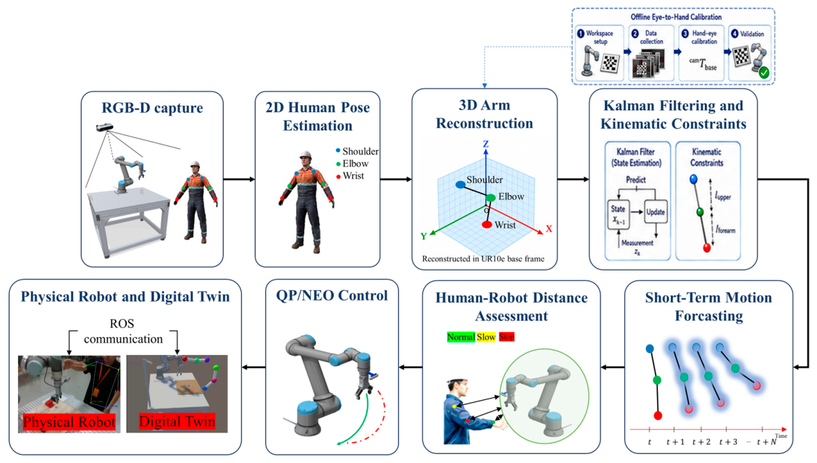
The proposed system follows an integrated perception–prediction–control workflow for real-time human–robot collision avoidance, as shown in Figure 1. First, RGB-D sensing acquires color and depth frames to monitor the shared human–robot workspace. The Ultralytics YOLO26s-pose model (checkpoint: yolo26s-pose.pt), documented by Jocher et al. [20] and independently analyzed by Sapkota et al. [21], then estimates 2D human arm keypoints and infers the hand position. These keypoints are reconstructed into 3D coordinates using depth information and transformed into the robot base frame. To improve robustness against noisy observations and temporary occlusion, Kalman filtering and kinematic constraints are applied to estimate continuous human arm states. The filtered arm states are further used for short-term motion forecasting to predict future human–robot distances. Current and predicted distances between the human arm and robot links are continuously assessed. Based on this assessment, the safety decision and reactive motion control (QP/NEO) module adjusts the robot motion by reducing joint velocity, enforcing obstacle avoidance, joint limits, and self-collision constraints. Finally, the physical robot and digital twin are synchronized through ROS, allowing the safety response and robot state to be updated in both the real and virtual environments.

3.2. Eye-to-Hand Calibration

The eye-to-hand calibration process establishes the rigid spatial transformation between a fixed camera and the robot coordinate system. This relationship enables the robot to interpret visual information in its own reference frame, which is a prerequisite for vision-guided manipulation and autonomous perception. Unlike an eye-in-hand configuration, in which the camera moves with the manipulator, the eye-to-hand configuration uses a stationary camera to observe the robot workspace.

The transformation between the robot base and the camera coordinate system is defined as a homogeneous transformation matrix:

$$X=[R\mid t]$$

(1)

where $R\in SO\left(3\right)$ denotes the rotation matrix, and $t\in {\mathbb{R}}^3$ represents the translation vector. Given multiple robot poses and corresponding observations of a calibration target, the calibration problem can be expressed as

$$A_{i}X=X{B}_i, i=1,2,\dots ,n$$

(2)

where

• $A_i$ is the transformation from the robot base to the end-effector for pose $i$, obtained from the robot’s kinematic model.
• $B_i$ is the transformation from the calibration target to the camera coordinate system for the same pose, computed from image-based pose estimation.

The objective is to estimate $X$, the homogeneous transformation from the camera frame to the robot-base frame. In the remainder of this paper, this calibrated transform is written as ${}^B\mathrm{T}_C$. The equation is solved using least-squares optimization over multiple observations to minimize rotational and translational residuals.

The calibration experiment was conducted using a fixed RGB camera positioned to observe the robot’s entire workspace. A checkerboard target of known geometry was mounted on the robot end-effector. The robot was commanded to move to multiple poses (15 in total), covering a broad range of orientations and positions within the camera’s field of view. For each pose, the following data were recorded:

• The end-effector pose with respect to the robot base frame, obtained from the robot controller.
• The target pose with respect to the camera, estimated from the detected checkerboard corners.

The calibration data pairs $(A_i,B_i)$ were processed using the Tsai–Lenz algorithm [22] to determine the transformation matrix between the robot base and the camera coordinate system. This algorithm separately estimates the rotational and translational components of the transformation and then combines them into a single homogeneous transformation matrix:

$$X=\left[\begin{array}{cc}R& t\\ 0& 1\end{array}\right]$$

(3)

where $R$ and $t$ denote the rotation and translation components, respectively. To improve robustness, outlier poses were removed based on the reprojection error threshold computed from the camera observations.

To evaluate the calibration accuracy, the estimated transformation matrix $X$ was used to project known 3D target points from the robot base frame into the image plane. The reprojection error between the observed and projected points was computed as

$$e={\displaystyle \frac{1}{N}}{\displaystyle {\sum }_{i=1}^N}\parallel p_i^{\mathrm{obs}}-p_i^{\mathrm{proj}}\parallel$$

(4)

where $p_i^{\mathrm{obs}}$ and $p_i^{\mathrm{proj}}$ are the observed and projected pixel coordinates, respectively. A smaller reprojection error indicates better alignment between the robot and camera coordinate systems, reflecting higher calibration accuracy.

3.3. Human Arm Skeleton Estimation

3.3.1. RGB-D-Based Human Arm Reconstruction

Let $\mathrm{a}\in \left\{L,R\right\}$ denote the left and right arms, and let $j\in \left\{s,e,w,h\right\}$ denote the shoulder, elbow, wrist, and hand respectively. At frame $k$, YOLO26s-pose inference gives a 2D keypoint measurement:

$$u_{a,j,k}={\left[\begin{array}{ccc}{u}_{a,j,k}& v_{a,j,k}& c_{a,j,k}\end{array}\right]}^T,$$

(5)

where $u_{a,j,k}$ and $v_{a,j,k}$ are pixel coordinates, and $c_{a,j,k}$ is the keypoint confidence.

The aligned depth image provides the depth value $Z_{a,j,k}$. To suppress local depth noise, $Z_{a,j,k}$ is computed as the median valid depth in a local window around the keypoint.

$${\mathrm{p}}_{a,j,k}^C=Z_{a,j,k}\left[\begin{array}{c}\left(u_{a,j,k}-c_x\right)/f_x\\ \left(v_{a,j,k}-c_y\right)/f_y\\ 1\end{array}\right],$$

(6)

Here, $f_x$, $f_y$, $c_x$, and $c_y$ are the intrinsic parameters of the RealSense D435 camera.

The 3D point is transformed from the camera frame C to the robot-base frame B using the calibrated homogeneous transformation ${}^B\mathrm{T}_C$:

$$\left[\begin{array}{c}{\mathrm{p}}_{a,j,k}^B\\ 1\end{array}\right]={}^B\mathrm{T}_C\left[\begin{array}{c}{\mathrm{p}}_{a,j,k}^C\\ 1\end{array}\right].$$

(7)

3.3.2. Kalman-Filter-Based 3D Arm State Estimation

Each 3D joint is tracked independently using a constant-velocity Kalman filter. The state vector is defined as

$${\mathit{x}}_{a,j,k}=\left[\begin{array}{cccc}{p}_x& p_y& p_z& \begin{array}{ccc}{v}_x& v_y& v_z\end{array}\end{array}\right].$$

(8)

The first three components represent joint position, and the last three components represent joint velocity. The predicted state and covariance are computed as

$$x_{a,j,k}^{-}=A_{KF}\left(∆t\right)x_{a,j,k-1},$$

(9)

$$P_{a,j,k}^{-}=A_{KF}\left(∆t\right)P_{a,j,k-1}{A}_{KF}^T\left(∆t\right)+Q_{KF},$$

(10)

where $P_{a,j,k}$ is the covariance matrix, and $Q_{KF}$ is the process noise covariance matrix. The state transition matrix is

$$A_{KF}\left(∆t\right)=\left[\begin{array}{cc}{I}_3& ∆t{I}_3\\ 0_3& I_3\end{array}\right],$$

(11)

where I₃ is the 3 × 3 identity matrix, and 0₃ is the 3 × 3 zero matrix.

If a valid 3D measurement is available, the measurement vector is

$${\mathit{z}}_{a,j,k}=\left[\begin{array}{ccc}{p}_x& p_y& p_z\end{array}\right].$$

(12)

The Kalman gain is computed as

$${\mathrm{K}}_{a,j,k}={\mathrm{P}}_{a,j,k}^{-}{\mathrm{H}}_{KF}^T{\left({\mathrm{H}}_{KF}{\mathrm{P}}_{a,j,k}^{-}{\mathrm{H}}_{KF}^T+{\mathrm{R}}_{KF}\right)}^{-1}.$$

(13)

where ${\mathrm{H}}_{KF}$ = [I₃  0₃] is the measurement matrix, and ${\mathrm{R}}_{KF}$ is the measurement noise covariance matrix.

$${\mathrm{x}}_{a,j,k}={\mathrm{x}}_{a,j,k}^{-}+{\mathrm{K}}_{a,j,k}\left({\mathrm{z}}_{a,j,k}-{\mathrm{H}}_{KF}{\mathrm{x}}_{a,j,k}^{-}\right).$$

(14)

$$P_{a,j,k}=\left(I-K_{a,j,k}{H}_{KF}\right)P_{a,j,k}^{-}.$$

(15)

A 3D measurement is accepted only when (i) the 2D keypoint confidence is at least 0.35, (ii) the aligned depth window contains at least one finite, nonzero depth sample, (iii) the median depth lies within the calibrated working range of 0.25–3.50 m, and (iv) the local 7 × 7 depth-window standard deviation does not exceed 0.12 m. Thus, “unavailable depth” means that no finite, nonzero sample exists at the keypoint after alignment, typically because of occlusion, an out-of-range return, or invalid stereo matching. A depth measurement is termed “physically inconsistent” when it is outside the stated working range or violates the local consistency threshold. If any condition fails, the measurement update is skipped, and the predicted state is retained:

$$x_{a,j,k}=x_{a,j,k}^{-},$$

(16)

$$P_{a,j,k}=P_{a,j,k}^{-}.$$

(17)

This prediction-only mechanism maintains a continuous arm-state estimate during temporary measurement loss for at most 1.5 s. If the dropout exceeds this timeout, the track is declared unavailable for safety rather than extrapolated indefinitely; it is reinitialized when a valid measurement returns. Because uncertainty increases during prediction-only updates, the estimated covariance is also used to enlarge the effective safety margin around the corresponding arm segment.

3.3.3. Recovery of Occluded Joints Using Kinematic Constraints

To ensure physically plausible arm configurations, kinematic constraints are imposed after Kalman filtering. The upper-arm and forearm lengths are assumed to remain approximately constant over short intervals:

$$\Vert p_{a,e,k}-p_{a,s,k}\Vert =L_{upper},$$

(18)

$$\Vert p_{a,w,k}-p_{a,e,k}\Vert =L_{forearm}.$$

(19)

As the YOLO26s-pose model does not provide a dedicated hand keypoint, the hand position is inferred from the direction of the forearm.

$$p_{a,h,k}=p_{a,w,k}+L_{hand}{\displaystyle \frac{p_{a,w,k}-p_{a,e,k}}{\Vert p_{a,w,k}-p_{a,e,k}\Vert }}.$$

(20)

These constraints reduce unrealistic skeleton deformation and improve the robustness of distance evaluation when the elbow, wrist, or hand is partially occluded.

3.3.4. Short-Term Future Arm Pose Prediction

For prediction, j ∈ {s, e, w} denotes the shoulder, elbow, or wrist; the hand is excluded because it is reconstructed separately by Equation (25). The predictor uses the filtered position $p_{a,j}$(t) [m], filtered velocity $v_{a,j}$(t) [m s⁻¹], and a damped acceleration estimate $a_{a,j}$(t) [m s⁻²]. The raw acceleration estimate is obtained from the velocity difference:

$${\tilde{a}}_{a,j,k}={\displaystyle \frac{{\mathit{v}}_{a,j,k}-{\mathit{v}}_{a,j,k-1}}{∆t}}.$$

(21)

The acceleration is smoothed by the exponential update:

$$a_{a,j,k}=\left(1-\alpha \right)a_{a,j,k-1}+\alpha {\tilde{a}}_{a,j,k}.$$

(22)

Here, ${\tilde{a}}_{a,j,k}$ is the raw finite-difference acceleration, $a_{a,j,k}$ is its smoothed value, and α ∈ (0, 1] is the dimensionless smoothing coefficient. Speed, acceleration, and jerk limits are additionally applied to suppress unstable RGB-D noise.

For the prediction horizon ${\tau }_p=0.5 \mathrm{s}$, the predicted joint position is

$${\widehat{p}}_{a,j}\left(t+{\tau }_p\right)=p_{a,j}\left(t\right)+v_{a,j}\left(t\right){\tau }_p+g\left({\tau }_p,\lambda \right)a_{a,j}\left(t\right).$$

(23)

where ${\tau }_p$ [s] is the prediction horizon, and λ [s⁻¹] is the acceleration decay coefficient. Consequently, g(${\tau }_p$, λ) has units of s²; therefore, all three terms in Equation (23) have units of meters. The weighting function is

$$g\left({\tau }_p,\lambda \right)={\displaystyle \frac{{\tau }_p}{\lambda }}-{\displaystyle \frac{1-\mathrm{e}\mathrm{x}\mathrm{p}\left(-\lambda {\tau }_p\right)}{{\lambda }^2}}.$$

(24)

This damping term reduces the influence of transient acceleration estimates at longer horizons while preserving short-term responsiveness. Because the pose model does not provide a dedicated hand keypoint, the future hand position is inferred from the predicted forearm direction:

$${\widehat{p}}_{a,h}\left(t+{\tau }_p\right)={\widehat{p}}_{a,w}\left(t+{\tau }_p\right)+L_{\mathrm{h}\mathrm{a}\mathrm{n}\mathrm{d}}{\displaystyle \frac{{\widehat{p}}_{a,w}\left(t+{\tau }_p\right)-{\widehat{p}}_{a,e}\left(t+{\tau }_p\right)}{\parallel {\widehat{p}}_{a,w}\left(t+{\tau }_p\right)-{\widehat{p}}_{a,e}\left(t+{\tau }_p\right)\parallel }}.$$

(25)

where ${\widehat{p}}_{a,h}$, ${\widehat{p}}_{a,w}$, and ${\widehat{p}}_{a,e}$ are the predicted hand, wrist, and elbow positions, respectively, and $L_{\mathrm{h}\mathrm{a}\mathrm{n}\mathrm{d}}$ is the assumed wrist-to-hand length.

3.3.5. Predicted Clearance

The predicted human–robot clearance is the minimum surface distance between all predicted human arm capsules and robot capsules:

$$d_{\mathrm{p}\mathrm{r}\mathrm{e}\mathrm{d}}\left(t+{\tau }_p\right)=\underset{m,n}{\mathrm{m}\mathrm{i}\mathrm{n}}\left[d_{\mathrm{s}\mathrm{e}\mathrm{g}} \left({\widehat{C}}_m^H\left(t+{\tau }_p\right),C_n^R\left(t+{\tau }_p\right)\right)-r_m^H-r_n^R\right].$$

(26)

Here, ${\widehat{C}}_m^H$ is the predicted human arm capsule $m$, ${\widehat{C}}_m^H$ is the robot-link capsule $n$, $d_{\mathrm{s}\mathrm{e}\mathrm{g}}$(·,·) is the minimum distance between their centerline segments, and $r_m^H$ and $r_n^R$ are the corresponding capsule radii. The indices $m$ and $n$ range over all human-arm and robot-link capsules, respectively. The controller evaluates a discrete set of future horizons:

$$\tau \in \mathcal{T}=\{\Delta \tau ,2\Delta \tau ,\dots ,T_p\}.$$

(27)

$$d_{\mathrm{p}\mathrm{r}\mathrm{e}\mathrm{d}}=Q_{\rho } \left(\{d\left(t+\tau \right):\tau \in \{0\}\cup \mathcal{T}\}\right).$$

(28)

In Equations (27) and (28), Δτ is the forecast sampling interval, $T_p$ is the maximum prediction horizon, $𝒯$ is the discrete horizon set, $d$(t + τ) is the capsule surface clearance at horizon τ, and $Q_{\rho }$ is the empirical $p$-quantile operator; $p$= 0.35 is used in the experiments. Forecast-only risk is confirmed over multiple frames and low-pass filtered before being sent to the speed controller.

3.4. Optimization Algorithm for Reactive Manipulator Motion Control

This work adopts the NEO reactive control formulation of Haviland and Corke (2021) [23], which expresses resolved-rate motion control as a strictly convex quadratic program. The controller balances end-effector tracking, obstacle and joint-limit avoidance, slack minimization, and the translational manipulability objective of Yoshikawa (1985) [24]. Velocity damper inequalities activate as a robot link approaches an obstacle or a mechanical limit.

$$\nu \left(t\right)=J\left(q\right)\cdot \dot{q}\left(t\right).$$

(29)

where

• $\nu \left(t\right)$ is the end-effector spatial velocity, defined as a vector containing the linear velocities and angular velocities:

  $$\nu \left(t\right)={\left[\begin{array}{cccccc}{v}_x,& v_y,& v_z,& {\omega }_x,& {\omega }_y,& {\omega }_z\end{array}\right]}^{\mathrm{\top }}.$$

  (30)
• $J\left(q\right)$ is the manipulator Jacobian matrix.
• $\dot{q}\left(t\right)$ is the joint velocity vector.

3.4.1. Basic Quadratic Program (Resolved-Rate Motion Control)

The goal of the optimization is to find the set of joint velocities $\dot{q}\left(t\right)$ that satisfies the task while being “minimum-norm.” The objective function used is typically a quadratic form that penalizes large joint velocities:

$$\begin{array}{l}\mathrm{m}\mathrm{i}\mathrm{n}\mathrm{i}\mathrm{m}\mathrm{i}\mathrm{z}\mathrm{e} {\displaystyle \frac{1}{2}}{\dot{q}}^{\mathrm{\top }}I\dot{q}\\ \mathrm{s}\mathrm{u}\mathrm{b}\mathrm{j}\mathrm{e}\mathrm{c}\mathrm{t} \mathrm{t}\mathrm{o} J\left(q\right)\dot{q}=\nu \\ \hspace{1em}\hspace{1em}\hspace{1em}\hspace{1em}{\dot{q}}^{-}\le \dot{q}\le {\dot{q}}^{+}\end{array}$$

(31)

This objective minimizes the weighted squared Euclidean norm of the joint velocity; it should not be interpreted as kinetic energy unless an inertia matrix is used as the weighting matrix. With I as the identity, the solution is the minimum-norm joint velocity satisfying the task equality and bounds.

Following Yoshikawa (1985) [24] and Haviland and Corke (2021) [23], only the translational Jacobian is used to avoid mixing translational and rotational units. The translational manipulability measure is

$${\mu }_t=\sqrt{\mathrm{d}\mathrm{e}\mathrm{t}\left(J_t\left(q\right)J_t(q{)}^{\mathrm{\top }}\right)}.$$

(32)

The Manipulability-Augmented Quadratic Program is a control strategy used primarily for redundant robotic manipulators. It extends the basic resolved-rate QP to ensure that the robot not only executes its primary movement task but also maintains or improves its kinematic dexterity, specifically by maximizing its manipulability.

$$\begin{array}{rr}\underset{\dot{\mathbf{q}}}{\mathrm{m}\mathrm{i}\mathrm{n}\mathrm{i}\mathrm{m}\mathrm{i}\mathrm{z}\mathrm{e}} & {\displaystyle \frac{1}{2}}{\dot{\mathrm{q}}}^T\left({\lambda }_q\mathrm{I}\right)-{\mathrm{J}}_m{\left(\mathrm{q}\right)}^T\dot{\mathrm{q}}\hfill \\ \mathrm{s}\mathrm{u}\mathrm{b}\mathrm{j}\mathrm{e}\mathrm{c}\mathrm{t} \mathrm{t}\mathrm{o} & J\left(q\right)\dot{q}={\nu }_d\hfill \\ & {\dot{q}}^{-}\le \dot{q}\le {\dot{q}}^{+}\hfill \end{array}$$

(33)

where

• ${\lambda }_q$ is the velocity regularization gain.
• $J_m$(q) = ∂${\mu }_t$(q)/∂q is the configuration-dependent manipulability Jacobian (the gradient of translational manipulability).

In collision avoidance schemes for robotics (and human–robot interaction), this unit vector $n_{ro}$ is used to define the direction of a repulsive velocity or force field that pushes the arm away from the obstacle.

$${\widehat{n}}_{ro}={\displaystyle \frac{p_r-p_o}{d_{ro}}}$$

(34)

where

• $(p_r-p_o)$: the vector pointing from the obstacle point $\left(p_o\right)$ to the robot point $\left(p_r\right)$.
• $d_{ro}$: the scalar distance calculated previously, $d_{ro}=\parallel p_o-p_r\parallel$.
• Division by $d_{ro}$: normalizes the vector, resulting in a unit vector $\left({\widehat{\mathit{n}}}_{ro}\right)$ with a length of exactly 1.

The distance $d_{ro}$ is often used to scale the magnitude of this force (e.g., the closer the arm is, the stronger the repulsive force becomes):

$$d_{ro}=\parallel p_o-p_r\parallel$$

(35)

where

• $p_o$: the position vector of the obstacle point in 3D space.
• $p_r$: the position vector of a specific point on the robot.
• $(p_o-p_r)$: the vector pointing from the robot point $\left(p_r\right)$ to the obstacle point $\left(p_o\right)$.
• $\parallel \cdot \parallel$: the Euclidean norm (or length) of the vector.

3.4.2. Reactive Motion-Control Quadratic Program

The implemented controller uses the following augmented NEO QP. The decision vector contains the $n$ joint velocities and a six-dimensional task-space slack velocity, which preserves feasibility when avoidance constraints conflict with the nominal end-effector command:

$$\begin{array}{ll}\underset{\mathrm{x}}{\mathrm{m}\mathrm{i}\mathrm{n}\mathrm{i}\mathrm{m}\mathrm{i}\mathrm{z}\mathrm{e}} & {\displaystyle \frac{1}{2}}{x}^{T}Qx+c^{T}x\\ \mathrm{s}\mathrm{u}\mathrm{b}\mathrm{j}\mathrm{e}\mathrm{c}\mathrm{t} \mathrm{t}\mathrm{o} & J_e\left(q\right)x={\nu }_d,\\ & A\left(q\right)x\le b\left(q\right),\\ & x^{-}\le x\le x^{+},\end{array}$$

(36)

where x = [$\dot{q}$^T δ^T]^T ∈ ${\mathbb{R}}^{n+6}$, $\dot{q}$∈ ${\mathbb{R}}^n$ is the joint-velocity command, and δ ∈ ${\mathbb{R}}^6$ is the task-space slack velocity.

Q = diag (${\lambda }_q$ $I_n$, ${\lambda }_{\delta }$ $I_6$) > 0 and c = [−$J_m$(q)^T $O_6$^T]^T. The positive gains ${\lambda }_q$ and ${\lambda }_{\delta }$ penalize joint velocity and task-space slack, respectively.

${\mathrm{J}}_e\left(\mathrm{q}\right)$ = [J(q) $I_6$] ∈ ${\mathbb{R}}^{6\mathrm{x}(n+6)}$ is the augmented equality constraint matrix, so J(q) $\dot{q}$+ δ = ${\mathsf{\nu }}_d$.

A(q) ∈ ${\mathbb{R}}^{r\mathrm{x}(n+6)}$ and b(q) ∈ ${\mathbb{R}}^r$ collect $r$ active linear velocity damper inequalities for obstacle avoidance, joint position limits, joint velocity limits, and self-collision avoidance.

x⁻ = [$\dot{q}$^−T δ^−T]^T and x⁺ = [$\dot{q}$^+T δ^+T]^T are the lower and upper decision variable bounds.

The resulting optimal command is

$$x^{*}=\left(\begin{array}{c}{\dot{q}}^{*}\\ {\delta }^{*}\end{array}\right)$$

(37)

where ${\dot{q}}^{*}$ is applied to the robot in each control cycle.

This algorithm implements real-time whole-body motion control using QP. The pseudocode for the optimization algorithm for reactive motion control of the manipulator is presented below in

Table 1. QP-based reactive motion control for collision avoidance.

Line	Procedure
1	Input: $q,$${\mathsf{\nu }}_d,$ active human/obstacle geometry, ${\lambda }_q,$${\lambda }_{\delta },$ and decision-variable bounds x−, x+.
2	Output: optimal joint-velocity command ${\dot{q}}^{*}.$
3	while robot operation is active do
4	Acquire the current joint configuration q and update the human/obstacle geometry.
5	Compute J(q), the translational Jacobian $J_t\left(q\right),$ and ${\mu }_t=\sqrt{\mathrm{d}\mathrm{e}\mathrm{t}\left(J_t\left(q\right)J_t(q{)}^{\mathrm{\top }}\right)}.$
6	Compute the manipulability Jacobian $J_m$(q) = ∂${\mu }_t$(q)/∂q.
7	Form x = [$\dot{q}$T  δT]T and ${\mathrm{J}}_{\mathrm{e}}$(q) = [J(q)  I6].
8	Construct Q = diag(${\lambda }_q$$I_n,$${\lambda }_{\delta }$ I6) and c = [−$J_m$(q)T  06T]T.
9	Assemble active velocity-damper inequalities A(q)x ≤ b(q) for obstacle, joint-limit, and self-collision avoidance.
10	Set the lower and upper bounds x− ≤ x ≤ x+.
11	Solve x* = arg ${\mathrm{m}\mathrm{i}\mathrm{n}\mathrm{i}\mathrm{m}\mathrm{i}\mathrm{z}\mathrm{e}}_{\mathrm{x}}$[${\displaystyle \frac{1}{2}}$xTQx + cTx], subject to $J_e\left(q\right)$x = ${\nu }_d,$ A(q)x ≤ b(q), and x− ≤ x ≤ x+.
12	Extract ${\dot{q}}^{*}$ from x* = [${\dot{q}}^{*}$T  δ*T]T.
13	Apply ${\dot{q}}^{*}$ to the robot controller.
14	Advance to the next control cycle.
15	end while

.

4. Results and Discussion

This section presents a controlled proof-of-concept evaluation of the integrated framework. It describes the experimental setup, camera calibration accuracy, human–robot safety response, and reactive motion control with collision avoidance. The experiments were not designed as a comprehensive industrial deployment or multi-participant safety certification study.

4.1. Experimental Setup

The physical setup includes a UR10e 6-DOF robotic manipulator, an Intel RealSense D435 depth camera, and a workstation equipped with an Intel Xeon Gold 6234 CPU (3.30 GHz), 64 GB of RAM, and an NVIDIA Quadro RTX 6000 GPU (24 GB). The DT was implemented in Unity3D 2021.3.18f1, while human pose estimation used the Ultralytics YOLO26s-pose checkpoint (yolo26s-pose.pt) with Python 3.10. The robot arm control and data exchange were managed through ROS Melodic.

4.2. Camera Calibration Accuracy

Accurate camera calibration is a fundamental requirement for vision-based collision avoidance in robotic systems, as it directly affects the precision of environment perception and the consistency between visual and robot coordinate frames. Inaccurate calibration can lead to misalignment between perceived obstacles and the robot model, resulting in unsafe motion planning and potential collisions. Therefore, a reliable and repeatable camera calibration procedure is essential to ensure safe robot operation. In this work, a structured camera calibration process is employed in an eye-to-hand configuration to support robust collision avoidance. The proposed calibration pipeline consists of four main stages: workspace setup, data collection, hand–eye calibration, and validation.

The workspace is configured in an eye-to-hand arrangement to ensure stable and repeatable camera observations for collision avoidance. A planar chessboard calibration target with 13 × 8 squares and a square size of 20 mm is rigidly attached to the end-effector of the UR10e robot. An Intel RealSense D435 depth camera is rigidly mounted in the environment with a fixed pose and operates at a resolution of 1280 × 720 pixels, ensuring consistent image acquisition throughout the calibration process. The camera intrinsic parameters are obtained from factory calibration and remain fixed during the extrinsic calibration procedure.

During the data collection stage, the robot is commanded to move the calibration target through a set of predefined poses within the camera field of view. For each pose, two types of data are synchronously recorded: (1) the robot pose, represented by the transformation from the robot base frame to the tool frame, obtained from the robot kinematic model, and (2) the transformation from the camera frame to the chessboard frame, estimated from the detected chessboard corners in the captured images. This paired dataset forms the basis for the hand–eye calibration.

This distribution is designed to adequately excite all rotational degrees of freedom and reduce degeneracy in the calibration solution.

In addition to the calibration dataset, a separate validation dataset consisting of 10 images is collected using randomly selected robot poses that are not included in the calibration process. This independent dataset is used exclusively to evaluate the accuracy and generalization performance of the estimated camera extrinsic parameters after calibration is completed.

To evaluate the calibration accuracy, per-image translation and rotation errors were computed using an independent validation dataset. The use of a separate dataset provides a more unbiased and reliable assessment of calibration consistency.

According to the validation results, the majority of translation errors remain below $1\hspace{0.17em}\mathrm{c}\mathrm{m}$, while most rotation errors are within 0.7°, with median values of $0.909\hspace{0.17em}\mathrm{c}\mathrm{m}$ and 0.515°, respectively. Only two poses (003 and 009) present comparatively larger deviations, reaching $1.434\hspace{0.17em}\mathrm{c}\mathrm{m}$ in translation and 1.930° in rotation, which can be attributed to less favorable viewing geometry or increased noise in corner detection. Overall, the small magnitude and limited dispersion of the observed errors demonstrate that the calibrated extrinsic parameters provide adequate accuracy and generalization capability for reliable human–robot distance estimation within the proposed safety framework.

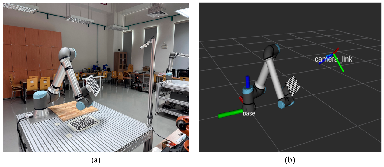
The estimated extrinsic parameters are further validated by visualizing the calibrated camera pose in RViz and comparing it with the real-world robot and camera setup. Using the computed transformation, the camera frame is rendered in the robot coordinate system and shows good alignment with the physical camera placement, as illustrated in Figure 2. This qualitative agreement confirms the correctness of the estimated extrinsic parameters for reliable perception and collision avoidance.

4.3. Human Arm Skeleton Estimation Results

RGB-D frames were acquired at $1280\times 720$ pixels and $30\mathrm{H}\mathrm{z}$, while YOLO26s-pose used an input size of $640$, a detection threshold of 0.25, and a keypoint threshold of $0.35$. Keypoint depth was the median in a $7\times 7$ window and was accepted within 0.25–3.50 m when its local standard deviation was below $0.12 \mathrm{m}$. The constant-velocity Kalman filter used was

$$Q_{KF}=0.035diag\left(∆t^2{I}_3,∆t{I}_3\right),$$

(38)

$$R_{KF}={\displaystyle \frac{0.0025}{max\left(c_{a,j,k},0.05\right)}}{I}_3.$$

(39)

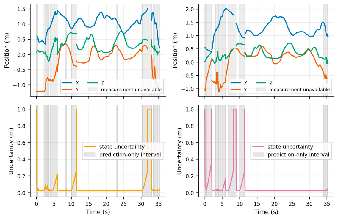
All six diagonal entries of the initial covariance matrix were 0.05. Δt was clipped to 0.001–0.5 s; joint speed and acceleration were limited to 2.5 m s⁻¹ and 8.0 m s⁻²; and prediction-only tracking was limited to 1.5 s. Therefore, the Kalman output is continuous only for dropouts not exceeding 1.5 s. Longer dropouts produce the visible gaps in Figure 3 because the stale track is invalidated and later reinitialized.

For the motion predictor in Section 3.3.4, acceleration was smoothed with $\alpha = 0.15$, the decay coefficient was $\lambda = 2.5 {\mathrm{s}}^{-1}$, and acceleration and jerk were limited to $8.0 \mathrm{m}.{\mathrm{s}}^{-2}$ and $40 \mathrm{m}.{\mathrm{s}}^{-3}$, respectively. The online horizon was $T_P = 0.5 \mathrm{s}$, with future candidates sampled every $0.05 \mathrm{s}$. The robust clearance selection in Equations (27) and (28) used the $35\mathrm{t}\mathrm{h}$ percentile; forecast-only risk required three consecutive frames, and the temporal smoothing weight was $0.15$.

Figure 3 summarizes the estimator response to temporary loss of hand measurements. The longest measurement-unavailable intervals were 2.54 s for the left hand and 2.17 s for the right hand; therefore, only the first 1.5 s of each interval was covered by prediction-only tracking, while the remaining portion appears as a trajectory gap. Across the complete sequence, the left and right hands were in prediction-only mode for 26.8% and 26.6% of the trial, respectively, while total estimate availability reached 96.7% and 97.5%, as shown in

Table 2. Same-sequence comparison of the baseline and integrated proposed configurations.

Metric	Baseline	Proposed
Left-hand availability ($\mathrm{\%}$)	95.3	96.7
Right-hand availability ($\mathrm{\%}$)	87.1	97.5
Left-arm acceleration RMS ($\mathrm{m}.{\mathrm{s}}^{-2}$)	19.00	4.53
Right-arm acceleration RMS ($\mathrm{m}.{\mathrm{s}}^{-2}$)	27.66	4.82
Left-arm jerk RMS ($\mathrm{m}.{\mathrm{s}}^{-3}$)	948.9	179.7
Right-arm jerk RMS ($\mathrm{m}.{\mathrm{s}}^{-3}$)	1509.1	218.3
Robot stopped time ($\mathrm{\%}$)	20.66	7.06
Mean robot speed ($\mathrm{\%}$)	33.95	70.21

. During controlled masking, the RMSE (root mean square error) relative to the withheld RGB-D/YOLO26s-pose keypoint observations was 0.292 m for the left hand and 0.167 m for the right hand.

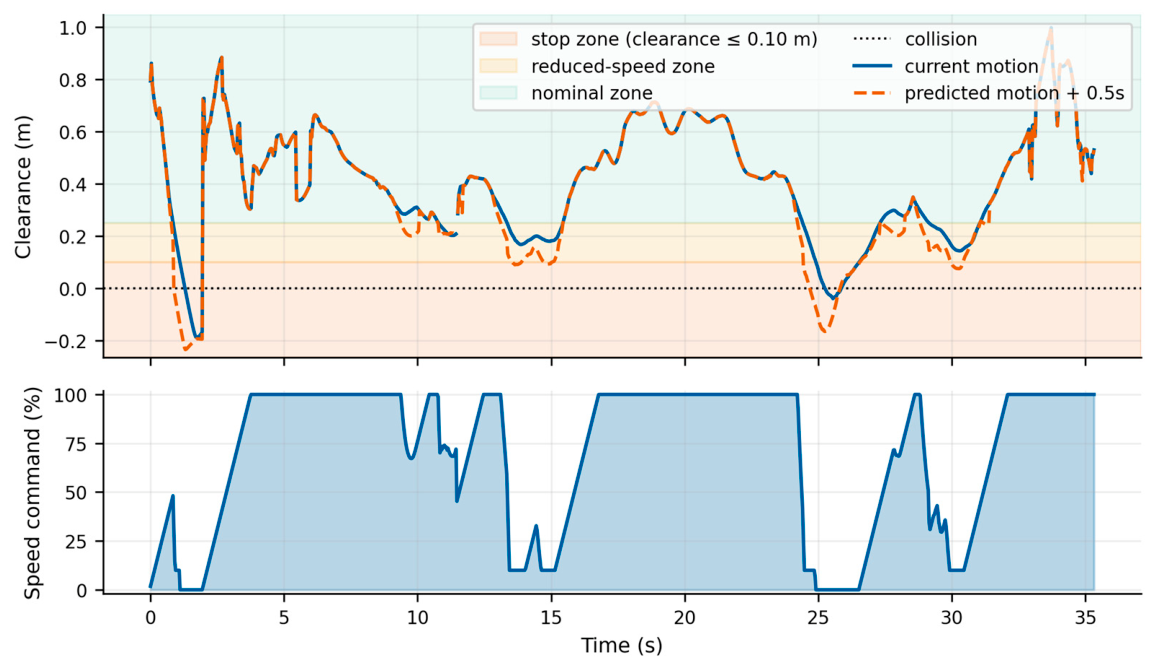
Figure 4 illustrates the time-resolved safety response of the proposed human–robot separation-monitoring framework. The upper panel reports the current hand–robot clearance and the predicted clearance over the short-term motion horizon, while the lower panel shows the corresponding protective robot speed command. The shaded regions define the operational safety bands: collision/overlap at zero clearance, the stop zone below $0.10 \mathrm{m}$, the reduced-speed zone between $0.10 \mathrm{m}$ and $0.25 \mathrm{m}$, and the nominal-speed region above $0.25 \mathrm{m}$.

The predicted clearance generally follows the current clearance trend while anticipating several impending reductions in separation. When the predicted trajectory enters the reduced-speed or stop zone, the controller decreases the commanded robot speed before or during the corresponding close-proximity event. Across the trial, the minimum current clearance reached approximately $-0.190 \mathrm{m}$, while the minimum predicted clearance reached $-0.234 \mathrm{m}$, indicating that the forecasting module produced a more conservative estimate of the closest approach. The system spent approximately $31.7\mathrm{\%}$ of the trial in the warning-or-danger region and $12.1\mathrm{\%}$ in the stop region, while the robot was commanded to stop for approximately $7.1\mathrm{\%}$ of the trial. The mean commanded robot speed was approximately $70.2\mathrm{\%}$, showing that the controller did not simply stop the robot continuously, but modulated the trajectory speed according to the estimated separation risk.

Several intervals show overlap between the current and predicted clearance curves. This occurs when the forecasted future clearance is not confirmed as more hazardous than the current state, or when the current clearance remains the limiting safety condition. In these cases, the stabilized prediction output intentionally follows the current clearance to avoid spurious forecast-induced oscillations. Therefore, the overlap should be interpreted as a conservative stabilization behavior rather than a failure of the prediction module.

Overall, Figure 4 shows that the integrated framework converted predicted human–robot proximity into a continuous protective speed response in the tested sequence. The robot maintained nominal speed when sufficient separation was available, slowed in the warning region, and stopped during confirmed high-risk intervals. This result supports proof-of-concept feasibility under the controlled laboratory conditions; it does not demonstrate superiority to other forecasting methods or readiness for unrestricted industrial deployment.

Table 2 compares the direct RGB-D baseline with the integrated proposed configuration. Left-hand availability increased from 95.3% to 96.7% (1.4 percentage points), and right-hand availability increased from 87.1% to 97.5% (10.4 percentage points). The left- and right-arm acceleration RMS values decreased by 76.2% and 82.6%, respectively, while the corresponding jerk RMS values decreased by 81.1% and 85.5%. These results show greater continuity and temporal stability for the complete proposed pipeline. Because Kalman propagation, kinematic constraints, reconstruction, and stabilization operate together, the comparison does not isolate their independent contributions.

In the integrated comparison, greater trajectory continuity coincided with less conservative controller behavior. The proportion of robot stopped time decreased from 20.66% to 7.06%, while the mean robot speed command increased from 33.95% to 70.21%. These are system-level outcomes under the same tested sequence and should not be attributed quantitatively to any single estimation, prediction, or constraint module.

4.4. Controlled Occlusion Recovery Comparison and Interpretation Limits

Table 3. Robustness to controlled bilateral arm occlusion at different human motion speeds.

Hand Speed (m/s)	Occlusion 1.0 s		Occlusion 1.5 s
	ZOH RMSE (m)	Proposed RMSE (m)	ZOH RMSE (m)	Proposed RMSE (m)
0.397	0.128	0.072	0.300	0.105
0.650	0.212	0.197	0.283	0.265
0.904	0.353	0.284	0.383	0.282

evaluates controlled bilateral elbow/wrist measurement loss in three selected motion speed cases. ZOH (zero-order hold) denotes a non-predictive last-valid-observation hold, whereas the proposed method uses CV-Kalman state propagation with shoulder-anchored distal-arm reconstruction. The direct no-filter pipeline produces no distal skeleton during the bilateral mask and, therefore, has an undefined reconstruction RMSE; ZOH is used as a numerical non-predictive reference.

At the nominal 1.0 s occlusion duration, the proposed pipeline reduced the RMSE from 0.128 to 0.072 m in the low-speed case, from 0.212 to 0.197 m in the medium-speed case, and from 0.353 to 0.284 m in the high-speed case. At 1.5 s, the corresponding values decreased from 0.300 to 0.105 m, from 0.283 to 0.265 m, and from 0.383 to 0.282 m. The unweighted mean RMSE decreased from 0.231 to 0.184 m for the 1.0 s mask and from 0.322 to 0.217 m for the 1.5 s mask. These controlled cases show that the implemented state propagation pipeline outperformed the static zero-order-hold reference when the arm continued to move during synthetic measurement loss. The reference was the same-sequence RGB-D/YOLO26s-pose skeleton retained before masking; thus, RMSE measures trajectory consistency rather than absolute motion capture accuracy. No alternative motion prediction algorithms were tested, so these results do not establish superiority over existing prediction methods.

The safety distance threshold and prediction horizon were selected based on measured human arm velocity and RGB-D tracking uncertainty. The evaluated hand speeds were 0.397, 0.650, and 0.904 $(\mathrm{m}/\mathrm{s})$, with an average of 0.650 $(\mathrm{m}/\mathrm{s})$. Over the selected 0.5 s prediction horizon, the corresponding hand displacements were approximately 0.199, 0.325, and 0.452 m, allowing the system to anticipate motion toward the 0.25 m warning zone.

The 0.25 m threshold was chosen as a conservative engineering margin that accounts for local depth uncertainty and human motion during system response. With a local depth consistency limit of 0.12 m, the remaining 0.13 m corresponds to approximately 0.20 s of hand motion at the average speed. The mean reconstruction RMSE increased from 0.184 m at 1.0 s to 0.217 m at 1.5 s. Therefore, the selected parameters represent a practical compromise between early intervention, prediction uncertainty, and unnecessary robot interruption.

4.5. Human–Robot Safety Response

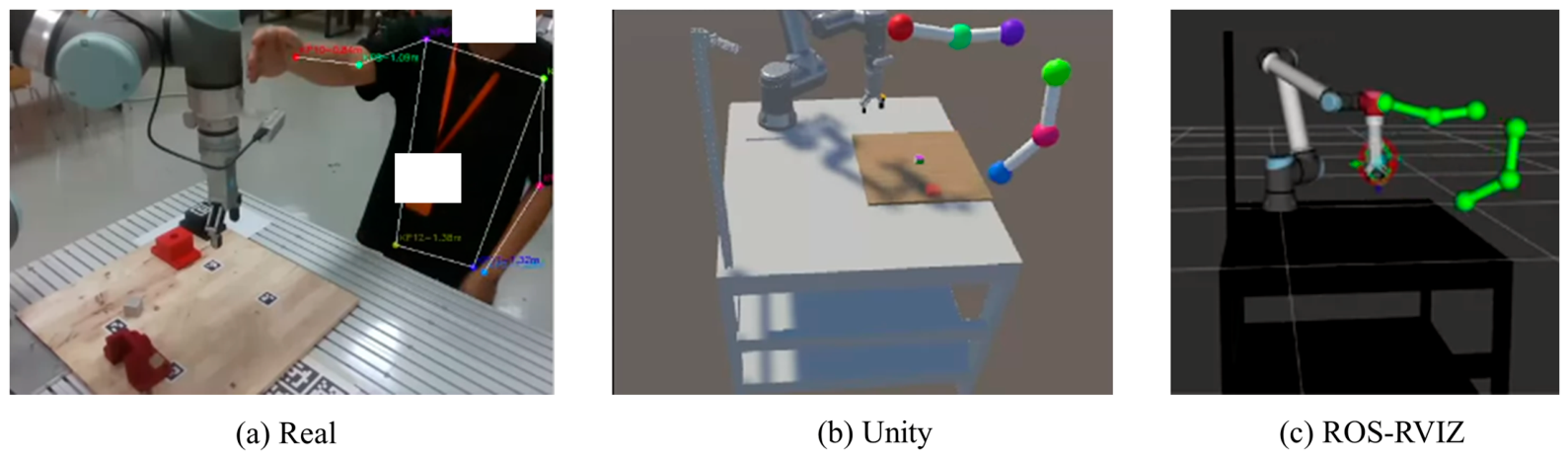
The proposed system’s real-time human–robot distance monitoring is illustrated in Figure 5 using both real and virtual views. In the real view in Figure 5a, the UR10e robot is moving along a planned path when a human arm enters the robot’s workspace and blocks part of its motion. The system detects keypoints of the human arm using a vision-based pose estimation method, and these keypoints are displayed on the real image. The keypoints are tracked continuously and converted into the robot’s coordinate system using the calibrated camera–robot relationship. The three-dimensional positions of the human arm joints are then used to measure the distance between the human and the robot, allowing the system to stay aware of the human’s position while the robot arm is operating.

The synchronized virtual views of the human–robot interaction are shown in Figure 5b,c. In Figure 5b, the Unity-based digital twin displays the UR10e and the human arm using three arm keypoints. Figure 5c shows the ROS/RViz environment, in which human–robot distance is monitored during the experiment. For this proof of concept, the safety threshold was configured as 0.25 m using the engineering rationale described in Section 4.4. Because ROS communication and actuator response latencies were not recorded separately, the threshold should not be interpreted as a formally validated industrial safety distance. When the measured distance fell below the threshold, the nearest robot joint was marked in red, and a stop command was triggered. This experiment verifies information exchange among the physical robot, digital twin, and control system under the tested conditions.

4.6. Reactive Motion Control and Collision Avoidance

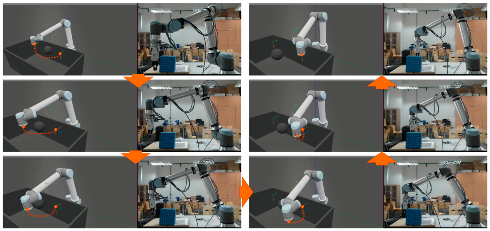
Figure 6 compares the simulated manipulator motion with execution on the physical UR10e under the implemented optimization-based controller. Each row represents a stage of the motion sequence. In simulation, the dotted red arc indicates the trajectory generated by the QP solver around the modeled obstacle. The virtual obstacle is shown as a black sphere, whereas the physical experiment uses a blue cube with an equivalent collision volume in the optimization model. The paired images provide qualitative evidence that the planned avoidance behavior was reproduced by the physical robot in this controlled trial.

Across the illustrated stages, the controller modified the joint velocities as the end-effector approached the modeled obstacle and then redirected the motion toward the task goal after the obstacle was bypassed. The qualitative agreement between simulation and physical execution supports the feasibility of the optimization formulation for the tested trajectory. However, this single controlled sequence does not establish reliability, real-time deployment readiness, or safety performance in unstructured industrial environments.

4.7. Integrated Configuration Comparison and Computational Latency Evaluation

To quantify the incremental computational cost of short-term motion forecasting, the online perception–prediction pipeline was evaluated with forecasting disabled and enabled while all other stages were retained. This is a two-configuration forecasting comparison, not a full module-by-module ablation. The QP/NEO trajectory was generated offline before the collision avoidance algorithm was activated; its computation time was, therefore, outside the online perception–prediction cycle.

Table 4. Per-stage computational latency of the proposed framework with and without short-term motion forecasting. Online stage values and the separately measured offline QP/NEO trajectory generation time are reported as means ± standard deviation in milliseconds.

Processing Stage	Without Forecasting (ms)	With Forecasting (ms)
YOLO26s-pose inference	6.91 ± 0.38	6.91 ± 0.38
3D reconstruction, kinematic constraints, and Kalman filtering	2.96 ± 0.12	3.00 ± 0.08
Clearance evaluation and short-term motion prediction	1.30 ± 0.09	14.64 ± 0.22
QP/NEO trajectory generation (offline; excluded from online subtotal)	85.10 ± 28.13	85.10 ± 28.13
Sum of online stage means (excluding offline QP/NEO and ROS communication)	11.17	24.55

Note: The online subtotal is the arithmetic sum of the three online stage means and excludes offline QP/NEO trajectory generation and ROS communication. A total standard deviation is not reported because full-cycle latency was not measured directly.

reports the online per-stage times measured on the workstation in Section 4.1 and lists the offline QP/NEO trajectory generation time separately.

The online subtotal was 11.17 ms without forecasting and 24.55 ms with forecasting. The 13.38 ms increase was dominated by clearance evaluation and short-term motion prediction, whose mean processing time increased from 1.30 to 14.64 ms. These online computational subtotals correspond to nominal update rates of approximately 89.5 Hz and 40.7 Hz, respectively. Although the 24.55 ms subtotal with forecasting is below the 33.33 ms period of a 30 Hz camera stream, complete end-to-end operation at 30 Hz cannot be established without measuring ROS communication, robot command reception, and actuator response latency. The separately measured QP/NEO value of 85.10 ± 28.13 ms represents offline trajectory generation performed before the collision avoidance algorithm was activated and is, therefore, not included in either online subtotal.

The existing results, nevertheless, provide quantitative evidence for estimation smoothness and robustness under occlusion and rapid human motion. As shown in Table 2, the proposed method reduced the left- and right-arm acceleration RMS from 19.00 and 27.66 m·s⁻² to 4.53 and 4.82 m·s⁻², respectively, and reduced the corresponding jerk RMS from 948.9 and 1509.1 m·s⁻³ to 179.7 and 218.3 m·s⁻³. These indicators describe the temporal smoothness of the reconstructed human arm trajectory, rather than the physical end-effector trajectory. Furthermore, Table 3 evaluates controlled 1.0 s and 1.5 s bilateral arm occlusions at hand speeds of 0.397, 0.650, and 0.904 m·s⁻¹. Therefore, the current evidence supports the robustness of the perception and prediction pipeline to temporary occlusion and increasing human motion speed, but it should not be interpreted as a task-level robot success rate evaluation.

The present experiments did not separately record ROS communication, robot command reception, or actuator response latency. Accordingly, the online values in Table 4 are computational subtotals rather than complete sensor-to-actuator latency. The reported QP/NEO time is an offline trajectory generation measurement and does not represent an online controller delay. Moreover, the available dataset does not provide independent measurements of end-effector positioning accuracy, physical end-effector trajectory smoothness, task completion time, task-level success rate, or performance under varying illumination. These quantities cannot be reconstructed reliably from the available data and require dedicated experiments.

The tight coupling among Kalman filtering, kinematic constraints, short-term prediction, clearance evaluation, and control also prevents the present comparisons from quantifying each module’s independent contribution. The forecasting experiment isolates only the difference between enabled and disabled forecasting, and no alternative prediction algorithms were evaluated. Therefore, all performance claims are restricted to the compared integrated configurations. Finally, the experiments were conducted in a controlled, primarily single-participant laboratory setting and should be interpreted as feasibility validation rather than comprehensive industrial safety validation.

5. Conclusions and Future Work

This study presented a digital twin-based framework that integrates RGB-D pose estimation, Kalman-based 3D arm tracking, short-term motion prediction, predicted-clearance evaluation, and an offline-generated QP/NEO trajectory. Under controlled laboratory conditions, the integrated framework maintained hand trajectories during temporary measurement loss, anticipated reductions in human–robot separation, and triggered graded speed reduction or stopping. The online computational subtotal was 24.55 ms with forecasting and 11.17 ms without forecasting, excluding offline QP/NEO trajectory generation, ROS communication, robot command reception, and actuator response; these values are not complete sensor-to-actuator latencies. Because the compared stages are tightly coupled, the results do not quantify the independent contributions of Kalman filtering, kinematic constraints, prediction, or control. The prediction results are limited to no-prediction and zero-order-hold references and do not demonstrate superiority over other prediction methods. Accordingly, this study establishes proof-of-concept feasibility rather than industrial deployment readiness. Future work will evaluate alternative predictors and conduct factorial module ablations where technically feasible. It will also use independent motion capture and robot controller measurements to assess end-effector accuracy, physical trajectory smoothness, task completion time, task-level success rate, and complete end-to-end latency in more complex industrial environments with multiple participants, dynamic occlusion, varying illumination, and rapid human motion.

References

1. Schulman, J.; Duan, Y.; Ho, J.; Lee, A.; Awwal, I.; Bradlow, H.; Pan, J.; Patil, S.; Goldberg, K.; Abbeel, P. Motion Planning with Sequential Convex Optimization and Convex Collision Checking. Int. J. Robot. Res. 2014, 33, 1251–1270. [Google Scholar] [CrossRef] [Scilit]
2. Xia, G.; Ghrairi, Z.; Wuest, T.; Hribernik, K.; Heuermann, A.; Liu, F.; Liu, H.; Thoben, K.-D. Towards Human Modeling for Human-Robot Collaboration and Digital Twins in Industrial Environments: Research Status, Prospects, and Challenges. Robot. Comput.-Integr. Manuf. 2025, 95, 103043. [Google Scholar] [CrossRef] [Scilit]
3. Jung, K.; Yang, J.-S. Mitigating Safety Challenges in Human-Robot Collaboration: The Role of Human Competence. Technol. Forecast. Soc. Change 2025, 213, 124022. [Google Scholar] [CrossRef] [Scilit]
4. Liu, S.; Liu, Z.; Qin, Q.; Wang, X.V.; Wang, L. Multimodal Human-Robot Collaboration: Advancements and Future Directions. Int. J. Manuf. Res. 2025, 20, 1–47. [Google Scholar] [CrossRef] [Scilit]
5. Villani, V.; Pini, F.; Leali, F.; Secchi, C. Survey on Human–Robot Collaboration in Industrial Settings: Safety, Intuitive Interfaces and Applications. Mechatronics 2018, 55, 248–266. [Google Scholar] [CrossRef] [Scilit]
6. Grieves, M.; Vickers, J. Digital Twin: Mitigating Unpredictable, Undesirable Emergent Behavior in Complex Systems. In Transdisciplinary Perspectives on Complex Systems; Kahlen, J., Flumerfelt, S., Alves, A., Eds.; Springer: Cham, Switzerland, 2017; pp. 85–113. [Google Scholar] [CrossRef] [Scilit]
7. Cao, Z.; Simon, T.; Wei, S.; Sheikh, Y. Realtime Multi-Person 2D Pose Estimation Using Part Affinity Fields. In Proceedings of the IEEE Conference on Computer Vision and Pattern Recognition (CVPR), Honolulu, HI, USA, 21–26 July 2017; pp. 7291–7299. [Google Scholar] [CrossRef] [Scilit]
8. Cheng, Y.; Wang, H.; Bao, Y.; Lu, F. Appearance-Based Gaze Estimation with Deep Learning: A Review and Benchmark. IEEE Trans. Pattern Anal. Mach. Intell. 2024, 46, 7509–7528. [Google Scholar] [CrossRef] [Scilit] [PubMed]
9. Lee, J.; Kim, Y.; Kim, S.; Nguyen, Q.; Heo, Y. Learning Fast, Tool-Aware Collision Avoidance for Collaborative Ro-bots. IEEE Robot. Autom. Lett. 2025, 10, 7731–7738. [Google Scholar] [CrossRef] [Scilit]
10. Yoon, J.; Lee, Z. Collision Detection and Body-Part Classification in Collaborative Robots Using a Multi-Task Deep Learning Model with Hybrid Time-Series Augmentation. IEEE Access 2026, 14, 9758–9777. [Google Scholar] [CrossRef] [Scilit]
11. Heo, Y.J.; Kim, D.; Lee, W.; Kim, H.; Park, J.; Chung, W.K. Collision Detection for Industrial Collaborative Robots: A Deep Learning Approach. IEEE Robot. Autom. Lett. 2019, 4, 740–746. [Google Scholar] [CrossRef] [Scilit]
12. Tao, Y.; Li, M.; Cao, X.; Lu, P. Mobile Robot Collision Avoidance Based on Deep Reinforcement Learning with Motion Constraints. IEEE Trans. Intell. Veh. 2025, 10, 2163–2173. [Google Scholar] [CrossRef] [Scilit]
13. Lugaresi, C.; Tang, J.; Nash, H.; McClanahan, C.; Uboweja, E.; Hays, M.; Zhang, F.; Chang, C.-L.; Yong, M.G.; Lee, J.; et al. MediaPipe: A Framework for Building Perception Pipelines. arXiv 2019, arXiv:1906.08172. [Google Scholar] [CrossRef] [Scilit]
14. Lasota, P.A.; Fong, T.; Shah, J.A. A Survey of Methods for Safe Human–Robot Interaction. Found. Trends Robot. 2017, 5, 261–349. [Google Scholar] [CrossRef] [Scilit]
15. Ajoudani, A.; Zanchettin, A.M.; Ivaldi, S.; Albu-Schäffer, A.; Kosuge, K.; Khatib, O. Progress and Prospects of the Human–Robot Collaboration. Auton. Robot. 2018, 42, 957–975. [Google Scholar] [CrossRef] [Scilit]
16. Liao, Z.; Xu, Z.; Xu, X.; Ismail, A. Mean-Shift-Based Moving Target Tracking Algorithm in Complex Industrial Environments. Int. J. Comput. Appl. Technol. 2025, 78, 112–123. [Google Scholar] [CrossRef] [Scilit]
17. Lian, M.; Li, L.; Wang, S.; Wang, C.; Li, M. Design and Research of IIoT Intelligent Automatic Production Line Security Monitoring System Based on Digital Twin. Int. J. Comput. Appl. Technol. 2026, 78, 13–24. [Google Scholar] [CrossRef] [Scilit]
18. Kritzinger, W.; Karner, M.; Traar, G.; Henjes, J.; Sihn, W. Digital Twin in Manufacturing: A Categorical Literature Review and Classification. IFAC-PapersOnLine 2018, 51, 1016–1022. [Google Scholar] [CrossRef] [Scilit]
19. Feng, B.; Wang, Z.; Yuan, L.; Zhou, Q.; Chen, Y.; Bi, Y. Towards Safe Motion Planning for Industrial Human-Robot Interaction: A Co-Evolution Approach Based on Human Digital Twin and Mixed Reality. Robot. Comput.-Integr. Manuf. 2025, 95, 103012. [Google Scholar] [CrossRef] [Scilit]
20. Jocher, G.; Qiu, J.; Liu, M.; Lyu, S.; Akyon, F.C.; Kalfaoglu, M.E. Ultralytics YOLO26: Unified Real-Time End-to-End Vision Models. arXiv 2026, arXiv:2606.03748. [Google Scholar] [CrossRef] [Scilit]
21. Sapkota, R.; Cheppally, R.H.; Sharda, A.; Karkee, M. YOLO26: Key Architectural Enhancements and Performance Benchmarking for Real-Time Object Detection. arXiv 2025, arXiv:2509.25164. [Google Scholar] [CrossRef] [Scilit]
22. Tsai, R.Y. A Versatile Camera Calibration Technique for High-Accuracy 3D Machine Vision Metrology Using Off-the-Shelf TV Cameras and Lenses. IEEE J. Robot. Autom. 1987, 3, 323–344. [Google Scholar] [CrossRef] [Scilit]
23. Haviland, J.; Corke, P. NEO: A Novel Expeditious Optimisation Algorithm for Reactive Motion Control of Manipulators. IEEE Robot. Autom. Lett. 2021, 6, 1043–1050. [Google Scholar] [CrossRef] [Scilit]
24. Yoshikawa, T. Manipulability of Robotic Mechanisms. Int. J. Robot. Res. 1985, 4, 3–9. [Google Scholar] [CrossRef] [Scilit]
Figure 1. Overall workflow of the proposed digital twin-based predictive collision avoidance framework.
Robotics 15 00150 g001
Figure 2. Comparison between the real-world setup and the estimated camera pose after extrinsic calibration. (a) Real-world camera and robot setup; (b) estimated camera pose visualized in RViz.
Robotics 15 00150 g002
Figure 3. Kalman-based temporary occlusion handling for 3D hand tracking. The upper row shows filtered hand position; gray intervals denote unavailable measurements. The lower row shows state uncertainty during prediction-only tracking. Gaps occur when measurement loss exceeds the 1.5 s prediction timeout.
Robotics 15 00150 g003
Figure 4. Predictive human–robot clearance and protective speed response. The upper panel shows the current and predicted hand–robot clearance with safety regions, while the lower panel reports the resulting robot speed command.
Robotics 15 00150 g004
Figure 5. Real and virtual views of keypoint detection, proximity monitoring, and robot stopping at the safety threshold: (a) physical scene; (b) Unity environment; and (c) ROS/RViz environment.
Robotics 15 00150 g005
Figure 6. Comparison between simulation (left) and real robot execution (right) during reactive motion control. The optimization-based controller computes collision-free joint velocities that follow the desired task trajectory (red dotted curve) while avoiding the obstacle. Orange arrows indicate the progression of time from the initial state (top left) to the final state (top right).
Robotics 15 00150 g006