Article

Flexipede: A Bio-Inspired, Modular Myriapod Robot for Rough-Terrain Traversal

Department of Robotics and Mechatronics Engineering, University of Dhaka, Dhaka 1000, Bangladesh
*
Author to whom correspondence should be addressed.
These authors contributed equally to this work.
Robotics 2026, 15(7), 129; https://doi.org/10.3390/robotics15070129
Submission received: 1 May 2026 / Revised: 5 June 2026 / Accepted: 9 June 2026 / Published: 1 July 2026
(This article belongs to the Section Intelligent Robots and Mechatronics)

Abstract

Rough-terrain exploration is critical for applications ranging from post-disaster search-and-rescue to planetary exploration. While conventional wheeled or bipedal robots often struggle in these environments, biological organisms like myriapods demonstrate superior adaptability. Inspired by this, we present Flexipede—a compact, modular robotic system that employs a hybrid actuation architecture, wherein each module integrates a single actuator for propulsive gait generation and a secondary actuator to enable distributed yaw control. The platform is fully 3D-printable and cost-effective, with a fabrication cost of approximately $58 for the primary unit and $10 per additional module. Analytical kinematic modeling was employed to optimize linkage trajectories, with experimental results validating the system across six modular configurations and three distinct environments, including flat, rough, and inclined terrains. The platform achieved locomotion speeds up to 9 cm/s and navigated obstacles up to 32 mm high, while linkage path deviations remained functionally negligible (mean deviation of 3.24 % ) compared to analytical prediction. Turning performance converged with theoretical predictions as modular scaling increased, reaching a minimum deviation of 4.51 % for the five-module configuration. Across all terrains, the system maintained a competitive average Cost of Transportation (CoT) of 18.01 , with stair climbing requiring a relatively higher CoT due to the elevated torque demands associated with vertical displacement. These results establish Flexipede as a high-performance benchmark for modular myriapod systems with significant potential for adaptive morphological research.

1. Introduction

In numerous real-world scenarios, such as disaster rescue, underground search, and mining missions, operations must be conducted across highly irregular terrains characterized by loose soil, rubble, pebbles, and debris. Because these scenarios often present extreme hazards or physical limitations for human personnel, robotic systems serve as the most viable alternative [1,2]. To be effective, these robots must maneuver swiftly and reliably across unpredictable terrain to provide timely assistance, collect critical data, or deliver essential supplies.
Various studies have explored diverse robotic locomotion methods for effective operation in rough terrains. Among them, wheeled robots offer mechanical simplicity, but frequently suffer from instability, slippage, and poor performance on irregular topographies [3,4,5]. As an alternative, aerial drones enable the rapid exploration of complex environments; however, limited power capacity and fragile structures severely restrict their endurance and operational reliability [6,7]. In contrast, legged systems offer superior terrain adaptability. For instance, bipedal robots have demonstrated effective traversal capabilities [8,9,10], with simplified, low-cost single-actuator systems proven viable in [11] and [12]. Notably, Zippy [13]—the smallest autonomous biped to date—demonstrated high speed (25 cm/s or 10 leg-lengths per second(LL/s)) and efficiency (CoT of 11.2) compared to other compact platforms like Mugatu (1.05 LL/s) [11], Collins et al. (0.54 LL/s) [14].
Despite their agility, bipedal robots struggle greatly with instability on rough terrain [13,15,16]. Consequently, multipedal robots, including biomimetic myriapod robots, have been developed to ensure stable, adaptive locomotion [8,15,17,18]. By leveraging many legs and maneuverable bodies, these systems handle rough terrain efficiently. However, balancing mechanical complexity with high performance remains a challenge. For instance, Torige’s centipede robot [3], Aoi’s flexible 12-legged robot [15], Ozkan-Aydin’s hybrid myriapod [19], Hou’s modular rescue robot [20], and Hoffman’s three-segment microrobot [21] successfully achieved stable multi-legged coordination. However, they relied on high actuator densities (up to four actuators per module), which increased system weight and restricted velocities (e.g., Torige’s platform achieved only 0.86 cm/s). Conversely, Koh’s centipede robot [8] utilized a centralized single-actuator mechanism, enabling the full robot to reach higher velocities of 6.8 to 8.9 cm/s, though with limited modular adaptability. Other approaches, such as Yin’s and Yasui’s, utilized central pattern generators for decentralized gait control [17,18]. While some recent iterations integrated AI and modularity for search-and-rescue or agricultural applications, they are primarily restricted to flat environments [20,21,22,23]. Crucially, however, none of the aforementioned platforms report their Cost of Transport (CoT), leaving their practical energetic viability unquantified. Moreover, the aforementioned platforms also failed to report quantitative analysis regarding stair-climbing capabilities.
Existing studies on myriapod-inspired robots typically employ multiple actuators per module, necessitating complex coordination strategies and high computational overhead [8,15,16,18]. This elevated actuator density increases design complexity, fabrication costs, and overall system weight while often limiting modular flexibility to fixed segment counts [4,5,8,15,24,25,26,27,28]. To address these challenges, this study presents Flexipede, a modular myriapod-inspired robot featuring a single-actuator-driven bipedal mechanism per module supplemented by a servo-driven active-yaw steering connector that enables rapid reconfiguration and scaling according to operational needs. The major contributions of this work include the following: (1) the design and development of a single-actuator driven bipedal linkage and a servo-driven reconfigurable inter-module coupling mechanism; (2) the derivation of an analytical kinematic model of the developed bipedal mechanism and validation against physical prototypes; (3) experimental evaluation across an extensive range of modular configurations (n = 1 to 6) and environments; and (4) the establishment of a Cost of Transport (CoT) benchmark for myriapod-inspired platforms.
The remainder of this paper is organized as follows: Section 2 details the materials and methodology applied in this work. Section 3 presents the experimental evaluation and analysis, while Section 4 discusses the implications of these results in detail. Finally, Section 5 concludes the paper with a summary of the main contributions, current limitations, and future research directions.

2. Materials and Methods

The design of the Flexipede was bio-inspired, emulating the segmented morphology of myriapods to achieve a modular, scalable architecture. The system incorporated a custom bipedal mechanism for individual module locomotion alongside a specialized inter-module connector for structural expansion. Actuation was managed by an embedded electrical system, while fabrication employed a cost-effective approach combining 3D printing and off-the-shelf components to facilitate rapid prototyping and accessibility.

2.1. Hardware Design

The robotic hardware was developed with Design for Manufacturing (DFM) principles in mind [29,30]. Components were specifically optimized for 3D printing, leveraging print-in-place techniques where applicable, to ensure that the custom walking mechanisms and inter-module connectors could be efficiently fabricated and assembled.

2.1.1. Walking Mechanism

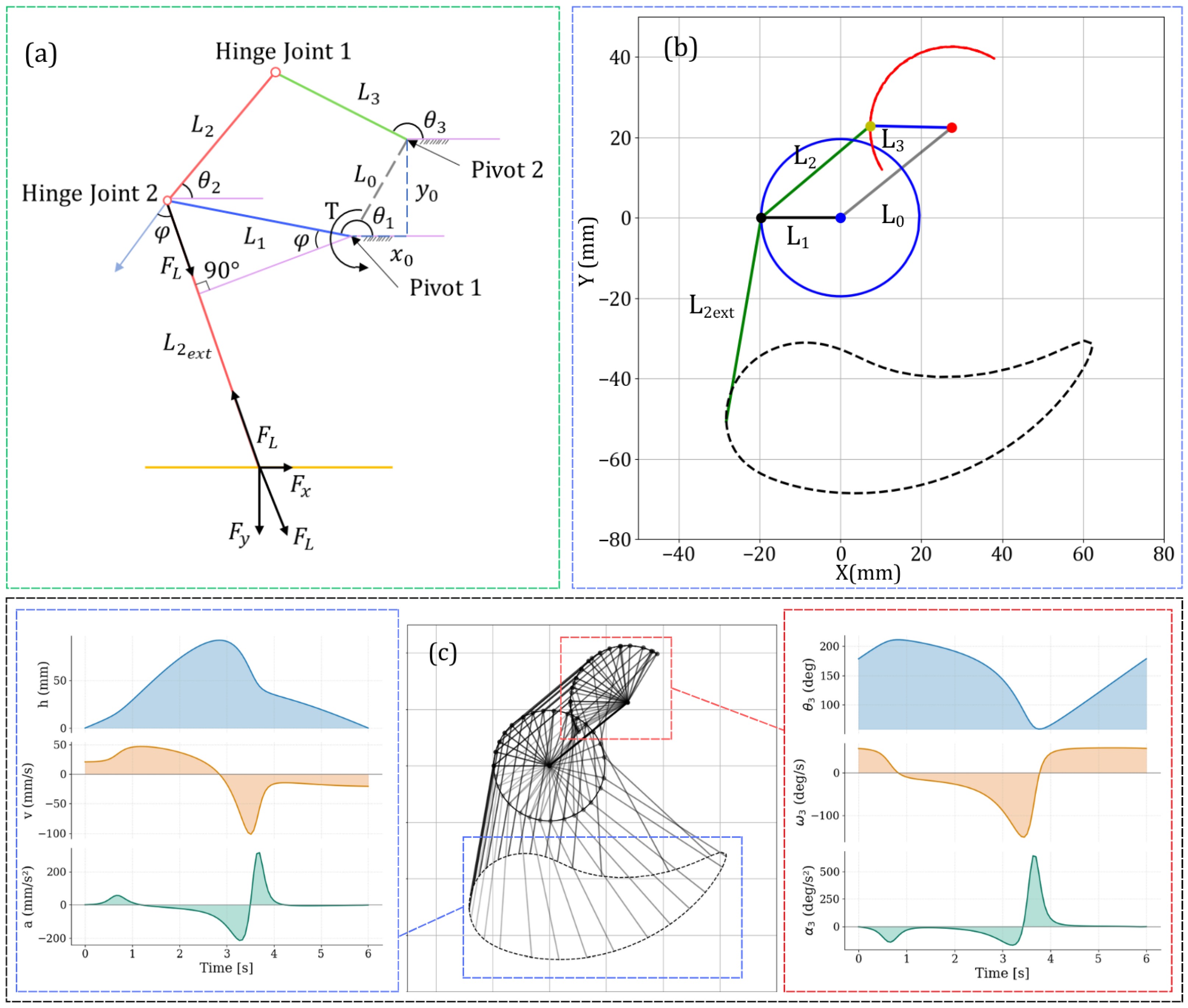
To minimize cost and complexity, the walking mechanism was designed using a single geared DC motor to actuate a planar four-bar linkage. The mechanism consisted of a fixed link, L 0 (integrated into the chassis), and three moving links ( L 1 , L 2 , and L 3 ) (Figure 1a). Links L 1 and L 3 were pinned to L 0 at P i v o t 1 and P i v o t 2 , respectively, while the coupler link ( L 2 ) joined their distal ends to form a closed-loop system. Link L 2 featured an extended, angled segment, L 2 e x t , which functioned as the robot’s leg. P i v o t 1 and P i v o t 2 were separated by L 0 x units horizontally and L 0 y units vertically. During operation, the motor rotated L 1 about P i v o t 1, causing L 2 to trace a specific walking trajectory constrained by the motion of link L 3 (Figure 1b).
To achieve a functional walking gait, the linkage mechanism was designed following two primary kinematic constraints: (i) the distal endpoint of the L 2 e x t segment was required to generate a closed-loop trajectory [31,32], and (ii) this trajectory needed to exhibit greater horizontal extension than vertical displacement [4,33]. In practice, established optimizations for single-actuator linkages prioritize a horizontal stride that exceeds 2 × the vertical step height to maximize forward progression [4]. Since arbitrary link length ratios frequently fail to produce closed loops, usable dimensions ( L 1 , L 2 , and L 3 ) were determined through custom Python (v3.12) kinematic analysis using the Matplotlib library (v3.10.3) (Figure 1c). These analyses applied loop-closure equations to evaluate the coordinates of the joints and the L 2 e x t endpoint [31]. For a given input crank angle θ 1 , the angular positions of the remaining links ( θ 2 and θ 3 ) were defined relative to the horizontal x-axis (measured counter-clockwise) by the following system:
L 1 cos ( θ 1 ) + L 2 cos ( θ 2 ) L 0 X L 3 cos ( θ 3 ) = 0
L 1 sin ( θ 1 ) + L 2 sin ( θ 2 ) L 0 Y L 3 sin ( θ 3 ) = 0
After sweeping through various ratio combinations, the ideal values found were converted to millimeters and scaled to finalize the physical walking mechanism design (Table 1).
As illustrated in Figure 1b,c, links L 2 and L 3 undergo non-circular periodic motion, inherently generating localized peak accelerations at specific phases of the gait cycle. To ensure these inertial loads remained within the structural limits of the 3D-printed components, the system’s kinematic profiles were rigorously analyzed. Figure 1c presents the displacement from the starting position (h), linear velocity (v), and linear acceleration (a) of the L 2 e x t distal tip, alongside the angular displacement ( θ ), velocity ( ω ), and acceleration ( α ) of link L 3 . These profiles were derived by applying a counter-clockwise revolution to the driving crank ( L 1 ) over a 6-s period. The resulting kinematic data confirmed that both translational and angular magnitudes remained within feasible bounds for stable physical implementation, consistent with established locomotion constraints [33,34].
Figure 1. Kinematic modeling and simulation of the walking mechanism. (a) Kinematic model of the four-bar linkage-based walking mechanism. L 1 denotes the driving link, L 2 represents the coupler link with an integrated leg extension ( L 2 e x t ), and L 3 indicates the follower link. The force F L exerted by L 2 e x t on the ground is decomposed into a longitudinal propulsive component ( F x ) and a vertical normal component ( F y ) supporting the system against gravity. The Global reference origin (0,0) for this kinematic model is located at P i v o t 1 . (b) Theoretical trajectory of the leg endpoint ( L 2 e x t ) generated by counter-clockwise (CCW) actuation of L 1 about P i v o t 1 . The gait profile was modeled in Python (v3.12) using the Matplotlib library (v3.10.3) and using the kinematic parameters specified in Table 1. (c) Kinematic analysis of the mechanism over one complete cycle. For the L 2 e x t endpoint, h, v, and a denote displacement, linear velocity, and linear acceleration, respectively. For link L 3 , angular displacement ( θ ), angular velocity ( ω ), and angular acceleration ( α ) about P i v o t 2 are plotted against time. The continuity and bounded magnitudes of these profiles validate the mechanical feasibility and physical implementability of the design [31,33].
Robotics 15 00129 g001
To quantify the interaction between the mechanism and the walking surface, the relationship between the input motor torque, T i n , and the resultant ground reaction forces was established. As illustrated in Figure 1a, a counter-clockwise torque T i n was applied to the driving link L 1 at P i v o t 1. Under the assumption that L 2 e x t acted as a rigid two-force member [12,33] subjected to a compressive load F L , the relationship between the applied torque and this internal force was defined as
T i n = F L · L 1 cos ( ϕ ) F L = T i n L 1 cos ( ϕ )
In this expression, ϕ represents the angle between the driving link L 1 and the line perpendicular to L 2 e x t passing through P i v o t 1. Geometrically, this angle was expressed as ϕ = θ 2 θ 1 + 130 ° , where θ 2 was derived by solving the loop-closure equations presented in Equations (1) and (2).
By assuming quasi-static equilibrium [16,25], the force F L was considered to be transmitted directly to the ground. The horizontal ( F L x ) and vertical ( F L y ) components of this force were determined based on the orientation of the leg segment, θ L (defined as the angular displacement from the x-axis), where θ L = θ 2 + 40 ° :
F L x = T i n cos ( θ L ) L 1 cos ( ϕ )
F L y = T i n sin ( θ L ) L 1 cos ( ϕ )
The longitudinal component, F L x , represented the propulsive force driving the robot forward, while the vertical component, F L y , represented the normal force supporting the system’s weight against gravity. By analyzing these components, the mechanical efficiency and weight-bearing capacity of the Flexipede architecture were evaluated across the full gait cycle.
The mechanism was modeled in Autodesk Fusion [4,18,23] using the dimensional parameters specified in Table 1. To form the bipedal configuration, the assembly was mirrored with a 180° angular offset relative to θ 1 , as illustrated in Figure 2a. Both linkages were coupled via a common primary shaft, which transmitted rotational torque from the motor to both L 1 driving links. This centralized actuation scheme facilitated the operation of both legs using a single DC motor. A spur gear was mounted on the primary shaft to interface with the motor’s output, which featured a pinion gear with a 2:1 reduction ratio. This configuration provided a mechanical advantage to increase torque delivery [27,34]. The selection of the 2:1 ratio was dictated by the available physical space. Additionally, a protective chassis was designed to enclose the walking mechanism while providing sufficient internal volume for the integrated electronics.

2.1.2. Inter-Module Coupling Mechanism

An active inter-module coupling mechanism was developed to facilitate controlled rotational articulation about the vertical (yaw) axis between adjacent segments (Figure 2b). The assembly comprised a servo-driven spur gear mounted on the trailing module, which interfaced with a corresponding partial spur gear integrated into the chassis of the preceding segment. Torque applied to the trailing gear governed the yaw angle of the leading module, thereby enabling coordinated steering and multi-directional maneuvering. The preceding module articulated around a central pivot shaft housed within a receptacle on the trailing module. To maintain structural integrity during locomotion, axial displacement of the pivot shaft was constrained by a mechanical retaining clip secured with M3 fasteners. This configuration ensured a robust mechanical connection while allowing for the requisite degrees of freedom for complex gait trajectories.
To evaluate the maneuverability of the robot across various modular configurations, the radius of curvature of the trajectory was estimated as a function of the total number of modules. This estimation was formulated using analytical coordinate geometry, where directional vectors were established for each constituent module (Figure 2c).
For the derivation, the trailing module was positioned at the origin ( 0 , 0 ) , with its orientation defined along the vertical axis (represented by the line segment O A ). Consequently, the direction line for the first module was defined by x = 0 . Each subsequent module advanced a linear distance L—corresponding to the module length—before undergoing a relative rotational deviation of angle α with respect to the heading of the preceding module. For the second module, a rotation of α yielded the direction line:
y L = x cot α
As the sequence continued, the third module underwent an additional angular displacement of α after traversing the forward distance L. The direction line for the third module was thus expressed as follows:
( y L L cos α ) = ( x L sin α ) cot 2 α
By generalizing this kinematic path through successive linear transitions L and constant angular displacements α , the terminal directional vector was established for an arbitrary number of modules, n (where n { 3 , 4 , 5 , } ). The direction line for the n-th module was defined as follows:
y L k = 1 n 2 L cos ( k α ) = x k = 1 n 2 L sin ( k α ) cot ( ( n 1 ) α )
To facilitate further calculation, this n-th module direction line was simplified into the standard slope-intercept form, y = m x + C . By isolating the variables in Equation ((8)), the slope (m) and the y-intercept (C) were defined as
m = cot ( ( n 1 ) α )
C = L + k = 1 n 2 L cos ( k α ) cot ( ( n 1 ) α ) k = 1 n 2 L sin ( k α )
The trajectory was subsequently modeled as a circular arc. Given that the path passed through the origin ( 0 , 0 ) and the initial direction line ( x = 0 ) served as a tangent, the equation for the circular trajectory can be expressed as ( x R ) 2 + y 2 = R 2 . Finally, by utilizing the n-th module’s direction line as the terminal tangent to this circle, the overall radius of curvature, R, was derived. This geometric relationship yielded
R = m C + C m 2 + 1
Using Equation (11), the theoretical radius R could be calculated for any specified modular configuration and joint angle α . In the current design, the maximum articulation angle was constrained to α m a x = 25°. Based on Equations (9)–(11), the robot’s n rigid modules at maximum bending form a regular polygon that circumscribes a minimum-radius incircle. To prevent head–tail self-collision, the total body arc length of Flexipede must not exceed this polygon’s perimeter. Applying this geometric boundary condition and using the platform parameters L = 105.7 mm and α = 25° establishes a maximum theoretical limit of n = 18 modules for Flexipede. The detailed mathematical derivation for this maximum theoretical module count is provided in Appendix B.

2.1.3. Prototype Iterations

The robotic system was developed through eight design iterations, culminating in functional configurations ranging from one to six modules. The modular architecture, complemented by a screw-based assembly approach, facilitated rapid design modifications, maintenance, and component replacement.
Initial kinematic failures—stemming from print-in-place part fusion [34], linkage dimensional errors, and suboptimal coupling of the P i v o t 2 shaft—were resolved through geometric refinement and shaft excision. Subsequent trajectory deviations, resulting from excessive joint clearances and stochastic transitions between planar four-bar assembly modes, were mitigated by implementing tighter tolerances and mechanical hard stops (Figure 2b). Finally, dynamic instability caused by an elevated center of mass was corrected by widening the chassis footprint, thereby ensuring robust locomotion and directional maneuverability.

2.1.4. Electrical and Control Systems

The control architecture of the robotic system was centered around the Seeed Studio XIAO ESP32-C3 microcontroller (Seeed Studio, Shenzhen, China). This platform was selected for its integrated Wi-Fi capabilities, a 160 MHz clock speed providing sufficient processing power for real-time control [35], and a compact form factor (21 × 17.5 mm). In the current design, a single microcontroller governs the entire system, utilizing native Wi-Fi functionality to enable wireless communication via a locally hosted web-based control interface.
For primary locomotion, modified MG90S servo motors (Generic, Shenzhen, China) were selected for their high torque output (2.2 kg·cm at 6 V). The modifications involved removing the internal potentiometer to disable position feedback and eliminating physical mechanical stops to allow continuous 360° rotation. This modification enabled bidirectional speed and directional control via Pulse Width Modulation (PWM) signals from the ESP32 (Espressif Systems, Shanghai, China). Conversely, for active yaw control within the inter-module connectors, unmodified MG90S servos were utilized. By leveraging the integrated H-bridge driver within the MG90S, external circuit complexity was reduced, conserving space within the compact modules.
To balance high energy demands with strict spatial constraints, a custom 7.4 V, 5000 mAh Lithium-ion battery pack was fabricated by connecting two Samsung INR21700-50S cells (Generic, Shenzhen, China) in series. Power was routed to the actuators via a custom-built power distribution board. The battery pack was calculated to provide an operational runtime ranging from 1.57 h to 15.35 h, depending on terrain resistance and the number of active modules. However, to simplify testing procedures and isolate mechanical performance during this study, the robot was powered via an external supply and controlled using a Hiwonder 6-Channel Digital Servo Controller (Hiwonder, Shenzhen, China) rather than the onboard battery and microcontroller. It should be noted that a regulated external supply maintains a stiff terminal voltage regardless of load, whereas the onboard lithium-ion pack exhibits voltage sag under high current draw; the energetic implications of this distinction, along with the added mass of the onboard power supply, are quantified in Appendix A.

2.2. Fabrication

The physical modules were fabricated via Fused Deposition Modeling (FDM) utilizing Bambu Lab X1-Carbon (Bambu Lab, Shenzhen, China) and Elegoo Neptune 4 Max (Elegoo, Shenzhen, China) 3D printers. G-code was generated using the open-source slicing software OrcaSlicer (version 2.3.0, Open-source community) [36]. A print-in-place technique [34] was employed to streamline the assembly of the multi-linkage system and minimize manual post-processing requirements. Polylactic Acid (PLA) was selected as the primary structural material due to its high tensile strength (38.7 MPa) and rigidity (3187 MPa) [37]. Given its high Young’s modulus (1538 MPa) and low elongation at break (4.5–10.6%), PLA provided the requisite structural stiffness to prevent mechanical deformation, which is critical for maintaining precise linkage kinematics [38,39].
Components were printed using a 0.4 mm nozzle on textured Polyetherimide (PEI) build plates [37], with a nozzle temperature of 220 °C and a bed temperature of 60 °C. Final module assembly was completed using hot-melt adhesive and standard M3 fasteners.
Following mechanical assembly, the electrical architecture was integrated into the chassis. To enhance ground traction, rubber pads were adhered to the contact regions of each leg endpoint. As detailed in Table 2, the total production cost for the primary module (including the control system and power source) was $58.00, with an incremental cost of $10.00 for each subsequent module.

2.3. Experimental Protocol

To quantitatively evaluate the performance and maneuverability of the robotic system, a series of experiments was conducted using multiple modular configurations across various environments. For all experimental trials, the robot was powered by an external regulated DC power supply maintained at 5 V ( ± 5 % ) to ensure consistent motor torque and speed profiles. Data acquisition was performed using a mobile camera with a 72 mm equivalent focal length to minimize perspective distortion, providing a high-fidelity visual record (3840 × 2160 pixels) for subsequent kinematic and performance analysis.

2.3.1. Walking Mechanism Gait Evaluation

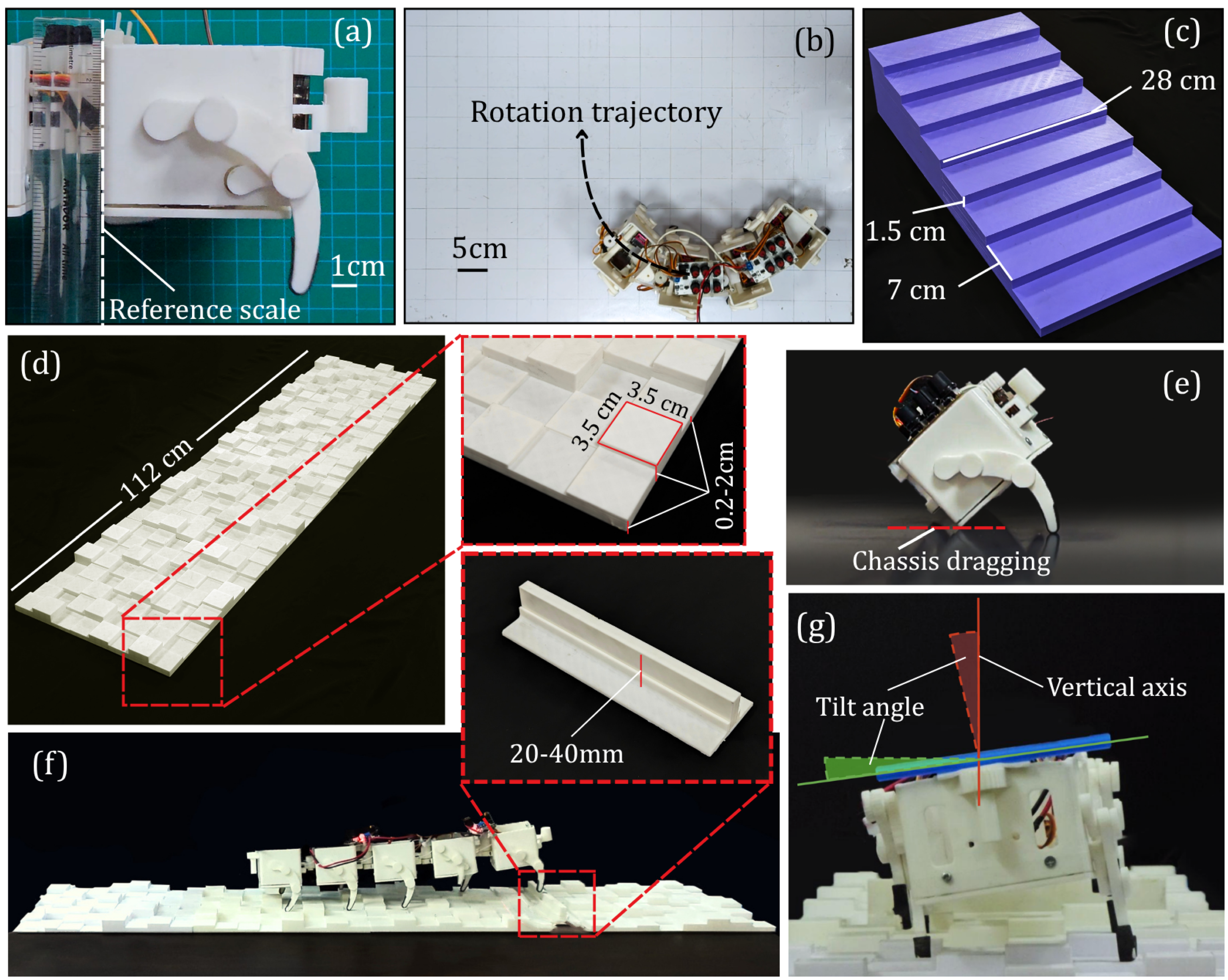
To evaluate the gait of the walking mechanism, a single-module prototype was tested on a flat surface. A 1 cm × 1 cm grid pattern was positioned behind the module’s plane of motion to serve as a fixed spatial reference for coordinate extraction (Figure 3a). The module was actuated for five complete gait cycles, which were recorded using a (3840 × 2160 pixels) camera. To ensure spatial accuracy, the recorded footage was post-processed by scaling the pixel data (background grid) against a physical reference scale fixed to the robot chassis. The extracted experimental trajectories were subsequently compared against simulation results (Figure 1b) to quantitatively evaluate path fidelity and spatial deviation across the locomotion cycle.

2.3.2. Locomotion Performance Evaluation

The locomotion performance of the robotic system was characterized across three distinct environments: flat terrain, stochastic rough terrain, and a custom stair-climbing testbed (Figure 3). Experimental trials were conducted with configurations ranging from two to six modules across all terrains. A single-module configuration was evaluated exclusively on flat terrain, as its inherent design results in chassis-dragging that precludes traversal over irregular or elevated geometries (Figure 3f).
To quantify performance, traversal time and instantaneous current draw were recorded for each configuration. Data acquisition was performed via high-resolution (3840 × 2160 pixels) video recording, which captured the robot’s displacement synchronized with the real-time display of the external power supply for subsequent power consumption analysis. To evaluate consistency, five independent trials were executed for each modular configuration in every environmental scenario.
1.
Flat terrain: Experiments were conducted on a finished wooden surface to establish baseline walking velocity and power consumption. Each modular configuration was tested over a predefined 1 m track to characterize the relationship between module count, steady-state velocity, and electrical load.
2.
Rough terrain: To evaluate locomotion robustness on irregular surfaces, a randomized rough terrain was developed (Figure 3d). The environment comprised four sequentially aligned blocks (280 mm × 280 mm each), forming a 1.12 m track. Each block featured an 8 × 8 grid of cells with stochastic heights ranging from 2 mm to 20 mm ( 4.4 % to 44 % of the robot’s leg length). Traversal over height variations was governed by passive mechanical adaptation rather than active sensing: when the stance leg contacts a taller surface feature, the increased ground reaction force momentarily reduces that leg’s effective speed, redistributing torque to the unloaded swing leg via the shared motor shaft. This self-correcting mechanism allowed each module to independently conform to the stochastic surface profile under open-loop control, without requiring inter-module synchronization.
3.
Stairs: A custom stair assembly was constructed to verify the robot’s capacity to navigate inclined, stepped environments. The apparatus featured eight consecutive steps with a 70 mm tread depth and a 15 mm riser height ( 33 % of the leg length) (Figure 3c).

2.3.3. Robot Maneuverability Evaluation

To characterize the turning performance across different configurations, experimental trials were conducted on a low-friction surface marked with a 50 × 50 mm reference grid (Figure 3b). Based on the geometric constraints identified during the design phase, the maximum joint articulation angle was established as α = 25° (Section 2.1.2). Accordingly, a constant α = 25° was maintained between all adjacent modules during testing to evaluate the minimum achievable collision-free turning radius.
The capacity to execute a circular trajectory is mechanically governed by the inter-module coupling system, which requires a trailing unit to exert the lateral force necessary to rotate the preceding module (Section 2.1.2). Since this interaction is absent in a single-module configuration, maneuverability analysis was restricted to configurations comprising two or more modules.
Trajectory data were captured using an overhead camera to provide an unobstructed plan view of the locomotion path. The resulting planar coordinates were extracted and fitted to the general equation of a circle, ( x x c ) 2 + ( y y c ) 2 = R 2 , using a least-squares approach [40,41,42]. Finally, the empirical turning radii were compared against the theoretical predictions derived from Equation (11) to validate the analytical kinematic model.

2.3.4. Obstacle Clearance Evaluation

To evaluate the robot’s maximum discrete-obstacle crossing capability under rough-terrain conditions, a new experimental setup was created by integrating a custom rough-terrain track with a variable-height obstacle. The rough-terrain track was the same as that used for evaluating rough-terrain performance, consisting of a 280 × 1120 mm surface populated with 35 × 35 mm rigid sections of randomized heights ranging from 2 to 20 mm. A rigid transverse barrier of adjustable height was then incorporated into the track at a distance of 840 mm from the start position (Figure 3f), with obstacle heights varied from 20 to 50 mm.
Configurations with n = 3 to n = 6 modules were evaluated for obstacle clearance. The n = 1 and n = 2 configurations were excluded because prior experiments showed that they could not locomote reliably on the rough-terrain track (Section 3.2). For each configuration, the obstacle height was increased in 1 mm increments, and the maximum height successfully traversed was recorded as the obstacle-clearance limit. All trials were video-recorded, allowing traversal velocities and velocity variances to be measured. Using the corresponding mean power-consumption data, the energy consumption per unit distance was calculated. These experiments were performed with an on-board power supply consisting of a custom 7.4 V, 5000 mAh lithium-ion battery pack fabricated by connecting two Samsung INR21700-50S cells (Generic, Shenzhen, China) in series as described in Section 2.1.4. As the actuation motors needed a 5 V supply, we used a voltage converter (300 W 20 A Step Down Buck Converter, Generic, Shenzhen, China) to convert the 7.4 V supply to 5 V.

2.3.5. Postural Stability Evaluation

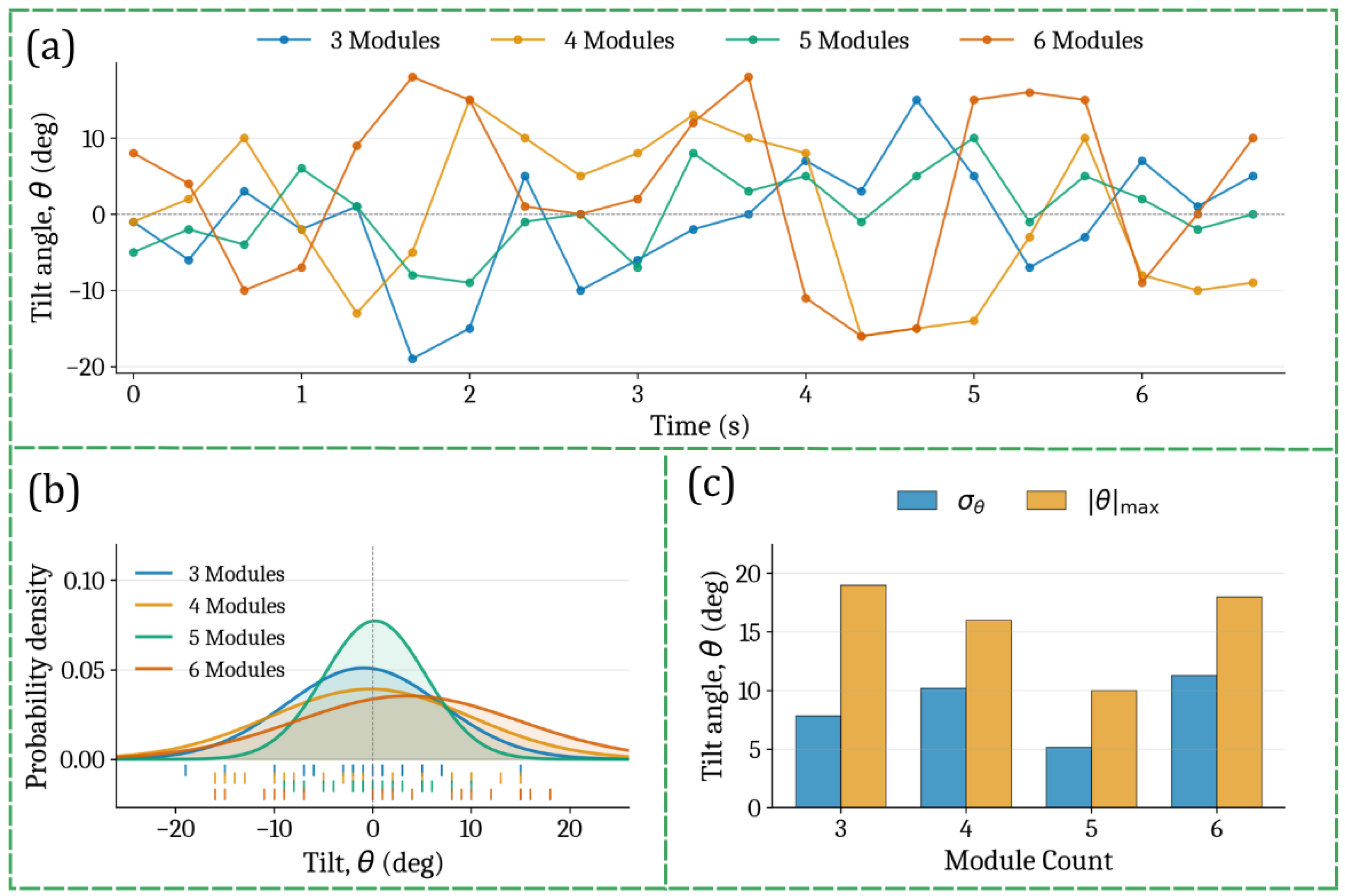
Following [43], the tilt angle θ , defined as the angular deviation of the chassis from the global vertical axis (Figure 3g), was used to quantify locomotion stability. Measurements were obtained during rough-terrain traversal on the custom-designed track (Section 2.3.4, Figure 3f) for configurations with n = 3–6 modules. Video data were captured at a sampling rate of 3 Hz using a camera with an 111 mm equivalent focal length positioned perpendicular to the sagittal plane of the robot. A light-blue marker affixed to the chassis enabled frame-by-frame extraction of θ .
As a balanced bipedal gait is expected to produce oscillations symmetric about the vertical axis [44], the empirical tilt distribution was modeled as a zero-centered Gaussian distribution. The standard deviation σ θ of the fitted distribution was used as the stability metric, with lower σ θ denoting a narrower tilt envelope and superior postural stability. The Shapiro–Wilk test [45] was applied to verify the normality assumption, and inter-configuration differences in dispersion were assessed using the Brown–Forsythe test [46].

2.3.6. Real-World Demonstrations

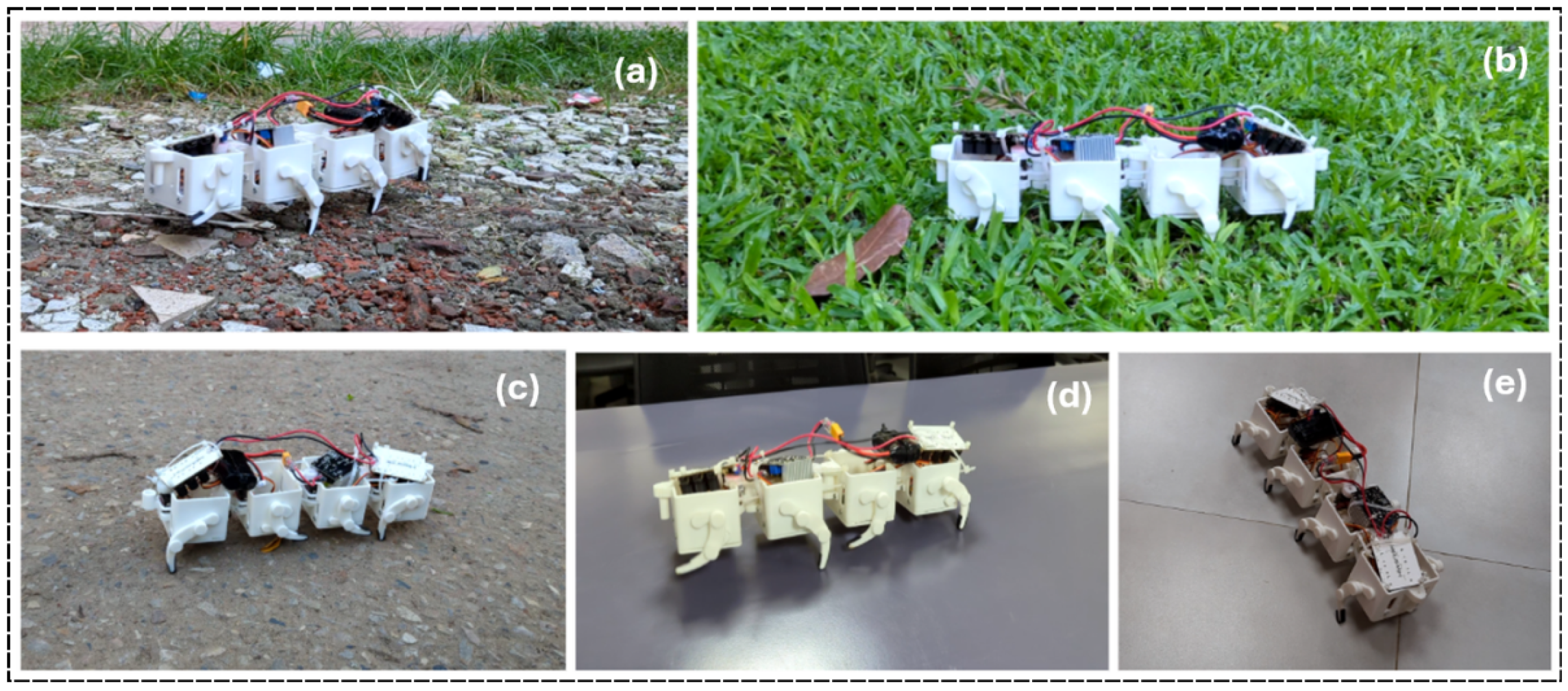
The robot was further tested in unstructured outdoor and indoor environments to verify its practical locomotion capability. Trials were conducted on commonly encountered rough surfaces, including debris-covered ground, grass fields, paved roads, painted wooden tables, and indoor tiles. The four-module configuration was selected for these tests based on its comparatively stable performance in prior experiments.

2.3.7. Cost of Transportation Calculation

The Cost of Transportation (CoT) is an established energy-efficiency metric that quantifies the energy required for transport, normalized by body weight [47,48]. The CoT of Flexipede was derived using the recorded electrical power consumption data from the walking performance valuation experiments, using the following equation:
CoT = P m g v ,
where P is the average electrical power consumption (watts); m is the mass of the robot (kg); g is the gravitational acceleration (9.81 m/s2); and v is the locomotion velocity (m/s). Here, m includes the mass of the onboard battery pack to ensure an accurate representation of the operational payload. A lower CoT value indicates better energy efficiency, meaning the robot travels further for the same energy expenditure per unit weight [47,48,49]. CoT is a particularly useful metric for comparing locomotion efficiency across different module configurations and terrain conditions in a normalized, dimension and mass-independent manner.

2.4. Statistical Analysis

To evaluate the significance of variations of a metric between adjacent module configurations, two-sided, pairwise Mann–Whitney U tests were performed (SciPy v1.13). The null hypothesis assumed identical distributions of the related metric between adjacent configurations. The non-parametric Mann–Whitney U test was selected because it requires no normality assumptions, which is critical given that normality cannot be reliably verified with our sample size of five independent trials per configuration (n = 5). Although tests utilized the same base platform, variations in module count alter the total mass and physical system geometry; configurations were thus treated as independent (unpaired) samples. Given the small sample size (n = 5), the analysis is inherently underpowered for small effect sizes; thus, non-significant outcomes indicate inconclusive trends rather than definitive evidence of no difference. Statistical significance is denoted in all relevant figures using standard brackets: ns ( p 0.05 ), * ( p < 0.05 ), ** ( p < 0.01 ), *** ( p < 0.001 ), and **** ( p < 0.0001 ).

3. Results

3.1. Walking Mechanism Gait

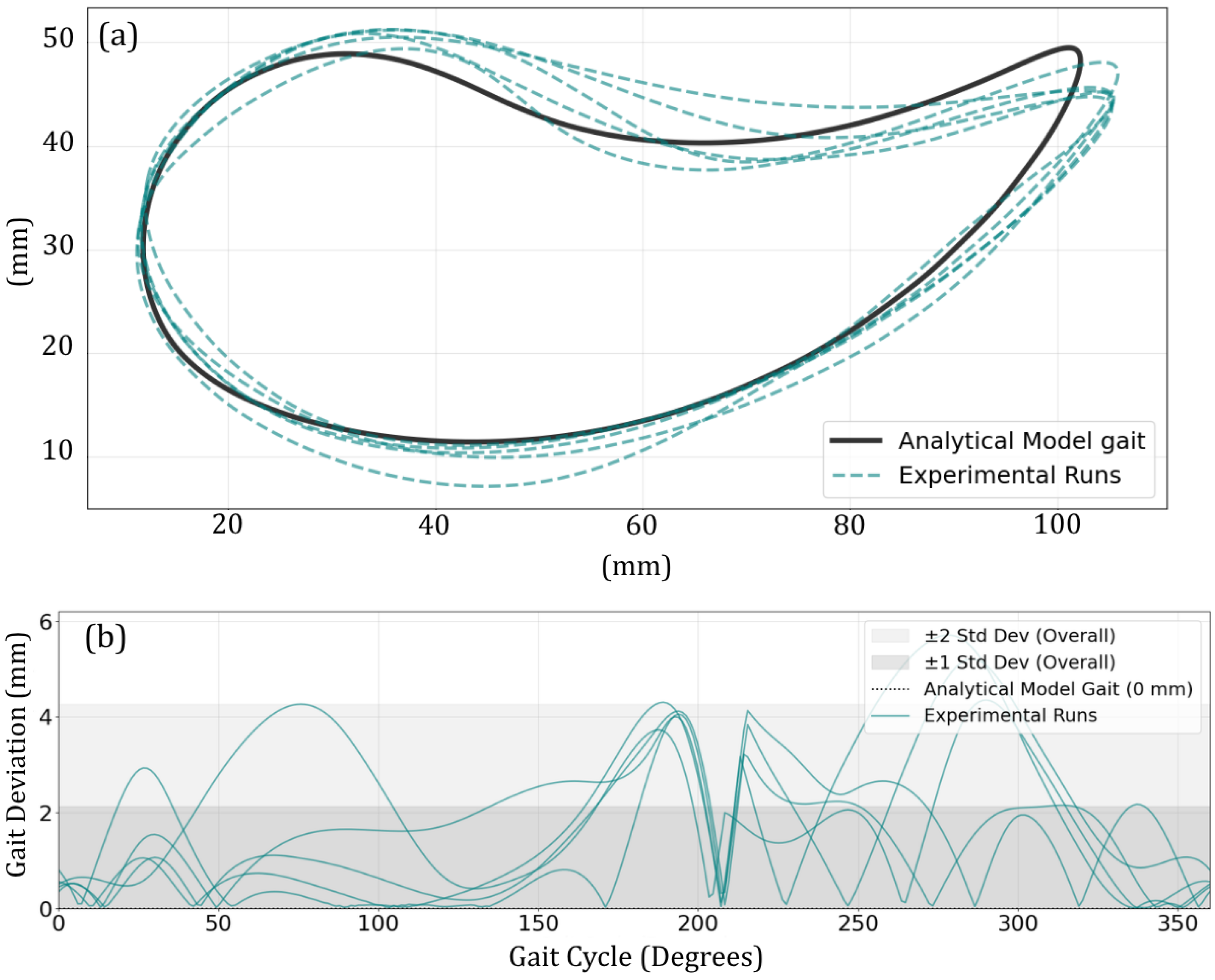
The experimental evaluation of the walking mechanism confirmed a repeatable gait trajectory (Figure 4a). When compared against the analytically derived kinematic model (Section 2.1.1), the physical prototype exhibited a mean vertical deviation of 1.65 mm . Normalizing this value against the Flexipede’s leg length (51 mm) yielded a relative deviation of 3.24 % , demonstrating high path fidelity between the mathematical design and the physical assembly.
Although a peak vertical deviation of 5.71 mm ( 11.20 % ) between the analytical and experimental gait pattern was recorded, the spatial error distribution remained tightly clustered, as illustrated in Figure 4b. Specifically, 68 % ( ± 1 standard deviation) of the sampled trajectory points fell within a margin of 2.13 mm ( 4.18 % ), while 95 % ( ± 2 standard deviation) of the locomotion cycle maintained a deviation below 4.26 mm ( 8.35 % ). These results indicate that the gait remains highly consistent across multiple cycles, with the majority of the path closely adhering to the analytical profile.

3.2. Walking Performance Evaluation

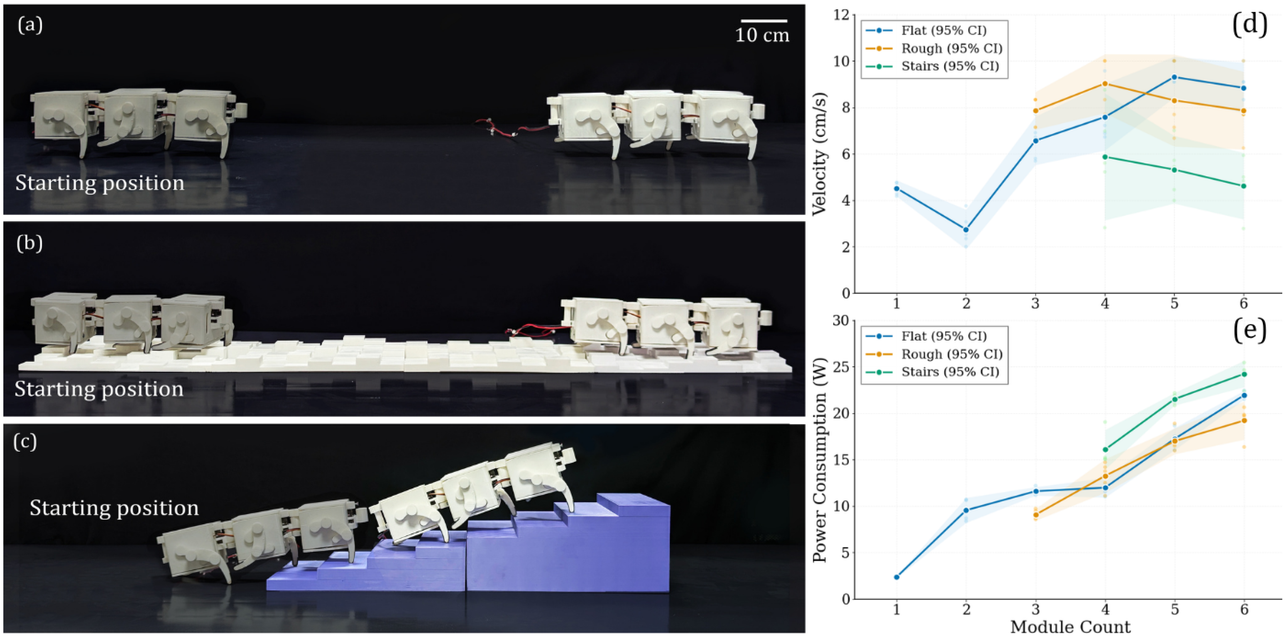
Experimental results revealed Flexipede’s distinct locomotion trends across the three evaluated environments, as illustrated in Figure 5. On flat terrain, velocity exhibited a non-monotonic relationship with module count; speeds initially decreased between the one- and two-module setups before scaling to a peak of 9.30 ± 0.88 cm/s (mean ± 95% CI) for the five-module configuration (Figure 5d).
Navigating irregular geometries required greater mechanical redundancy. Configurations below three modules for rough terrain and four modules for stair climbing failed to progress beyond the initial obstacles, typically becoming immobilized near the starting position.
For rough terrain navigation and stair climbing, peak velocities across all configurations were exhibited by the four-module setup, yielding maximum speeds of 9.02 ± 1.27 cm / s and 5.87 ± 2.73 cm / s , respectively. In these non-level environments, adding modules beyond the four-module mark introduced a performance penalty, with stair-climbing speeds falling to a range of 5.32 to 4.61 cm/s.
System power consumption generally scaled with modularity across all surfaces, with the highest energetic demand observed during stair climbing (Figure 5e). On flat terrain, power draw ranged from 2.28 W to 22.40 W, while rough terrain navigation required between 8.44 W and 21.25 W. The peak system power consumption of 25.63 W was recorded for the six-module configuration during stair ascent, reflecting the substantial torque required to vertically displace the additional mass. These results indicated a consistent energetic penalty associated with increased modularity, particularly during vertical traversal.

3.3. Robot Maneuverability

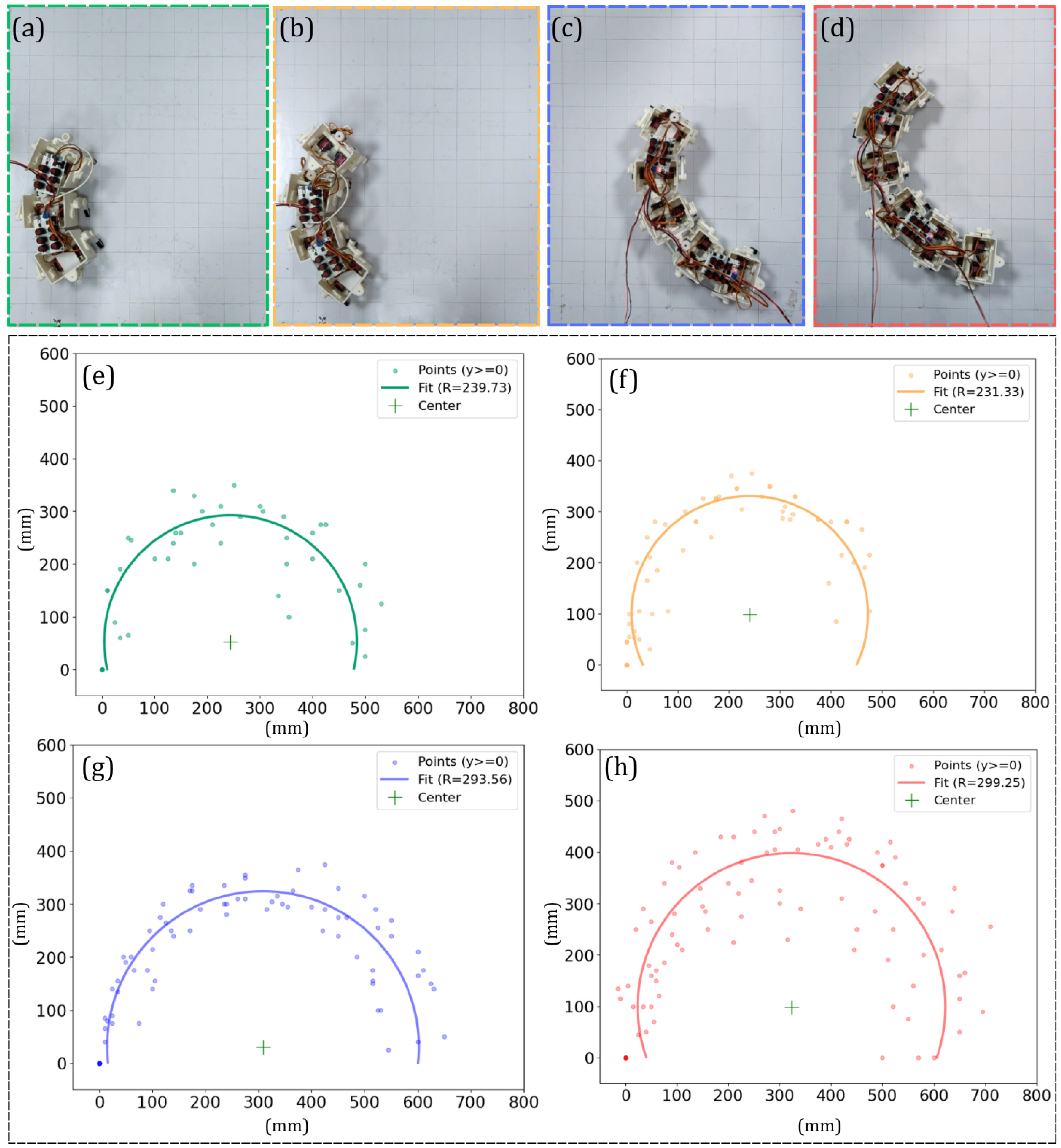
While kinematic modeling predicted a gradual reduction in the turning radius as module count increased, experimental observations revealed a stepped performance trend (Figure 6, Table 3). Notably, the three- and four-module configurations exhibited nearly identical turning radii, a pattern that recurred for the five- and six-module setups. A comparative analysis of empirical measurements and theoretical values showed a percent deviation ranging from 4.51% to 31.49%.
Among all evaluated assemblies, the five-module configuration demonstrated the highest fidelity to the analytical model derived in Section 2.1.2, yielding the minimum observed deviation (4.51%). Conversely, the two-module configuration proved insufficient for executing a complete circular trajectory; the lack of sufficient trailing modules resulted in inadequate lateral force to maintain the required curvature.

3.4. Obstacle Clearing Performance

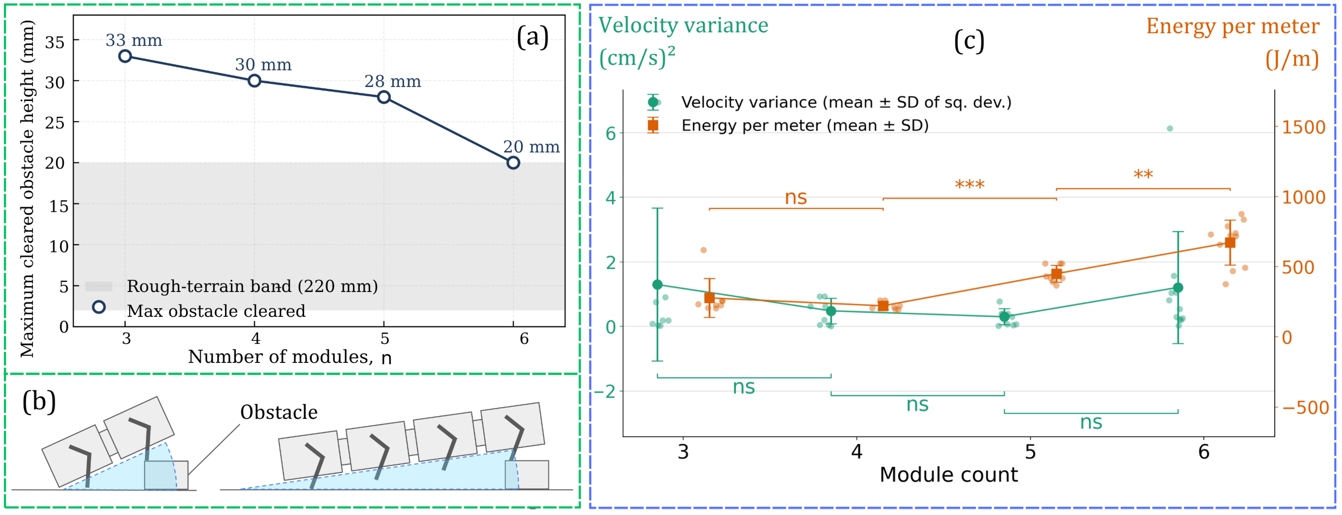
The maximum obstacle-clearance height decreased monotonically with increasing module count, from 33 mm for the three-module configuration to 20 mm for the six-module configuration (Figure 7a). The reduction was approximately linear between n = 3 and n = 5 (approximately 2.3 mm per additional module), followed by a more pronounced decline between n = 5 and n = 6 .
The five-module configuration exhibited the lowest velocity variance, at 0.301 cm / s 2 , indicating the most consistent locomotion performance on rough terrain (Figure 7c). The four-module configuration showed the second-lowest variance (0.484), whereas the three-module and six-module configurations displayed substantially greater variability, with variances of 1.298 cm / s 2 and 1.210 cm / s 2 , respectively. Pairwise Mann–Whitney U tests revealed no statistically significant differences in velocity distributions between configurations with consecutive module counts ( p > 0.05 ).
In terms of transport cost, the four-module configuration was the most energy-efficient, requiring an average of 214.8 J/m (Figure 7c). Although the difference between the three-module and four-module configurations was not statistically significant ( p > 0.05 ), energy consumption increased markedly for configurations with more than four modules.

3.5. Postural Stability

The empirical tilt distributions across all configurations were approximately Gaussian (Shapiro–Wilk p > 0.05 ) and centered near zero ( | μ θ | 3.57 ° ), confirming symmetric chassis oscillations consistent with a balanced gait (Figure 8a,b). The five-module configuration produced the narrowest tilt envelope, with σ θ = 5.17 ° and a 95% confidence interval (CI) of ± 10.33 ° . In contrast, the six-module assembly exhibited the broadest dispersion ( σ θ = 11.30 ° , CI = ± 22.60 ° ), representing a 2.2-fold increase relative to the five-module setup. The three- and four-module configurations occupied intermediate ranges ( σ θ = 7.83 ° to 10.20 ° ). The Brown–Forsythe test confirmed significant heterogeneity in tilt dispersion across configurations ( W = 6.27 , p = 0.0007 ) (Figure 8c), indicating that postural stability did not scale monotonically with modular count.

3.6. Real-World Environments

Field demonstrations validated the functional versatility of the four-module configuration across diverse unstructured environments (Figure 9). The robot successfully navigated both indoor and outdoor terrains, including stochastic debris, soiled grass, paved roads, and tiled flooring. These results confirm that the modular linkage design maintains locomotive stability when transitioning from controlled laboratory settings to the unpredictable friction and topographical variations of real-world deployment.

3.7. Cost of Transportation Analysis

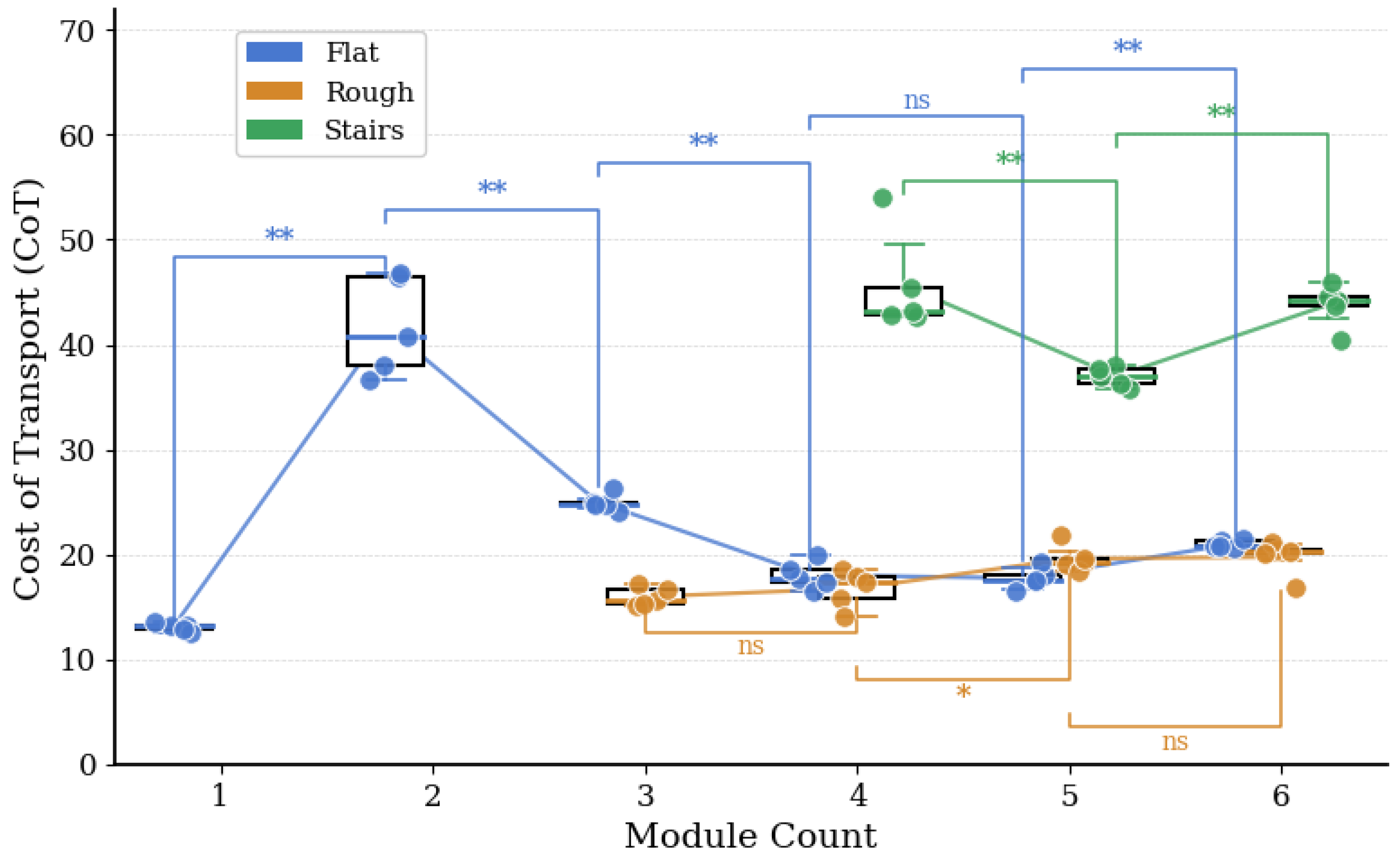
Experimental characterization of the Cost of Transport (CoT) revealed distinct energetic efficiency trends across the evaluated environments (Figure 10). On flat terrain, the CoT peaked at the two-module configuration (mean = 41.74, SD = 4.21 ), representing a statistically significant increase relative to the one-module baseline ( p < 0.01 ). Subsequent increases in module count yielded progressive reductions in CoT, reaching a minimum mean CoT of 17.73 (SD = 1.34 ) for the five-module setup. Subsequently, a small but statistically significant ( p < 0.01 ) uptick in CoT to 21.00 (SD = 0.89 ) was observed for the six-module configuration.
In contrast, CoT values for rough terrain remained relatively stable, exhibiting a gradual increase with higher modular configurations and significantly lower sensitivity to module count (Figure 10). The transition from three to four modules was statistically non-significant ( p 0.05 ), with means of 15.94 (SD = 1.12 ) and 16.02 (SD = 0.87 ), respectively. Subsequently, a modest but statistically significant increase in CoT to 19.20 (SD = 1.43 ) occurred for five-module configurations ( p < 0.05 ). The following transition from five to six modules was non-significant ( p 0.05 ; mean = 20.11 , SD = 1.67 ). For stair climbing, the CoT exhibited highly dynamic scaling across configurations (Figure 10). A statistically significant reduction was observed between the four- and five-module configurations ( p < 0.01 ), with the mean dropping from 43.80 (SD = 4.91 ) to 36.98 (SD = 1.26 ), making five modules the most energetically efficient setup for stair traversal. Conversely, a subsequent and significant increase to 44.13 (SD = 2.08 ) was observed at six modules ( p < 0.01 ). Notably, for all configurations exceeding n = 3 , stair climbing consistently yielded the highest CoT values across all tested environments.

4. Discussion

Experimental results confirmed that the bipedal locomotion mechanism produced a highly repeatable gait, restricting the mean deviation from predicted trajectories to a marginal 3.24 % of the Flexipede’s leg length. With 95% of deviations constrained within an 8.35% threshold, the errors proved functionally negligible, as they neither compromised ground clearance nor disrupted gait continuity. This high degree of correspondence suggests that the linkage system’s structural integrity is sufficient to replicate the intended kinematics, even when using low-cost additive manufacturing. Consequently, the proposed analytical model serves as a reliable predictor of the physical behavior of Flexipede, proving that fabrication tolerances and material compliance do not compromise functional performance. This further demonstrates that the system achieves reliable locomotion without the need for high-precision machining.
The experimental data revealed a non-linear relationship between modular scaling and locomotion performance. While flat-terrain velocity peaked at the five-module configuration, the maximum velocity for complex environments was reached at four modules, suggesting that the parasitic effects of increased mass eventually surpass the added actuator’s torque benefit. Conversely, configurations with fewer than three modules failed to navigate irregular terrains, as their restricted geometric span and reduced ground contact points precluded the mobility required to surmount obstacles. These results underscore that a minimum modular redundancy is essential for Flexipede to provide the mechanical leverage and support polygon necessary to translate drive power into effective locomotion across stochastic geometries.
Analysis of the robot’s performance across diverse surfaces underscored the critical influence of leg-surface interaction on locomotive efficiency. The system exhibited its highest average velocities on rough terrain, outperforming flat-surface speeds by 19 20 % for three- and four-module configurations. This performance gain was attributed to the leg mechanisms intermittently interlocking with surface protuberances, which provided superior traction compared to the flat terrain, where increased slippage inhibited velocity. Conversely, the reduced speeds and elevated power consumption observed during stair traversal reflected a shift in energetic expenditure, as a substantial portion of the input torque was diverted to vertical displacement against gravity.
While the experimental turning radii reflected the underlying kinematic logic, the observed deviations from theoretical models ( 4.51 % to 31.41 % ) highlight the influence of non-ideal physical constraints—such as asymmetric load distribution and stochastic traction loss—that are absent in simplified simulations. Notably, the convergence of physical and predicted behavior improved as modular scaling increased, suggesting that the additional system mass enhanced ground coupling and frictional stability. This increased gravitational loading effectively mitigated intermittent slippage, providing the mechanical grounding necessary to translate drive torque into a predictable rotational arc. This interpretation is supported by the postural-stability results, which showed the lowest tilt-angle variability for the five-module configuration ( σ θ = 5.17 ° ). The subsequent reduction in stability observed for the six-module configuration suggests that the benefits of increased mass saturate beyond five modules, after which inertial penalties begin to dominate. Consistent with this trend, the deviation between the theoretical kinematic turning-radius model and experimental measurements increased again for the six-module configuration ( 13.27 % ), indicating a diminished ability to realize the idealized turning behavior predicted by the kinematic model.
The maximum obstacle-clearance height decreased monotonically with increasing module count, reaching 20   mm for the six-module configuration. At this point, the clearance limit coincided with the upper bound of the ambient terrain roughness, indicating that the robot could only traverse obstacles of height comparable to the surrounding surface features. This trend can be explained with reference to Figure 7b. In configurations with fewer modules, nearly all modules contribute to propulsion and, critically, generate vertical thrust during obstacle negotiation. As the module count increases, however, the intermediate modules become suspended between the leading and trailing modules while crossing an obstacle. These suspended modules contribute little to either forward propulsion or vertical lifting, yet add mass that must be supported by the front and rear modules. The resulting increase in required motor torque reduces the system’s obstacle-climbing capability, leading to progressively lower obstacle-clearance limits as module count increases.
The energetic efficiency of Flexipede was significantly influenced by modular configuration and environmental complexity. The peak Cost of Transport (CoT) observed on flat terrain for the two-module system suggests that low-redundancy configurations suffered from excessive mechanical slip and diminished traction. However, CoT did not vary monotonically with module count. Instead, each terrain exhibited an optimal configuration beyond which energy efficiency deteriorated, with CoT increasing for module counts exceeding four on flat terrain, three on rough terrain, and five on stepped terrain. This trend indicates that the energetic benefits of additional modules eventually become outweighed by the increased mass and associated mechanical losses, leading to diminishing returns in locomotion performance. Because this minimal configuration lacked the geometric span to navigate complex environments, comparative analysis across all terrains was restricted to configurations exceeding three modules. For these higher-module counts, the elevated CoT during stair climbing indicates that the primary energetic penalty transitions from frictional losses on level ground to the high torque requirements of vertical displacement. Notably, the average CoT on rough terrain ( 18.01 ) is comparable to established multipedal platforms like RHex (CoT = 20) [50]—a significant result given that smaller-scale robots typically exhibit reduced scaling efficiencies [47,48,49]. Consequently, this study establishes a benchmark for the energetic efficiency of myriapod-inspired systems that utilize a hybrid actuation strategy combining centralized propulsion and distributed maneuvering.
A comparison with existing modular multi-legged platforms highlighted both the functional strengths and design limitations of Flexipede (Table 4). While comparable systems were generally tested for one or two modular configurations, Flexipede demonstrated stable locomotion across six distinct setups, with the potential for further scalability. Regarding actuation density, the number of actuators per module was among the lowest in its class, comparable to systems by Hoffman et al. [21] and Hou et al. [20], and exceeded only by the single-actuator-based full robot system of Koh et al. [8]. Furthermore, the experimentally measured velocity of Flexipede (4.52–9.30 cm/s) exceeded that of most established modular systems. These results indicate that Flexipede is among the most compact and lightweight designs (0.21 kg base weight with an additional 0.17 kg per module) in the current literature, achieving superior speed-to-mass performance through its minimalist actuation strategy.
While functional, the current version of Flexipede possesses several limitations that warrant future refinement. The current open-loop architecture lacks an active recovery mechanism for cases where multiple legs are simultaneously obstructed; stall detection and corrective maneuvering will require sensor-based closed-loop control. The inter-module coupling mechanism experienced occasional gear slippage, resulting in intermittent decoupling during high-torque trials. Additionally, locomotion on inclined terrains was constrained by the absence of active inter-modular pitch control. Although the linkage parameters successfully generated the target gait, these dimensions have not yet been mathematically optimized for peak efficiency. Finally, the experimental results presented in the current manuscript were obtained using an external power supply to ensure a regulated baseline and to simplify the measurement instrumentation. However, to accurately estimate the real-world energetic performance of Flexipede, these experiments need to be performed using an onboard power supply, which will have implications on performance due to the added weight of the battery, and its internal resistance under high current draw as described in Appendix A. Future iterations will focus on redesigning the modular interface to incorporate active pitch control alongside enhanced yaw control capabilities. Planned refinements to the leg kinematics aim to maximize ground traction and overall locomotive performance. Finally, the integration of onboard odometry and a closed-loop control architecture is expected to significantly enhance system robustness and navigational precision.

5. Conclusions

This paper presents Flexipede, a myriapod-inspired modular robot that demonstrates that robust multi-terrain traversability is attainable through a simple drive system consisting of a single propulsion actuator per module, supplemented by a servo-driven active-yaw steering connector. By shifting complexity to the linkage design, the platform demonstrated that a stable gait can be executed across irregular geometries without high-frequency active sensing. The system was tested across six configurations—the most extensive scaling reported for this architecture—achieving peak velocities of 4.52 9.30 cm/s, which surpassed several existing platforms characterized by higher control overhead.
Experimental results confirmed that the gait mechanism produced highly repeatable trajectories, with functionally negligible deviations between analytical and physical linkage paths (mean deviation of 3.24 % ). While this stability was preserved during modular scaling, performance scaled non-linearly; the four- and five-module setups emerged as the optimal configurations across most of the performance metrics, as the parasitic mass of larger chains eventually exceeded the drive torque capacity. Furthermore, turning radii converged with theoretical predictions as the module count increased—reaching a minimum deviation of 4.51 % for the five-module configuration—suggesting that increased system mass enhanced ground coupling and stabilized the rotational arc. This study also established the first Cost of Transport (CoT) benchmark for a myriapod-inspired platform, yielding an average CoT of 18.01 on rough terrain.
In conclusion, the successful physical validation of Flexipede presented in this paper provides important insights into the physical limits and energetic costs of modular myriapod robotic platforms. The proposed architecture establishes a foundation for a new class of highly adaptable, simplified multi-segmented robots capable of traversing unstructured real-world environments at substantially lower hardware complexity and cost than conventional systems. Although the current open-loop architecture successfully navigates diverse environments, future development will focus on transitioning to a fully autonomous, closed-loop system. Future work will also entail refining the walking gait, increasing inter-module degrees of freedom, integrating distributed feedback sensors, and investigating the impact of modular scaling on gait synchronization. This hardware evolution will lay the groundwork for subsequent adaptation of advanced control strategies, such as adaptive gait modulation and reinforcement learning, to enhance locomotion efficiency.

Author Contributions

Conceptualization, design, and modeling, S.J.S., S.A.D., S.E.A., and A.K.G.; methodology, S.J.S., M.A.C., and S.I.; experimentation, S.J.S., M.A.C., and S.I.; writing—original draft preparation, S.J.S., M.A.C., and S.I.; writing—review and editing, S.A.D., S.E.A., and A.K.G.; supervision, S.A.D., S.E.A., and A.K.G. All authors have read and agreed to the published version of the manuscript.

Funding

This research received no external funding. The article processing charge (APC) was funded by the University of Dhaka.

Institutional Review Board Statement

Not applicable.

Informed Consent Statement

Not applicable.

Data Availability Statement

Data are contained within the article.

Acknowledgments

During the preparation of this manuscript, the authors used ChatGPT (Version GPT-5.5) and Gemini (Version 3.5 Flash) for the purposes of language refinement. The authors have reviewed and edited the output and take full responsibility for the content of this publication.

Conflicts of Interest

The authors declare no conflicts of interest.

Appendix A. Performance with Onboard Power Source

Evaluating the robot’s performance using an onboard power source is essential for accurately characterizing its real-world capabilities. To this end, we conducted a comprehensive evaluation on flat terrain, powering the robot with a custom 7.4 V, 5000 mAh lithium-ion battery pack fabricated by connecting two Samsung INR21700-50S cells in series as described in Section 2.1.4 As the actuation motors are 5 V, we used a voltage converter (300 W 20 A Step Down Buck Converter) to convert the 7.4 V to 5 V. The four-module configuration of Flexipede was used for this experiment. We recorded five independent trials ( n = 5 ) to compare this untethered configuration against our established tethered baseline, which utilized a tethered external regulated DC power supply maintained at 5 V. Consistent with prior evaluations, the experiments were conducted on a finished wooden surface over a predefined 1-m track (Section 2.3.2). Data acquisition was performed using a high-fidelity camera (3840 × 2160 pixels) with a 72 mm equivalent focal length to minimize perspective distortion during velocity calculations, while instantaneous power consumption was concurrently recorded.
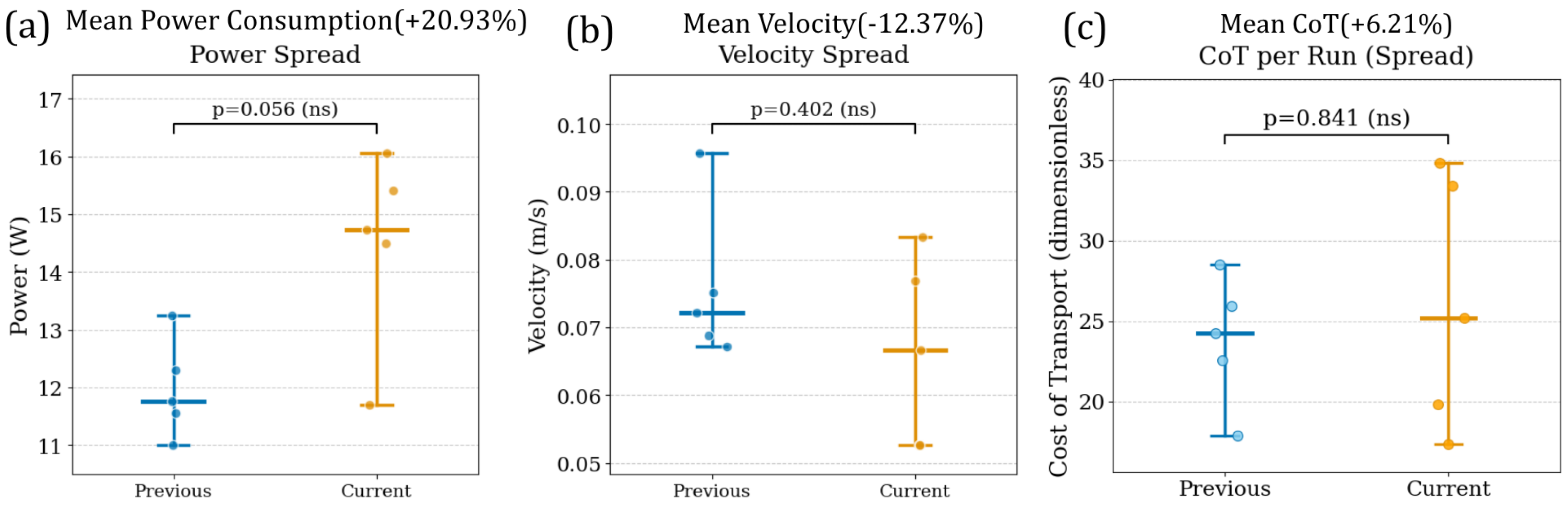
The onboard battery configuration resulted in a 20.93% increase in mean power consumption, a 12.37% decrease in mean velocity, and a 6.21% increase in mean Cost of Transport (CoT) relative to the tethered baseline (Figure A1), arising from the added weight of the battery and the voltage converter. While these differences did not reach strict statistical significance due to the small sample size, the consistent directional trend confirms that the external-supply power measurements represent a conservative lower bound on real-world energy demand. Consequently, the CoT values reported throughout this study represent conservative estimates, with an estimated real-world correction factor of 1.06 for onboard-battery deployment.
Figure A1. (a) Power spread, (b) Velocity spread, and (c) Cost of Transport (CoT) spread between the tethered external supply (Previous) and the onboard battery (Current). The onboard battery configuration resulted in a 20.93% increase in mean power consumption, a 12.37% decrease in mean velocity, and a 6.21% increase in mean CoT. However, the differences between the configurations were not statistically significant (ns) across any of the evaluated metrics (Power: p = 0.056 ; Velocity: p = 0.402 ; CoT: p = 0.841 ).
Robotics 15 00129 g0a1

Appendix B. Maximum Module Count Under the Self-Collision Constraint

The robot is an articulated chain of n rigid modules of length L = 105.688 mm, connected by revolute joints with maximum bend angle α = 25 ° . When every joint is at α , the minimum turning radius of the head is as follows:
R ( n ) = m C + C m 2 + 1 ,
m = cot ( n 1 ) α ,
C = L + k = 1 n 2 L cos ( k α ) cot ( n 1 ) α k = 1 n 2 L sin ( k α ) .
This derivation assumes a single C-shaped arc, valid while ( n 1 ) α < 180 ° ; outside this range, the cotangent is singular and rows with R ( n ) 0 are excluded (flagged singular in Table A1). At the minimum-radius pose, the chain body is tangent to the incircle of radius R ( n ) , and the no-collision condition reduces to a circumscribed polygon constraint. For a regular polygon with apothem R and side L, the maximum admissible module count is
n max ( R ) = π arctan L / ( 2 R ) ,
and the constraint is n n max ( R ( n ) ) . Table A1 evaluates this for n = 2 , , 22 , with the slack Δ ( n ) n max ( R ( n ) ) n . The slack changes sign between n = 18 ( Δ = + 1.27 ) and n = 19 ( Δ = 1.50 ), giving:
n = 18 .
The admissible result n = 18 lies in the second algebraic branch ( ( n 1 ) α = 425 ° , wrapping once around the turning centre); restricting to the principal branch ( n 1 ) α < 180 ° yields n = 8 as the single-arc limit.
Table A1. Minimum trajectory radius and circumscribed-polygon capacity for α = 25, L = 105.688 mm. Admissibility is decided by the sign of Δ = n max ( R ( n ) ) n where R ( n ) > 0 .
n ( n 1 ) α []mC [ mm ]R [ mm ] n max Δ Status
225.002.1445105.69476.7328.46 + 26.46 admissible
350.000.8391164.00351.6921.06 + 18.06 admissible
475.000.2679235.75307.2318.44 + 14.44 admissible
5100.00−0.1763336.92282.7117.00 + 12.00 admissible
6125.00−0.7002510.74265.8716.01 + 10.01 admissible
7150.00−1.7321942.43252.5215.23 + 8.23 admissible
8175.00−11.43015512.27240.6714.54 + 6.54 admissible
16375.003.732184.23639.7538.12 + 22.12 admissible
17400.001.1918139.60383.5522.95 + 5.95 admissible
18425.000.4663204.70321.3119.27+1.27admissible
19450.000.0000291.21291.2117.50−1.50self-collision
20475.00−0.4663427.00272.0316.37−3.63self-collision
21500.00−1.1918707.74257.6015.53−5.47self-collision
22525.00−3.73211863.40245.3214.81−7.19self-collision

References

  1. Williams, A.; Sebastian, B.; Ben-Tzvi, P. Review and analysis of search, extraction, evacuation, and medical field treatment robots. J. Intell. Robot. Syst. 2019, 96, 401–418. [Google Scholar] [CrossRef]
  2. Cai, Z. RescueFlex: A modular intelligent rescue robot system for complex disaster scenarios. In AHFE International; AHFE International: Orlando, FL, USA, 2025; Volume 195. [Google Scholar]
  3. Torige, A.; Noguchi, M.; Ishizawa, N. Centipede type multi-legged walking robot. In Proceedings of 1993 IEEE/RSJ International Conference on Intelligent Robots and Systems (IROS’93); IEEE: Yokohama, Japan, 26–30 July 1993; Volume 1, pp. 567–571. [Google Scholar]
  4. Zhang, Y.; Arakelian, V. Design and synthesis of single-actuator walking robots via coupling of linkages. Front. Mech. Eng. 2021, 6, 609340. [Google Scholar] [CrossRef]
  5. Sherry, F.; Zhou, C. Design of a Transforming Myriapod Robot for Multimodal Locomotion. In UKRAS21 Conference: Robotics at home Proceedings; EPSRC UK Robotics and Autonomous Systems (RAS) Network: London, UK, 2021. [Google Scholar]
  6. McClure, J.; Sahin, F. A low-cost search-and-rescue drone for near real-time detection of missing persons. In 2019 14th Annual Conference System of Systems Engineering (SoSE); IEEE: Piscataway, NJ, USA, 2019; pp. 13–18. [Google Scholar]
  7. Apvrille, L.; Tanzi, T.; Dugelay, J.-L. Autonomous drones for assisting rescue services within the context of natural disasters. In 2014 XXXIth URSI General Assembly and Scientific Symposium (URSI GASS); IEEE: Piscataway, NJ, USA, 2014; pp. 1–4. [Google Scholar]
  8. Koh, D.; Yang, J.; Kim, S. Centipede robot for uneven terrain exploration: Design and experiment of the flexible biomimetic robot mechanism. In 2010 3rd IEEE RAS & EMBS International Conference on Biomedical Robotics and Biomechatronics; IEEE: Piscataway, NJ, USA, 2010; pp. 877–881. [Google Scholar]
  9. van Marum, B.; Sabatelli, M.; Kasaei, H. Learning perceptive bipedal locomotion over irregular terrain. arXiv 2023, arXiv:2304.07236. [Google Scholar]
  10. Badri-Spröwitz, A.; Sarvestani, A.A.; Sitti, M.; Daley, M.A. BirdBot achieves energy-efficient gait with minimal control using avian-inspired leg clutching. Sci. Robot. 2022, 7, eabg4055. [Google Scholar] [PubMed]
  11. Kyle, J.; Yim, J.K.; Hart, K.; Bergbreiter, S.; Johnson, A.M. The Simplest Walking Robot: A bipedal robot with one actuator and two rigid bodies. In 2023 IEEE-RAS 22nd International Conference on Humanoid Robots (Humanoids); IEEE: Piscataway, NJ, USA, 2023; pp. 1–7. [Google Scholar]
  12. Ottaviano, E.; Grande, S.; Ceccarelli, M. A biped walking mechanism for a rickshaw robot. Mech. Based Des. Struct. Mach. 2010, 38, 227–242. [Google Scholar] [CrossRef]
  13. Man, S.; Narita, S.; Macera, J.; Oke, N.; Johnson, A.M.; Bergbreiter, S. Zippy: The smallest power-autonomous bipedal robot. arXiv 2025, arXiv:2505.05686. [Google Scholar]
  14. Collins, S.H.; Ruina, A. A bipedal walking robot with efficient and human-like gait. In Proceedings of the 2005 IEEE International Conference on Robotics and Automation; IEEE: Piscataway, NJ, USA, 2005; pp. 1983–1988. [Google Scholar]
  15. Aoi, S.; Yabuuchi, Y.; Morozumi, D.; Okamoto, K.; Adachi, M.; Senda, K.; Tsuchiya, K. Maneuverable and efficient locomotion of a myriapod robot with variable body-axis flexibility via instability and bifurcation. Soft Robot. 2023, 10, 1028–1040. [Google Scholar] [CrossRef] [PubMed]
  16. Chong, B.; Wang, Y.; Kan, J.H.; Karsai, G.; Sato, D.D.; Blekherman, G.; Goldman, D.I. Multilegged matter transport: A framework for locomotion on noisy landscapes. Science 2023, 380, 509–515. [Google Scholar] [CrossRef] [PubMed]
  17. Yasui, K.; Takano, S.; Kano, T.; Ishiguro, A. Adaptive centipede walking via synergetic coupling between decentralized control and flexible body dynamics. Front. Robot. AI 2022, 9, 797566. [Google Scholar] [CrossRef] [PubMed]
  18. Yin, H.; Shi, R.; Liu, J. Structural Design and Control Research of Multi-Segmented Biomimetic Millipede Robot. Biomimetics 2024, 9, 288. [Google Scholar] [CrossRef] [PubMed]
  19. Ozkan-Aydin, Y.; Chong, B.; Aydin, E.; Goldman, D.I. A systematic approach to creating terrain-capable hybrid soft/hard myriapod robots. In 2020 3rd IEEE International Conference on Soft Robotics (RoboSoft); IEEE: Piscataway, NJ, USA, 2020; pp. 156–163. [Google Scholar]
  20. Hou, J.; Xue, Z.; Liang, Y.; Sun, Y.; Zhao, Y.; Chen, Q. Self-configurable centipede-inspired rescue robot. Appl. Sci. 2024, 14, 2331. [Google Scholar]
  21. Hoffman, K.L.; Wood, R.J. Myriapod-like ambulation of a segmented microrobot. Auton. Robot. 2011, 31, 103–114. [Google Scholar] [CrossRef]
  22. Ackerman, E. Giant Robotic Bugs Are Headed to Farms. IEEE Spectrum. 2025. Available online: https://spectrum.ieee.org/ground-control-robot-insects (accessed on 1 May 2026).
  23. Bulichev, O.; Klimchik, A. Concept Development Of Biomimetic Centipede Robot StriRus. In 2018 23rd Conference of Open Innovations Association (FRUCT); IEEE: Piscataway, NJ, USA, 2018; pp. 85–90. [Google Scholar]
  24. Ito, K.; Ishigaki, Y. Semiautonomous centipede-like robot for rubble–development of an actual scale robot for rescue operation. Int. J. Adv. Mechatron. Syst. 2015, 6, 177–186. [Google Scholar]
  25. Hayakawa, T.; Kamimura, T.; Kaji, S.; Matsuno, F. Autonomous distributed system for gait generation for single-legged modular robots connected in various configurations. IEEE Trans. Robot. 2020, 36, 1491–1510. [Google Scholar] [CrossRef]
  26. Ahmadzadeh, H.; Masehian, E.; Asadpour, M. Modular robotic systems: Characteristics and applications. J. Intell. Robot. Syst. 2016, 81, 317–357. [Google Scholar]
  27. Baca, J.; Hossain, S.; Dasgupta, P.; Nelson, C.A.; Dutta, A. Modred: Hardware design and reconfiguration planning for a high dexterity modular self-reconfigurable robot for extra-terrestrial exploration. Robot. Auton. Syst. 2014, 62, 1002–1015. [Google Scholar] [CrossRef]
  28. Altendorfer, R.; Saranli, U.; Komsuoglu, H.; Koditschek, D.E.; Komsuoglu, H.; Buehler, M.; Rizzi, N.; Quinn, A.J.; Full, R.J. RHex: A biologically inspired hexapod runner. Auton. Robot. 2001, 11, 207–213. [Google Scholar] [CrossRef]
  29. Subramaniam, S.R.; Samykano, M.; Selvamani, S.K.; Ngui, W.K.; Kadirgama, K.; Sudhakar, K.; Idris, M.S. 3D printing: Overview of PLA progress. In AIP Conference Proceedings; AIP Publishing LLC: Melville, NY, USA, 2019; Volume 2059, p. 020015. [Google Scholar]
  30. Tümer, E.H.; Erbil, H.Y. Extrusion-based 3D printing applications of PLA composites: A review. Coatings 2021, 11, 390. [Google Scholar] [CrossRef]
  31. Lovasz, E.C.; Pop, C.; Pop, F.; Dolga, V. Novel solution for leg motion with 5-link belt mechanism. Int. J. Appl. Mech. Eng. 2014, 19, 699–708. [Google Scholar] [CrossRef]
  32. Martínez-García, E.A.; Domínguez, J.; Lavrenov, R. Dynamic modelling and control of an underactuated Klann-based hexapod. In 2019 12th International Conference on Developments in eSystems Engineering (DeSE); IEEE: Piscataway, NJ, USA, 2019; pp. 64–69. [Google Scholar]
  33. Li, T.; Ceccarelli, M. Design and simulated characteristics of a new biped mechanism. Robotica 2015, 33, 1568–1588. [Google Scholar]
  34. Haldane, D.W.; Fearing, R.S. Running beyond the bio-inspired regime. In 2015 IEEE International Conference on Robotics and Automation (ICRA); IEEE: Piscataway, NJ, USA, 2015; pp. 4539–4546. [Google Scholar]
  35. Telengre, H.S.; Dike, P.; Bandu, S.T.; Jadhav, V.R. A Study on Robotics Arm Vehicle using ESp32 and PS3 controller. Int. J. Sci. Innov. Eng. 2025, 2, 500–504. [Google Scholar]
  36. OrcaSlicer. OrcaSlicer: Open-Source Slicer for FDM Printers. 2024. Available online: https://orca-slicer.com/ (accessed on 8 April 2026).
  37. Kafle, A.; Luis, E.; Silwal, R.; Pan, H.M.; Shrestha, P.L.; Bastola, A.K. 3D/4D printing of polymers: Fused Deposition Modelling (FDM), Selective Laser Sintering (SLS), and Stereolithography (SLA). Polymers 2021, 13, 3101. [Google Scholar] [CrossRef] [PubMed]
  38. Pandzic, A.; Hodzic, D.; Hajro, I.; Tasic, P. Strength properties of PLA material obtained by different models of FDM 3D printer. In Proceedings of the 31st DAAAM International Symposium on Intelligent Manufacturing and Automation, Mostar, Bosnia and Herzegovina, 21–24 October 2020; pp. 1726–9679. [Google Scholar]
  39. Zhao, Y.; Chen, Y.; Zhou, Y. Novel mechanical models of tensile strength and elastic property of FDM AM PLA materials: Experimental and theoretical analyses. Mater. Des. 2019, 181, 108089. [Google Scholar] [CrossRef]
  40. Chernov, N. Circular and Linear Regression: Fitting Circles and Lines by Least Squares; Chapman & Hall/CRC: Boca Raton, FL, USA, 2010. [Google Scholar]
  41. Gander, W.; Golub, G.H.; Strebel, R. Least-squares fitting of circles and ellipses. BIT Numer. Math. 1994, 34, 558–578. [Google Scholar] [CrossRef]
  42. Coope, I.D. Circle fitting by linear and nonlinear least squares. J. Optim. Theory Appl. 1993, 76, 381–388. [Google Scholar] [CrossRef]
  43. Liu, J.; Liu, J.; Xue, Z.; Wu, Y. Research on stability of modular multi-legged robots with non-isomorphic configurations. Trans. Inst. Meas. Control. 2024, 48, 122–134. [Google Scholar] [CrossRef]
  44. Chen, C.; Guo, W.; Wang, P.; Sun, L.; Zha, F.; Shi, J.; Li, M. Attitude trajectory optimization to ensure balance hexapod locomotion. Sensors 2020, 20, 6295. [Google Scholar] [CrossRef] [PubMed]
  45. Shapiro, S.S.; Wilk, M.B. An analysis of variance test for normality (complete samples). Biometrika 1965, 52, 591–611. [Google Scholar] [CrossRef]
  46. Brown, M.B.; Forsythe, A.B. Robust tests for the equality of variances. J. Am. Stat. Assoc. 1974, 69, 364–367. [Google Scholar] [CrossRef]
  47. Seok, S.; Wang, A.; Chuah, M.Y.; Hyun, D.J.; Lee, J.; Otten, D.M.; Lang, J.H.; Kim, S. Design principles for energy-efficient legged locomotion and implementation on the MIT Cheetah robot. IEEE/ASME Trans. Mechatron. 2015, 20, 1117–1129. [Google Scholar]
  48. Coe, M.; Gutschmidt, S. Cost of transport is not the whole story— A review. Ocean. Eng. 2024, 313, 119332. [Google Scholar] [CrossRef]
  49. Luneckas, M.; Luneckas, T.; Kriaučiūnas, J.; Udris, D.; Plonis, D.; Damaševičius, R.; Maskeliūnas, R. Hexapod robot gait switching for energy consumption and cost of transport management using heuristic algorithms. Appl. Sci. 2021, 11, 1339. [Google Scholar] [CrossRef]
  50. Birkmeyer, P.; Peterson, K.; Fearing, R.S. DASH: A dynamic 16g hexapedal robot. In 2009 IEEE/RSJ International Conference on Intelligent Robots and Systems; IEEE: Piscataway, NJ, USA, 2009; pp. 2683–2689. [Google Scholar]
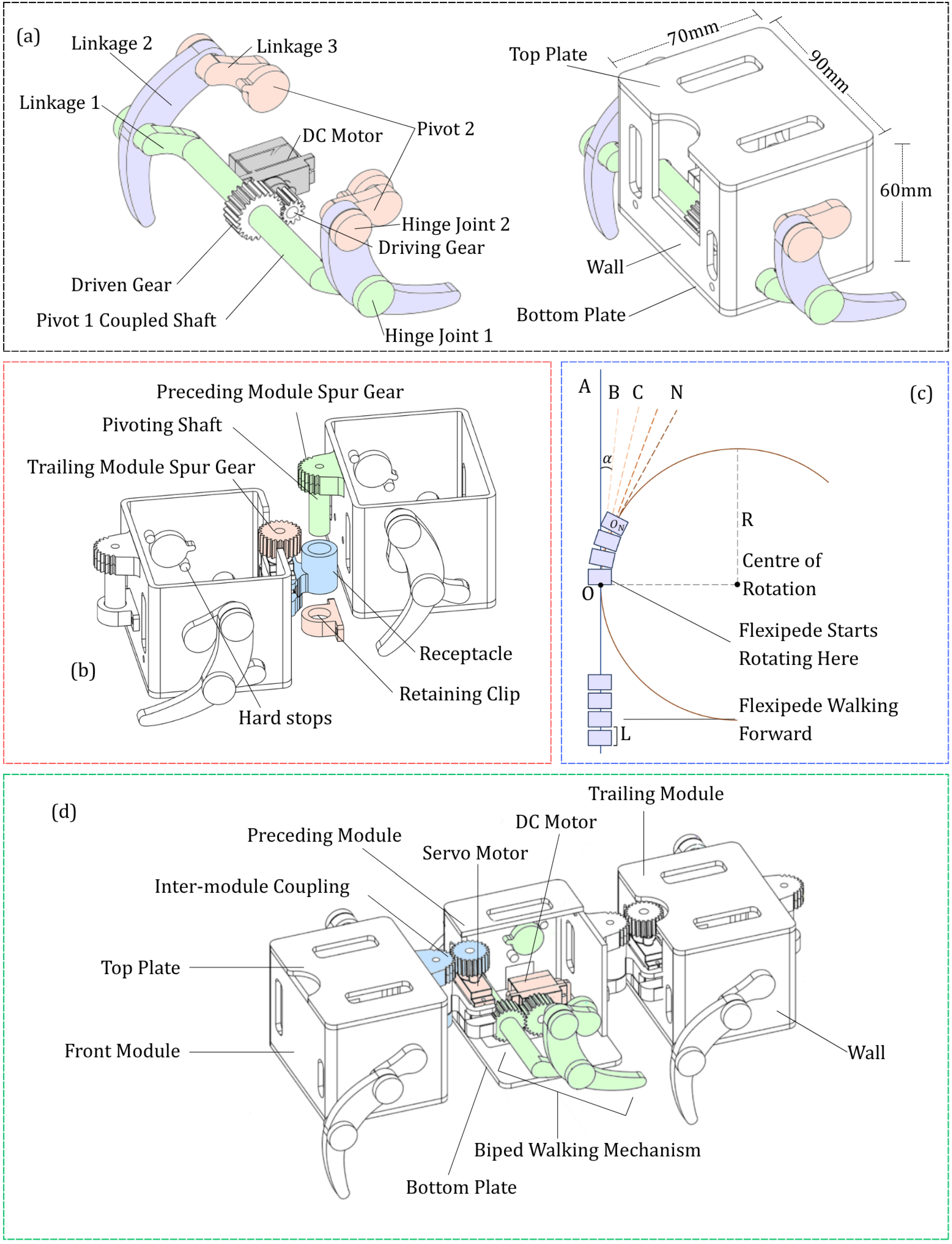
Figure 2. Computer-aided design (CAD) and geometric modeling of Flexipede’s modular assembly. (a) Bipedal walking mechanism derived from the 4-bar linkage parameters specified in Table 1. The assembly was mirrored with a 180° phase shift for L 1 and integrated with a gear train to transmit rotational motion from a single DC motor to the primary shaft at P i v o t 1 . The custom enclosure features removable plates for internal access. (b) Inter-module coupling of two Flexipede units, illustrating the servo-driven articulation of the preceding module relative to the trailing unit. (c) A geometric model to predict the turning radii for varied modular configurations. (d) Three-module Flexipede assembly, featuring an internal view of the central module to detail the spatial integration of the walking and coupling mechanisms.
Robotics 15 00129 g002
Figure 3. Experimental setup and procedures for robotic performance characterization. (a) Close-up view of the leg mechanism aligned with a reference scale for kinematic gait evaluation. (b) Top-down trajectory analysis of the modular assembly during circular maneuverability trials. (c) Custom stair-climbing testbed featuring standardized step geometries for vertical mobility assessment. (d) Rough terrain track comprising four sequentially aligned square blocks ( 280 × 280 mm each), forming a combined 1.12 m track. Each block was subdivided into an 8 × 8 grid of cells ( 35 × 35 mm per cell), with each cell assigned a stochastic height drawn from a uniform distribution ranging from 2 mm to 20 mm ( 4.4 % to 44 % of the robot’s leg length). A zoomed inset highlights the block cell geometry and representative height variation. (e) Single-module configuration illustrating the physical limitations of minimal scaling, specifically chassis-dragging resulting from insufficient ground clearance. (f) Obstacle clearance evaluation setup consisting of the custom uneven terrain track ( 280 × 1120 mm) with a rigid transverse barrier of adjustable height (20–50 mm) placed at 820 mm from the start of the bed. (g) Experimental setup demonstrating θ evaluation process for Postural Stability Evaluation on rough terrain.
Robotics 15 00129 g003
Figure 4. Kinematic validation and repeatability analysis of the gait mechanism. (a) Comparison between the analytically derived and the experimentally measured gait paths of the distal tip of the Flexipede’s leg. (b) Deviation analysis of the experimental gait over a complete 360 ° locomotion cycle. The teal trace represents the point-wise gait deviation from the analytical model, while the shaded regions indicate the ± 1 standard deviation and ± 2 standard deviation bands.
Robotics 15 00129 g004
Figure 5. Locomotion performance and energetic analysis of Flexipede across diverse environments. (ac) Time-lapse illustrations of the robot traversing: (a) flat terrain, (b) stochastic rough terrain, and (c) the custom stair-climbing testbed. (d) Locomotion velocity as a function of module count across all terrain types. (e) Comparative power consumption analysis illustrating the relationship between modularity and environmental resistance. In both (d,e), data points represent the mean of five independent trials, and the shaded regions denote the 95% confidence interval.
Robotics 15 00129 g005
Figure 6. Experimental characterization of turning performance for multi-module configurations. (ad) Representative snapshots of the circular maneuverability trials for the: (a) three-module, (b) four-module, (c) five-module, and (d) six-module configurations. (eh) Corresponding trajectory analysis and geometric circle fitting for the: (e) three-module, (f) four-module, (g) five-module, and (h) six-module setups. Planar coordinates were extracted from plan-view footage and fitted to the general equation of a circle using a least-squares approach to determine the empirical turning radius.
Robotics 15 00129 g006
Figure 7. Obstacle clearance performance analysis. (a) Maximum cleared obstacle height as a function of module count n (3 to 6). The monotonic decline in clearance ceiling converges toward the upper bound of the rough-terrain band (20 mm) at n = 6 , indicating the practical obstacle-negotiation limit of the system. (b) Schematic illustration of the obstacle-clearance geometry with 2-module configuration and 4-module configuration. (c) Velocity variance and energy consumption per unit distance across modular configurations (n = 3–6) during rough terrain obstacle clearance. Energy per unit distance (mean power × traversal time) is presented as mean ± standard deviation. Pairwise differences between adjacent configurations were evaluated using the two-sided Mann-Whitney U test. ns ( p 0.05 ), ** ( p < 0.01 ), *** ( p < 0.001 ).
Robotics 15 00129 g007
Figure 8. Postural stability characterization of Flexipede on stochastic rough terrain in terms of tilt angle ( θ ). (a) Trajectories of θ ( t ) for modular configurations of n = 3 to 6 over a 6.7 s observation window. (b) Gaussian fits of the empirical tilt distributions (Shapiro–Wilk p = 0.689 , 0.092 , 0.884 , and 0.084 for n = 3 to 6, respectively; all p > 0.05 , confirming normality); vertical rug marks denote individual angular samples. (c) Standard deviation of tilt angle ( σ θ = 7.83 ° , 10.20 ° , 5.17 ° , and 11.30 ° for n = 3 to 6, respectively) and maximum absolute tilt ( | θ | max = 19 ° , 16 ° , 10 ° , and 18 ° ) as a function of module count, with lower values indicating tighter tilt envelopes and superior stability. Tilt magnitude differed significantly across configurations (Kruskal–Wallis on | θ | : H = 16.99 , p < 0.001 ; Brown–Forsythe: W = 6.27 , p < 0.001 ).
Robotics 15 00129 g008
Figure 9. Real-world deployment of the four-module Flexipede configuration. (ae) Field demonstrations across diverse unstructured and structured environments: (a) stochastic debris, (b) soiled grass, (c) paved roadway, (d) finished wooden substrate, and (e) indoor tiled flooring. The four-module assembly was selected for these trials as it demonstrated the optimal balance of velocity and energetic efficiency in laboratory characterization.
Robotics 15 00129 g009
Figure 10. Cost of Transport (CoT) across modular configurations ( n = 1 to 6) and terrain types (Flat, Rough, Stairs). CoT was derived from experimental power consumption and velocity data across all environmental conditions. For each terrain–module combination, five independent trials were conducted; scatter points represent individual trial measurements and solid lines connect the mean CoT values across module configurations. Overlaid box plots display the median and interquartile range (IQR) for each configuration. Significance brackets indicate two-sided pairwise Mann–Whitney U test results between adjacent configurations within each terrain: ns ( p 0.05 ), * ( p < 0.05 ), ** ( p < 0.01 ). These metrics illustrate energetic efficiency boundaries and statistical trends as a function of system modularity.
Robotics 15 00129 g010
Table 1. Kinematic design parameters and optimization search space for the walking mechanism. These design parameters were determined through a custom kinematic simulation based on loop-closure Equations (1) and (2) implemented through Python (v3.12) Matplotlib library (v3.10.3). The optimization utilized the defined search space to ensure a continuous walking gait and a closed-loop distal endpoint trajectory.
ParameterSearch SpaceSelected Value
L 1 10–60 mm19.5 mm
L 2 10–60 mm35.5 mm
L 2 e x t 10–60 mm51 mm
L 0 X 10–60 mm27.5 mm
L 0 Y 10–60 mm22.5 mm
L 3 10–60 mm20 mm
L 2 e x t to L 2 offset angle20–60 degrees40 degrees
Table 2. Cost of Flexipede components for a primary module. The unit cost for a fully integrated primary module, including the control system and power source, was $58. Each additional module, comprising only the mechanical chassis, drive linkages, and actuation system, incurred an incremental cost of $10.
ElementModel NameQtyTotal Cost
MotorsMG90S Servo1$7.00
BatterySamsung INR21700-50S 2222$40.94
MicrocontrollerESP32-C3 Super Mini1$4.90
Circuitry (PCB)Custom Integrated1$2.16
StructurePLA+ (102gm)1$1.67
MiscellaneousScrews and Glue$1.33
Total Parts Cost (Initial Module)$58.00
Table 3. Quantitative comparison of theoretical and measured turning radii across modular configurations. The relative deviation (%) is calculated as |Theoretical radius − Measured radius|/Theoretical radius × 100%, where theoretical values are derived from the kinematic model established in Equation (11).
Module Count, nTheoretical Radius (cm)Measured Radius (cm)Relative Deviation (%)
334.9423.9431.49
430.5323.1324.23
528.0929.364.51
626.4229.9313.27
Table 4. Comparison of the Flexipede platform with existing modular multi-legged robotic systems reported in the literature.
RobotModule CountLeg Count per ModuleActuator per ModuleVelocity (cm/s)Dimension per Module (cm)Mass (kg)
Aoi’s Myriapod [15]624/5-135 (l) (full robot)9.1
Torige’s centipede robot [3]5–6240.8627 (w), 20 (l), 15 (h)-
KARASAKA [25]6–71336 (r)0.7 per module
Ozkan-aydin’s myriapod robot [19]823-9 (l)-
Three segment centipede, Hoffman [21]3220.353.5 (w), 3.5 (l), 1 (h)0.75
Hou’s modular centipede [20]442-6.6 (l)0.40 per module
Koh’s Centipede [8]1221 (Full robot)6.8–8.98.5 (h), 19 (w), 73 (l)1.22
Flexipede1–6224.52–9.309.5 ( h ), 10.5 ( l ), 12.4 ( w )0.21 for electronics items + 0.17 per module
Disclaimer/Publisher’s Note: The statements, opinions and data contained in all publications are solely those of the individual author(s) and contributor(s) and not of MDPI and/or the editor(s). MDPI and/or the editor(s) disclaim responsibility for any injury to people or property resulting from any ideas, methods, instructions or products referred to in the content.