Hybrid Control of a Six-Degree-of-Freedom Robot Arm Using Dynamic Impedance

Abstract

This paper proposes a hybrid control method for a 6-DOF robot arm using dynamic impedance to achieve stability, high precision, and robustness simultaneously. Conventional impedance control with fixed inertia, viscosity, and stiffness values lacks robustness against changes in working conditions. The proposed method designs an impedance model for the end-effector and performs position control by adding force-based displacement corrections to the target position for force-controlled axes. Dynamic impedance is realized by relating impedance characteristics to joint angles and angular velocities through the final value theorem and quadratic form transient response analysis. MATLAB/Simulink simulations of wall-wiping motion using an RPY-type 6-DOF robot verify the effectiveness of the proposed method.

1. Introduction

Industrial robots have been used on production lines for automobiles and other products for over 50 years, but they have mostly been employed for non-contact tasks such as welding, loading, and unloading. They have yet to be practically applied to contact tasks like polishing, grinding, and deburring. The reason is that performing contact tasks with robots requires force control, but the force control of conventional multi-joint robots has been insufficient in terms of stability, high precision, and robustness.

Conventional force control for multi-joint robots falls into two categories, which are impedance control and hybrid position force control [1,2]. Impedance control is an indirect force control method that reflects the contact force between the tool and workpiece on the working axis using models of inertia, viscosity, and stiffness. Its advantage is a large stability margin, but its disadvantage is that force control precision is difficult to improve. Hybrid control, on the other hand, is a direct force control method that performs force feedback control on the working axis and position control on the non-working axis. Its advantage is that force control precision is easier to improve, but its disadvantage is that the stability margin of the force feedback control is small. In recent years, studies have been conducted on incorporating AI algorithms such as fuzzy logic and neural network control into impedance or hybrid control [3,4,5,6,7]. In addition, a new hybrid finger mechanism combining rigid, flexible, and soft elements, equipped with LARM Hand III control and management, actuators, computing, integration, and standard force sensors, as well as an artificial tentacle actuated by shape-memory alloys, has been developed [7,8,9]. Additionally, research has been conducted on highly efficient adaptive impedance control using inverse Jacobian matrices to avoid massive inverse kinematics calculations [10,11], as well as variable impedance control that adapts to environmental changes using imitation learning, iterative learning, machine learning, and reinforcement learning based on human demonstrations [12,13,14]. Furthermore, there have been studies on passive compliance control between the fingertip and the contact environment [15], variable impedance control that prepares multiple tasks in advance in response to environmental changes [16], and research to maintain end-effector position tracking and contact force stability by adjusting stiffness and damping before and after contact [17]. In addition, research has been conducted on the design of inertia, viscosity, and stiffness for impedance control, including stepwise design methods based on fuzzy logic and stabilization based on Lyapunov stability theory [18,19,20,21,22,23]. However, these studies do not involve variable impedance, viscosity, and stiffness based on the responsiveness of transient responses and the tracking performance of steady-state responses for the self-tuning of impedance parameters. In other words, they do not discuss the stability, high precision, and robustness of impedance control based on control theory.

Based on the study background described above, our study group’s previous studies have combined the advantages of impedance control and hybrid control to propose a hybrid control method for multi-joint robots using impedance characteristics, thereby achieving both stability and high precision [24,25]. However, since the impedance characteristics, namely inertia, viscous resistance, and stiffness, are designed with fixed values, stability and accuracy change when the working position or the stiffness of the workpiece varies, resulting in insufficient robustness. Therefore, in this paper, to simultaneously achieve stability, high precision, and robustness, we propose a hybrid control method for a 6-DOF robotic arm using dynamic impedance, in which inertia, viscous resistance, and stiffness can be varied based on the responsiveness of the transient response and the tracking performance of the steady-state response.

Specifically, an impedance model representing virtual inertia, viscosity, and stiffness is designed for the end-effector of the multi-joint robot. This model formalizes the equilibrium relationship between the applied force and the minute displacement at the contact between the end-effector and workpiece. Next, for the axes undergoing force control, the minute displacement of the robot end-effector required for the desired pressing force is added to the target position based on the formulated equilibrium relationship, and position control is performed. For the axes not undergoing force control, position control is performed without changing the target position. This approach effectively makes both axes’ positions controlled, enabling the simultaneous realization of stability margin and high precision. Furthermore, based on the dynamization of impedance stiffness via the final value theorem for steady-state error and the dynamization of impedance viscosity and inertia via the transient response of the quadratic form, the relationship between the impedance characteristics of inertia, viscosity, stiffness, and the angles and angular velocities of each robot joint is clarified. This enables the proposal and design of dynamic impedance, achieving a hybrid control system that simultaneously realizes stability, high precision, and robustness.

To demonstrate the effectiveness of the proposed method, a simulation model of a wall-wiping motion will be created for an RPY-type 6-DOF robotic arm using mechanism analysis software Inventor (2025 version) and control design software MATLAB/Simulink (2025 version). The simulation results will verify the stability, high precision, and robustness of the proposed method.

The structure of this paper is as follows: Section 1 describes the background, objectives, and originality of the study. Section 2 describes the structure of the RPY-type robot, the control target. Section 3 describes the hybrid control of multi-joint robots using impedance characteristics. Section 4 describes the hybrid control of a 6-DOF robot arm with dynamic impedance to enhance robustness. Section 5 describes the simulation model for the wall-wiping operation. Section 6 presents the simulation results and analysis. Section 7 summarizes the conclusions.

2. Structure of the RPY Robot

2.1. RPY-Type 6-DOF Robot Arm

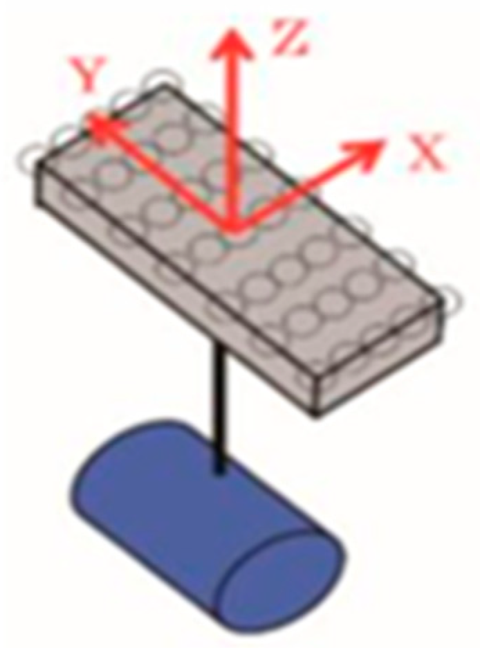
A 6-DOF robot arm comes in various types, such as RPY and PUMA models. The RPY type has two bending joints. Compared to the PUMA type, its mechanism is relatively larger. However, its wrist mechanism resembles that of a human wrist, making its movements easier to predict. Furthermore, when the wrist is straightened, it is less prone to singularities, resulting in easier task execution. On the other hand, the PUMA-type robot arm uses an Eulerian wrist mechanism, resulting in a compact wrist structure. However, its low wrist-axis stiffness makes it prone to vibration. Therefore, this study targets the control of RPY-type robot arms, aiming for high-axis stiffness and replicating the motion of the human wrist. The 6-axis force sensor is incorporated into the end-effector and is indicated by the rectangular prism at the tip, shown in Figure 1 and Figure 2.

2.2. Inverse Kinematics Using the Iterative Search Method

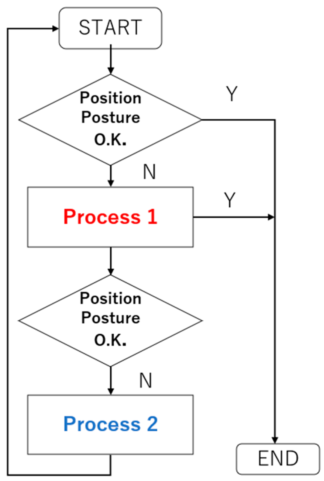
To apply hybrid control of position, orientation, force, and moment to a manipulator, solving the inverse kinematics is necessary. Therefore, we first consider solving the inverse kinematics problem for an RPY manipulator. The Newton–Raphson method is a well-known approach for solving such problems. However, this section proposes an alternative efficient solution: the sequential search method. This method converges ${\theta }_0$ = ${\theta }_1$[0] ⋯ ${\theta }_6$[0] to match the target position and orientation by repeatedly performing the following two processes, given the initial values ${\theta }_0$, ${\theta }_1$[0] ⋯ ${\theta }_6$[0] for each joint.

Process 1 focuses solely on modifying the position, completely ignoring the orientation. Process 2 focuses solely on modifying the orientation, completely ignoring the position. This processing flow is represented in a flowchart in Figure 3.

2.2.1. Process 1

In Process 1, ${\theta }_4$, ${\theta }_5$, and ${\theta }_6$ are fixed, and only ${\theta }_1$, ${\theta }_2$, and ${\theta }_3$ are modified. Specifically, ${\theta }_{\mathrm{k}+1}$ is calculated from ${\theta }_{\mathrm{k}}$ using the following equation.

$$p_k=\Lambda \left({\theta }_k\right)$$

(1)

$$\Delta p=p_{ref}-dt+p_k$$

(2)

$$p_{k+1}=p_k+w_p\Delta p$$

(3)

$${\theta }_{k+1}={{\Lambda }_{3p}}^{-1}(p_{k+1},{\theta }_4,{\theta }_5,{\theta }_6)$$

(4)

Equation (1) calculates $p_{\mathrm{k}}$ from ${\theta }_{\mathrm{k}}$ using forward kinematics. The following Equation (3) calculates the difference $\Delta p_{\mathrm{k}}$ from the target position, multiplies it by the weight $W_p$, and adds it to $p_{\mathrm{k}}$ to obtain the intermediate target position $p_{\mathrm{k}+1}$ via Equation (4). Finally, ${\theta }_{\mathrm{k}+1}$ is calculated using Equation (4) to align the end-effector position with $p_{\mathrm{k}+1}$. The ${{\Lambda }_{3p}}^{-1}$ in Equation (4) represents the inverse kinematics of the position when joints ${\theta }_4$, ${\theta }_5$, and ${\theta }_6$, and can be expressed as the function shown below.

$$\left[\begin{array}{c}{\theta }_1\\ {\theta }_2\\ {\theta }_3\end{array}\right]={{\Lambda }_{3p}}^{-1}(\left[\begin{array}{c}{x}_r\\ y_r\\ z_r\end{array}\right],\left[\begin{array}{c}{x}_a\\ y_a\\ z_a\end{array}\right],L_1,L_2)$$

(5)

$$\left[\begin{array}{c}{x}_r\\ y_r\\ z_r\end{array}\right]=p_{k+1}$$

(6)

$$\left[\begin{array}{c}{x}_a\\ y_a\\ z_a\end{array}\right]={\left(R_Z\left({\theta }_1\right),R_X\left({\theta }_2\right),R_X\left({\theta }_3\right)\right) }^T(p_k-{\left(p_3\right)}_k)$$

(7)

$$L_{\alpha }=\sqrt{{x_r}^2+{y_r}^2}$$

(8)

$${\theta }_{\alpha }=atan2(y_r,x_r)$$

(9)

$$\alpha ={sin}^{-1}\left({\displaystyle \frac{x_a}{L_a}}\right)-{\displaystyle \frac{\pi }{2}}$$

(10)

$$L_{\beta }=\sqrt{{z_a}^2+{y_a}^2}$$

(11)

$${\theta }_{\beta }=atan2(y_a,z_a)$$

(12)

$$z_{r2}=z_r-L_1$$

(13)

$$y_{r2}=-x_{r}sin\left(\alpha +{\theta }_{\alpha }\right)+y_{r}cos(\alpha +{\theta }_{\alpha })$$

(14)

$$\beta ={sin}^{-1}\left({\displaystyle \frac{y_{r2}^2{+z}_{r2}^2-L_{\beta }^2-L_2^2}{2L_{\beta }{L}_2}}\right)-{\displaystyle \frac{\pi }{2}}$$

(15)

$$L_{\beta }=\sqrt{y_{r2}^2{+z}_{r2}^2}$$

(16)

$${\theta }_{\gamma }=atan2(-L_{\beta }sin\beta {,L}_{\beta }cos\beta +L_2)$$

(17)

$$\gamma ={sin}^{-1}\left({\displaystyle \frac{z_{r2} }{L_{\gamma }}} \right) -{\displaystyle \frac{\pi }{2}}$$

(18)

However, atan2 is a two-variable function with a domain of −π ≤ θ ≤ π, defined as follows:

$$atan2\left(a,b\right)=\left\{\begin{array}{cc}{\tan }^{-1}\left({\displaystyle \frac{a}{b}}\right)\hfill & if b>0\hfill \\ {\displaystyle \frac{\pi }{2}}sign\left(a\right)\hfill & if b=0\hfill \\ {\tan }^{-1}\left({\displaystyle \frac{a}{b}}\right)+\pi \hfill & if b<0 \bigwedge a>0 \hfill \\ {\tan }^{-1}\left({\displaystyle \frac{a}{b}}\right)-\pi \hfill & if b<0 \bigwedge a>0 \hfill \end{array}\right.$$

Ultimately,

Table 1. Four possible solutions.

No.	1	2	3	4
${\theta }_1$	$\alpha +{\theta }_{\alpha }$	$\alpha +{\theta }_{\alpha }$	$-\alpha +{\theta }_{\alpha }$	$-\alpha +{\theta }_{\alpha }$
${\theta }_2$	$\gamma +{\theta }_{\gamma }$	$\gamma -{\theta }_{\gamma }$	$-\gamma +{\theta }_{\gamma }$	$-\gamma -{\theta }_{\gamma }$
${\theta }_3$	$\beta +{\theta }_{\gamma }$	$-\beta +{\theta }_{\gamma }$	$\beta +{\theta }_{\gamma }$	$-\beta +{\theta }_{\gamma }$

provides four possible values for ${\theta }_{k+1}$.

2.2.2. Process 2

In Process 2, ${\theta }_4$, ${\theta }_5$ and ${\theta }_6$ are fixed, and only ${\theta }_1$, ${\theta }_2$, and ${\theta }_3$ are adjusted. Let $R_{\mathrm{r}\mathrm{e}\mathrm{f}}$ denote the matrix representation of the target posture.

Then, the transition from ${\theta }_{\mathrm{k}}$ to ${\theta }_{\mathrm{k}+1}$ can be calculated using the following equation.

$$R_k=\Lambda \left({\theta }_k\right)$$

(19)

$$R_{err}={R_k}^T{R}_{ref}$$

(20)

$$∆\omega ={{\Lambda }_{\omega }}^{-1}\left(R_{err}\right)$$

(21)

$${\overline{R}}_{err}={\Lambda }_{\omega }\left(W_p ∆\omega \right)$$

(22)

$$R_{k+1}=R_k{\overline{R}}_{err}$$

(23)

$${\theta }_{k+1}={{\Lambda }_{3o}}^{-1}\left(R_{k+1},{\theta }_1{\theta }_2{\theta }_3\right) -{\displaystyle \frac{\pi }{2}}$$

(24)

First, we explain ${\Lambda }_{\omega }$. In general, a rotation matrix is equivalent to a rotation about a single axis. If we denote the unit vector in the direction of the rotation axis as u and the rotation angle as ${\theta }_{\mathrm{u}}$, then the vector ω = ${\theta }_{\mathrm{u}}$u can be interconverted with the rotation matrix. Therefore, if we denote the transformation from ω to $R$ as ${\Lambda }_{\omega }$, then ${\Lambda }_{\omega }$ and its inverse transformation ${{\Lambda }_{\omega }}^{-1}$ are given by the following equations:

$${\theta }_u=\left|\omega \right| u=\left[\begin{array}{c}{u}_x\\ u_y\\ u_z\end{array}\right]={\displaystyle \frac{\omega }{{\theta }_u}}$$

$${\Lambda }_{\omega }\left(\omega \right)=\left(1-cos{\theta }_u\right)u{u}^T+cos{\theta }_{u}I+sin{\theta }_u\left[\begin{array}{ccc}0& {-u}_z& u_y\\ u_z& 0& {-u}_x\\ {-u}_y& u_x& 0\end{array}\right]$$

(25)

$$R=\left[\begin{array}{ccc}r11& r12& r13\\ r21& r22& r23\\ r31& r32& r33\end{array}\right] d=\left[\begin{array}{c}r32-r23\\ r13-r31\\ r21-r12\end{array}\right]$$

$${{\Lambda }_{\omega }}^{-1}(R)={sin}^{-1}\left({\displaystyle \frac{\left|d\right|}{2}}\right){\displaystyle \frac{d}{\left|d\right|}}$$

(26)

Using this ${\Lambda }_{\omega }$ and weight $W_{\mathrm{p}}$, the intermediate target posture is determined, and ${\theta }_{\mathrm{k}+1}$ is calculated using the inverse kinematics ${{\Lambda }_{3\mathrm{o}}}^{-1}$ of the posture when joints ${\theta }_1$, ${\theta }_2$, and ${\theta }_3$ are fixed. The specific calculation procedure for ${{\Lambda }_{3\mathrm{o}}}^{-1}$ is shown below.

$$e_{4z}=R_Z\left({\theta }_1\right),R_X\left({\theta }_2\right),R_X\left({\theta }_3\right) \left[\begin{array}{c}0\\ 0\\ 1\end{array}\right]$$

(27)

$$e_{6z}=e_{7z}=R_{ref}\left[\begin{array}{c}0\\ 0\\ 1\end{array}\right]$$

(28)

$$\left[\begin{array}{c}{d}_{1x}\\ d_{1y}\\ d_{1z}\end{array}\right]={\left(R_Z\left({\theta }_1\right),R_X\left({\theta }_2\right),R_X\left({\theta }_3\right)\right) }^T{\displaystyle \frac{e_{4z}\times e_{6z}}{\left|e_{4z}\times e_{6z}\right|}}$$

(29)

$$\alpha =atan2(d_{1y},d_{1x})$$

(30)

$$\left[\begin{array}{c}{d}_{2x}\\ d_{2y}\\ d_{2z}\end{array}\right]={\left(R_Z\left({\theta }_1\right),R_X\left({\theta }_2\right),R_X\left({\theta }_3\right)\right) }^T{e}_{6z}$$

(31)

$$\beta =atan2(d_{2y},d_{2x})$$

(32)

$$\left[\begin{array}{c}{d}_{3x}\\ d_{3y}\\ d_{3z}\end{array}\right]={\left(R_Z\left({\theta }_1\right),R_X\left({\theta }_2\right),R_X\left({\theta }_3\right)\right) }^T{e}_{7z}$$

(33)

$$\gamma =atan2(d_{3y},d_{3x})$$

(34)

As a result of the above calculations, we obtain two solutions from

Table 2. Two possible solutions.

No.	1	2
${\theta }_4$	$\alpha$	$\alpha +\pi$
${\theta }_5$	$\beta$	$\pi -\beta$
${\theta }_6$	$\gamma$	$\gamma +\pi$

.

3. Hybrid Control in Previous Study

3.1. Avoiding Inverse Jacobian Matrix Calculation Using Differential Inverse Kinematics [26]

Before discussing hybrid control, we first describe the underlying position and posture control method. This study achieves position and posture control by solving inverse kinematics from target positions and postures to calculate the joint angle reference value ${\Theta }_{ref}$ and then by implementing PID control for each joint based on a differential inverse kinematics method. While methods using the inverse Jacobian matrix are known for position and posture control, they require handling singularities, which introduces new problems. Therefore, this study adopts a method that calculates the target angle values from the inverse kinematics. Specifically, the input torque ${\tau }_{po}$ is given by the following equation.

$${\Theta }_{ref}={\Lambda }^{-1}\left( {0p}_{7ref},{0R}_{7ref}\right)$$

(35)

$${\Theta }_{err}=K_p{\Theta }_{ref}-\Theta$$

(36)

$${\tau }_{po}=K_p{\Theta }_{err} +K_i\int {\Theta }_{err}dt+K_d{\dot{\Theta }}_{err}$$

(37)

The conventional position force hybrid control cannot be directly applied to the position and posture control discussed in the previous section. This is because the conventional method is not based on inverse kinematics control techniques, but rather on position and posture control using the inverse Jacobian matrix, as shown in the following equation.

$${\Theta }_{err}={ J}^{-1}[{0p}_{7err} { \phi }_{err}]$$

(38)

Therefore, to incorporate the position force hybrid control scheme into the equations, we adopt a method where the virtual target position, obtained by subtracting the force control direction error from the target position, becomes the new target position. That is,

$$0{\widehat{p}}_{7err}=Sp\left({0p}_{7ref}-{0p}_7\right)$$

(39)

$${0\widehat{p}}_{7ref}={ 0p}_7+{0\widehat{p}}_{7err}$$

(40)

$${\widehat{\Theta }}_{err}={\Lambda }^{-1}\left( {0\widehat{p}}_{7ref},{0R}_{7ref}\right)-\Theta$$

(41)

$${\tau }_{po}={ K}_p{\Theta }_{err}+K_i \int {\Theta }_{err}dt+K_d {\dot{\Theta }}_{err}$$

(42)

For force control, as in the conventional method

$$0{\widehat{f}}_{ err}=S_f\left( {0f}_{ref }-0f\right)$$

(43)

$${\tau }_f={{ J}_f}^{ T}(K_{fp} 0{\widehat{f}}_{ err}+K_{fi} \int 0{\widehat{f}}_{ err} dt+K_{fd }0{\dot{\widehat{f}}}_{ err})$$

(44)

Here, $S_f$ is the switch matrix for the force control direction, and $S_p=I-S_f$ is the switch matrix for the position control direction. ${ J}_{f }$ is the upper half of the Jacobian matrix and is a 3 × 6 matrix. The hybrid position force control is defined by adding the position and posture control torque ${\tau }_{po}$ and the force control torque ${\tau }_f$ to form the control input τ.

$$\tau ={\tau }_{po}+{\tau }_f$$

(45)

3.2. Freeing Posture Through Postural Component Decomposition [24]

In hybrid position force control, disabling position and posture control within the constrained space is termed freeing a certain direction. Position references are expressed using the switching matrices ${\mathrm{S}}_{\mathrm{p}}$ and ${\mathrm{S}}_{\mathrm{f}}$ as

$${\widehat{P}}_{ref}=S_p{p}_{ref}+S_{f}p$$

(46)

Here, $S_p$ and $S_f$ are 3 × 3 diagonal matrices where the components corresponding to the free space and the constrained space of the position are 1, respectively, and the rest are 0. However, for posture, the components cannot be calculated independently. The RPY representation of posture is nonlinear, and the calculation of the posture matrix changes depending on the order of operations. Therefore, simply defining

$${\widehat{\phi }}_{ref}=S_o{\phi }_{ref}+S_m\phi$$

(47)

is problematic.

To control the moment about a given u-axis and keep the posture about that axis free, the condition is

$${\widehat{R}}_{ref}=R(u,{\theta }_u)R_{ref}$$

(48)

Here, ${\widehat{R}}_{ref}$ is the virtual target posture, and $R(u,{\theta }_u)$ is the rotation matrix rotating by ${\theta }_u$ about the u-axis. To satisfy this condition, the decomposition order of the RPY must be chosen such that the rotation matrix for the axis to be kept free is applied last. Therefore, a switching matrix

$$S_m=diag(s_x,s_y,s_z)$$

(49)

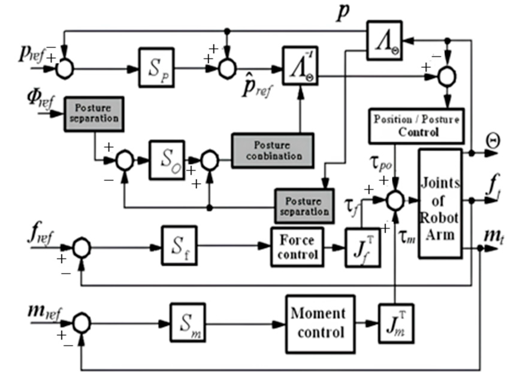
is used to dynamically change the decomposition order. Thus, an appropriate decomposition method and virtual target posture ${\widehat{R}}_{ref}$ are defined for each combination of switching matrices. This approach enables posture freedom in any direction, even within a control system based on differential inverse kinematics. Figure 3 shows a block diagram of the hybrid position and posture force control based on the differential inverse kinematics method and the posture component decomposition method.

3.3. Hybrid Control of Position, Posture, Force, and Moment [25]

From the virtual target position and posture obtained by the posture component separation method, the position control torque with position control to the constrained space disabled can be calculated using the following equation.

$${\widehat{\Theta }}_{ref}={{\Lambda }_{\Theta }}^{-1}({\widehat{p}}_{ref},{\widehat{R}}_{ref})$$

(50)

$${\widehat{\Theta }}_{ref}={\widehat{\Theta }}_{ref}-\Theta$$

(51)

$${\tau }_{po}=K_p{\widehat{\Theta }}_{ref}+K_i\int {\widehat{\Theta }}_{err}dt+K_d{\dot{\widehat{\Theta }}}_{err}$$

(52)

Furthermore, the force and moment control torques are calculated using the following equations, similar to the conventional method.

$$f_{err}=S_f(f_{ref}-f)$$

(53)

$$m_{err}=S_m(m_{ref}-m)$$

(54)

$${\tau }_f={J_f}^T(K_{fp}{f}_{err}+K_{fi}\int f_{err}dt)$$

(55)

$${\tau }_m={J_m}^T(K_{mp}{m}_{err}+K_{mi}\int m_{err}dt)$$

(56)

Here, $J_f$ and $J_m$ represent the upper and lower halves of the Jacobian matrix, respectively, and K is a diagonal matrix representing the PI gains for force and moment, respectively. The sum of these three torques is used as the control input. Then,

$$\tau ={\tau }_{po}{+\tau }_f{+\tau }_m$$

(57)

is obtained. The block diagram of this control system is shown in Figure 4.

4. Hybrid Control Using Dynamic Impedance

4.1. Introduction to Impedance Characteristics

When performing position and posture control, sliding friction exists as a disturbance. While this is not the primary cause of unstable vibrations in the robot arm’s end-effector, it does have a detrimental effect. Therefore, impedance characteristics accounting for this disturbance are introduced into the position and posture control to achieve stabilization. The position and posture acceleration targets are set as follows:

$${\ddot{X}}_{po}={\ddot{X}}_{ref} +{M_{i }}^{-1}\left(C_i\left({\dot{X}}_{ref} -{\dot{X}}_{po}\right)+K_i\left(X_{ref}-X_{po}\right)+F_d\right)$$

(58)

${K_i, C}_i, \mathrm{a}\mathrm{n}\mathrm{d}{ M}_{i }$ represent the stiffness, viscous damping, and inertia of the designed impedance, while $F_d$ is the contact force obtained from the force sensor. If the acceleration calculated by this equation can be achieved in free space, it is considered that the end-effector of the robot arm will possess impedance characteristics against disturbances, mitigating the effects of friction. Therefore,

$${ F}_i=\Lambda {\ddot{X} }_{po}$$

(59)

This input does not generate acceleration in the constrained

$$F=(I-S)F_i$$

(60)

In this case,

$$\begin{array}{c}SF=S\left(I-S\right)\Lambda {\ddot{X}}_{po}\\ =\left(S-SS\right)\Lambda {\ddot{X}}_{po}\\ =\left(S-S\right)\Lambda \ddot{X_{po}}\\ =0 \end{array}$$

(61)

$$\begin{array}{c}\left(I-S\right){\Lambda }^{-1}F=\left(I-S\right){\Lambda }^{-1}\left(I-S\right)\Lambda {\ddot{X} }_{po}\\ =\left(I-S\right)\left({\Lambda }^{-1}-{\Lambda }^{-1}S\right)\Lambda {\ddot{X}}_{po }\\ =\left(I-S\right)\left({\Lambda }^{-1}-{\Lambda }^{-1}S\right)\Lambda {\ddot{X}}_{po }\\ =\left(I-S\right){\ddot{X}}_{po }-\left(1-S\right){T_s}^T{\left(T_s\Lambda {T_s}^T\right)}^{-1}\Lambda {\ddot{X}}_{po }\\ =\left(I-S\right){\ddot{X}}_{po }-\left({T_s}^T-{T_s}^T\right){\left(T_s\Lambda {T_s}^T\right)}^{-1}{T}_s\Lambda {\ddot{X}}_{po }\\ =(I-S){\ddot{X}}_{po }\end{array}$$

(62)

Therefore, switching S allows eliminating force and moment interference inputs to the constrained space without altering the input acceleration for position and posture control.

4.2. Dynamization of Design Impedance Stiffness Based on the Final Value Theorem for Steady-State Deviation

When the equation of motion in joint coordinate space

$$M\left(\theta \right)\ddot{\theta }+C\left(\theta ,\dot{\theta }\right)+U\left(\theta \right)+D\left(\dot{\theta }\right)+N\left(\dot{\theta }\right)=\tau$$

(63)

is transformed into the equation of motion in Cartesian coordinate space using the Jacobian matrix, we obtain

$$J^{-T}M\left(\theta \right)J^{-1}\ddot{X}-J^{-T}+J^{-T}M\left(\theta \right)J^{-1}J{J}^{-1}\dot{X}(C\left(\theta ,\dot{\theta }\right)+U\left(\theta \right)+D\left(\dot{\theta }\right)+N\left(\dot{\theta }\right))=F$$

(64)

$$\Lambda \ddot{X}+H=F$$

(65)

Further transforming this yields

$$\ddot{X}={\Lambda }^{-1}(F-H)$$

(66)

The ${\Lambda }^{-1}$ in Equation (66) is generally not a diagonal matrix.

Defining $X_e=X_{ref}-X_{po}$ and applying the Laplace transform yields

$$\left(M_i{s}^2+C_{i}s+K_i\right)=X_e\left(s\right)=F_d\left(s\right)$$

(67)

In Equation (58), the disturbance force $F_d$ acting on the end-effector $F_d$ is the projection of the inertial and viscous terms in joint space onto the workspace via $J^T$

$$F_d\left(s\right)={\displaystyle \frac{M}{J^T}}{s}^2\theta \left(s\right)+{\displaystyle \frac{D}{J^T}}s\theta (s)$$

(68)

This yields Equation (21) below

$$X_e(s)={\displaystyle \frac{\frac{M }{J^T}{s}^2\theta (s)+\frac{D }{J^T}s\theta (s) }{M_i{s}^2+C_{i}s+K_i}}$$

(69)

where K is the design parameters, D is the dynamic friction coefficient, ${\mathit{J}}^{\mathit{T}}$ is the Jacobian matrix, $\mathsf{\zeta }$ is the damping coefficient, and ${\mathit{\omega }}_{\mathit{n}}$ represents the natural frequency.

Furthermore, determine the value of $K_i$ that enhances stability using the final value theorem for steady-state error.

$$s{X}_e\left(s\right)=\underset{s\to 0}{\mathit{lim}}{\displaystyle \frac{\frac{M}{J^T}{s}^3\theta \left(s\right)+\frac{D }{J^T}{s}^2\theta \left(s\right)}{M_i{s}^2+C_{i}s+K_i}}$$

(70)

In the wall-wiping task, the joints move at an approximately constant angular velocity, which corresponds to a ramp input $\theta (s)={\displaystyle \frac{a}{s^{ 2}}}$ where a is the angular acceleration. Substituting this into Equation (71):

$$x_e(t) = {\displaystyle \frac{\frac{D}{J^T} a}{K_i}}$$

(71)

Since stability increases as $x_e\left(t\right)$ approaches 0,

$$K_i \gg {\displaystyle \frac{D}{J^T}}a$$

(72)

is desirable.

In this study,

$$K_i=K{\displaystyle \frac{D}{J^T}}$$

(73)

is adopted.

4.3. Dynamization of Design Impedance Viscosity, and Inertia Based on Second-Order-Form Transient Response

The values of ${\mathbf{M}}_{\mathbf{i}}$ and ${\mathbf{C}}_{\mathbf{i}}$ for stability improvement are determined using the transient response of the quadratic form. The transfer function of a stable quadratic form is

$$\mathit{G}(\mathit{s})={\displaystyle \frac{\mathit{K}{{\mathit{\omega }}_{\mathit{n}}}^2}{{\mathit{s}}^2+2\mathit{\zeta }{\mathit{\omega }}_{\mathit{n}}\mathit{s}+{{\mathit{\omega }}_{\mathit{n}}}^2}}$$

(74)

The transfer function of the robotic arm is

$$X_e(s)={\displaystyle \frac{\frac{M }{J^T}{s}^2\theta (s)+\frac{D }{J^T}s\theta (s)}{s^2+\frac{C_i}{M_i} s+\frac{K_i}{M_i} }}$$

(75)

Since the robot arm transfer function should be in the same form as a stable quadratic transfer function, the following two equations are obtained and are shown as the following equations.

$${{\omega }_n}^2={\displaystyle \frac{K_i}{M_i}}$$

(76)

$$2\zeta {\omega }_n=C_i M_i$$

(77)

Therefore,

$$M_i={\displaystyle \frac{ KD}{{{J^T\omega }_n}^2}}$$

(78)

$$C_i={\displaystyle \frac{2\zeta KD}{{J^T\omega }_n}}$$

(79)

5. Simulation Environment

5.1. 6-DOF 3D Dynamic Model

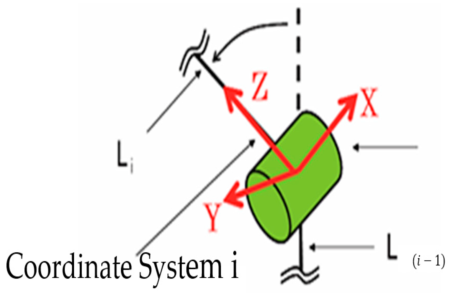
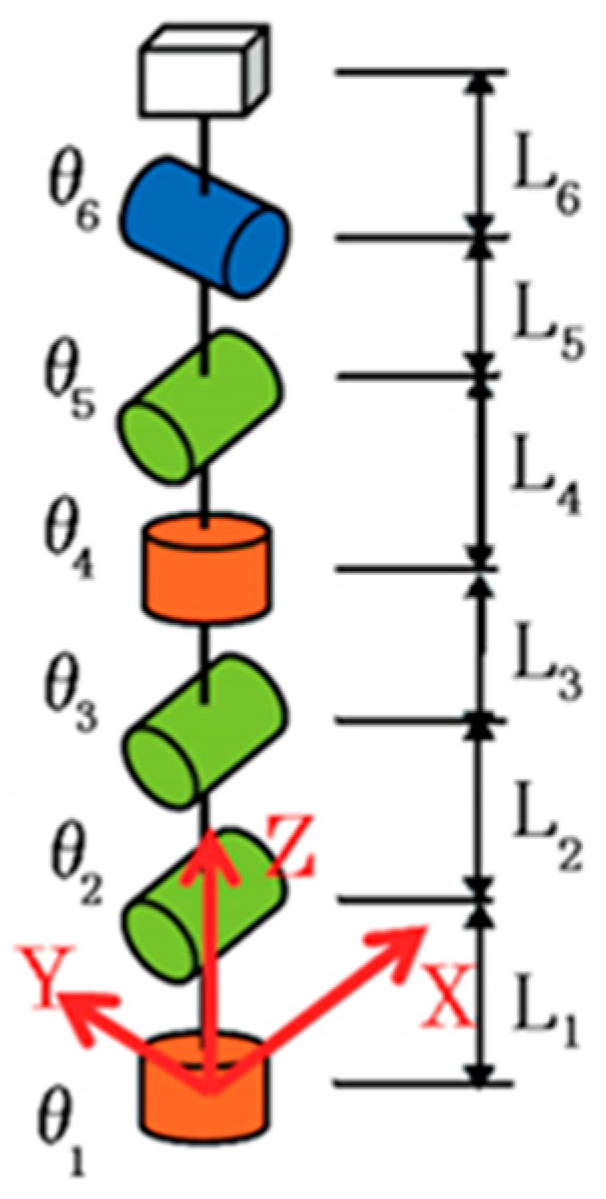
To create a dynamic model of the manipulator, we first derive the equations of motion using the Lagrange multiplier method. To do this, we first define the joint coordinate system as shown in Figure 5.

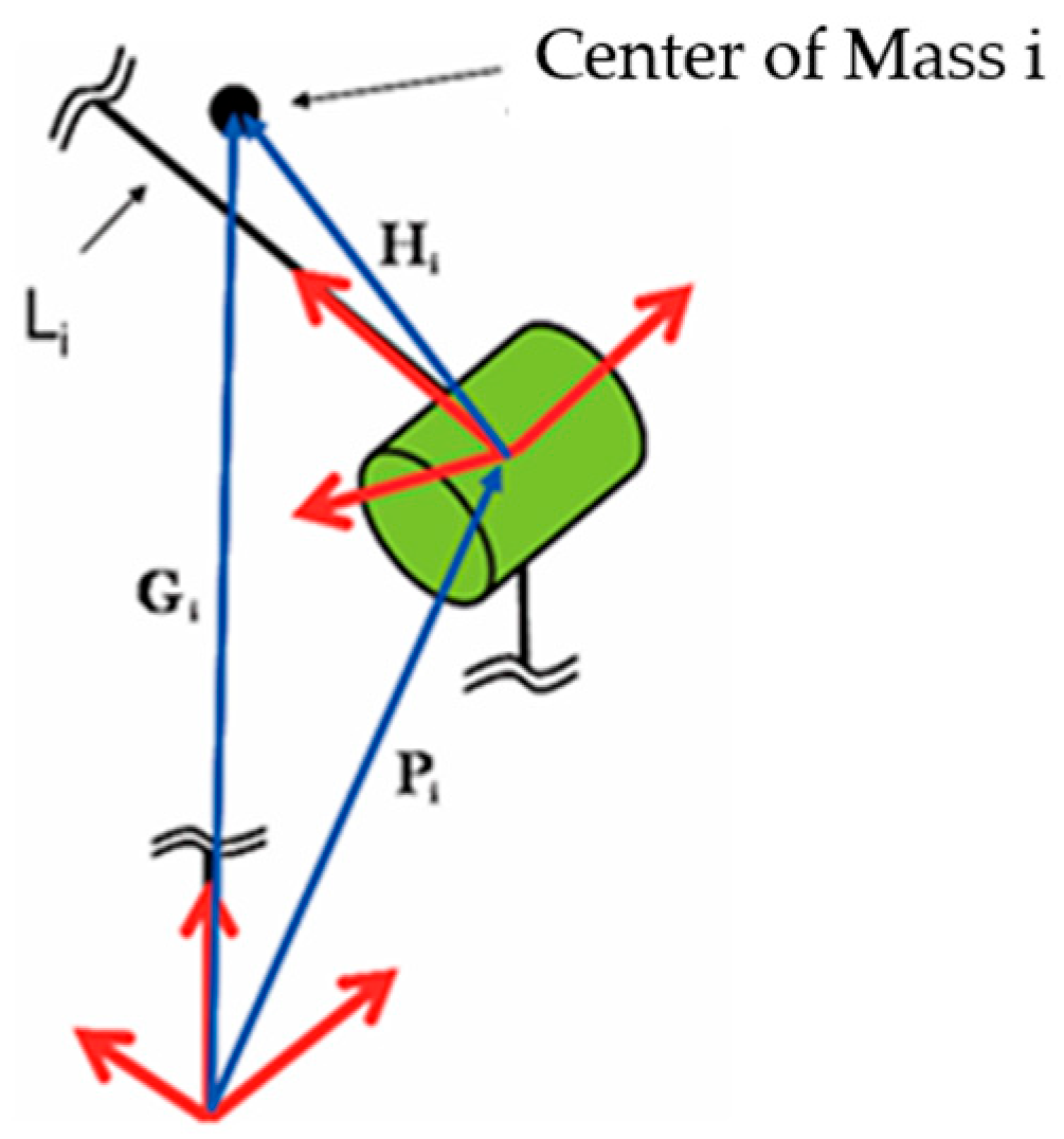
As shown in Figure 5, coordinate system i is fixed to link i, and the direction of the link’s length aligns with the z-axis. Furthermore, in Figure 6, Gi and Hi represent the position of the center of mass i in the absolute coordinate system and the joint coordinate system i, respectively. Additionally, pi represents the position of joint i; more precisely, it represents the position of the origin of coordinate system i. Furthermore, the intrinsic angular velocity vectors and rotation matrices generated by each joint are defined as follows.

$${\omega }_1=\left[\begin{array}{c}0\\ 0\\ {\dot{\theta }}_1\end{array} \right] {\omega }_2=\left[\begin{array}{c}{\dot{\theta }}_1\\ 0\\ 0\end{array} \right] {\omega }_3=\left[\begin{array}{c}{\dot{\theta }}_1\\ 0\\ 0\end{array} \right]$$

(80)

$${\omega }_1=\left[\begin{array}{c}0\\ 0\\ {\dot{\theta }}_4\end{array} \right] {\omega }_2=\left[\begin{array}{c}{\dot{\theta }}_5\\ 0\\ 0\end{array} \right] {\omega }_3=\left[\begin{array}{c}0\\ {\dot{\theta }}_6\\ 0\end{array} \right]$$

(81)

$$R_1=\left[\begin{array}{ccc}cos{\theta }_1& -sin{\theta }_1& 0\\ sin{\theta }_1& cos{\theta }_1& 0\\ 0& 0& 1\end{array} \right] R_2=\left[\begin{array}{ccc}1& 0& 0\\ 0& cos{\theta }_2& -sin{\theta }_2\\ 0& sin{\theta }_2& cos{\theta }_2\end{array}\right]$$

(82)

$$R_3=\left[\begin{array}{ccc}1& 0& 0\\ 0& cos{\theta }_3& -sin{\theta }_3\\ 0& sin{\theta }_3& cos{\theta }_3\end{array} \right] R_4=\left[\begin{array}{ccc}cos{\theta }_4& -sin{\theta }_4& 0\\ sin{\theta }_4& cos{\theta }_4& 0\\ 0& 0& 1\end{array} \right]$$

(83)

$$R_5=\left[\begin{array}{ccc}1& 0& 0\\ 0& cos{\theta }_5& -sin{\theta }_5\\ 0& sin{\theta }_5& cos{\theta }_5\end{array} \right] R_6=\left[\begin{array}{ccc}cos{\theta }_6& 0& sin{\theta }_6\\ 0& 1& 0\\ -sin{\theta }_6& 0& cos{\theta }_6\end{array}\right]$$

(84)

Furthermore, let the mass and inertia tensor of each joint be denoted by mi and Ii, respectively. Based on these definitions, the translational kinetic energy Tt and rotational kinetic energy Tr of each link shown in Figure 6 can be calculated as follows:

$$p_1 =0$$

(85)

$$p_{i+1}=p_1+R_1\dots R_i{H}_i$$

(86)

$$T_t=\sum _{i=1}^6({\displaystyle \frac{1}{2}}{m}_i{G_i}^T{G_i}^T)$$

(87)

$${\mathit{\Omega }}_1={\omega }_1$$

(88)

$${\mathit{\Omega }}_1={\mathit{\Omega }}_i+{R_i}^T{\mathit{\Omega }}_{i-1}$$

(89)

$$T_r=\sum _{i=1}^6({\displaystyle \frac{1}{2}}{{\mathit{\Omega }}_i}^T{I}_i{\mathit{\Omega }}_i)$$

(90)

Ωi is the angular velocity vector of link I, as seen from joint coordinate system i. Furthermore, the gravitational potential energy U and the viscous loss energy D are given by the following equations.

$$U=\sum _{i=1}^6(m_i\left[\begin{array}{ccc}0& 0& g\end{array}\right]G_i)$$

(91)

$$D={\displaystyle \frac{1}{2}}{\dot{\theta }}^{T}Q\dot{\theta }$$

(92)

However, Q is a diagonal matrix consisting of the viscous friction coefficients at each joint, and g is the acceleration due to gravity. Substituting these energies into the Lagrangian equations yields the following equations of motion.

$${\displaystyle \frac{d}{dt}} \left({\displaystyle \frac{\mathsf{\partial }T}{\mathsf{\partial }\dot{\theta }}}\right)-{\displaystyle \frac{\mathsf{\partial }T}{\mathsf{\partial }\theta }}+{\displaystyle \frac{\mathsf{\partial }U}{\mathsf{\partial }\theta }}+{\displaystyle \frac{\mathsf{\partial }D}{\mathsf{\partial }\dot{\theta }}}=\tau$$

(93)

$$M\left(\theta \right)\ddot{\theta }=C\left(\theta ,\dot{\theta }\right)+U\left(\theta \right)+D\left(\dot{\theta }\right)=\tau$$

(94)

Furthermore, when dry friction is taken into account, the equation becomes

$$M\left(\theta \right)\ddot{\theta }=C\left(\theta ,\dot{\theta }\right)+U\left(\theta \right)+D\left(\dot{\theta }\right)+N\left(\dot{\theta }\right)=\tau$$

(95)

$$N\left(\dot{\theta }\right)=\left[\begin{array}{c}{N}_{1}sgn\left({\dot{\theta }}_1\right)\\ N_{2}sgn\left({\dot{\theta }}_2\right)\\ \begin{array}{c}{N}_{3}sgn\left({\dot{\theta }}_3\right)\\ N_{4}sgn\left({\dot{\theta }}_4\right)\\ \begin{array}{c}{N}_{5}sgn\left({\dot{\theta }}_5\right)\\ N_{6}sgn\left({\dot{\theta }}_6\right)\end{array}\end{array}\end{array}\right]$$

(96)

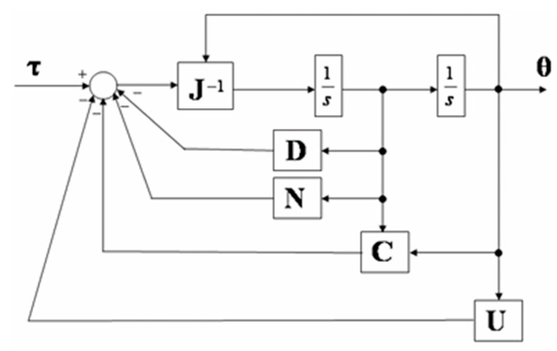
and Ni represents the kinetic friction coefficient at each joint. Using the equation of motion derived here, a dynamic analysis is performed on the system, shown in the block diagram in Figure 7.

5.2. RPY-Type 6-DOF Robot Arm Model

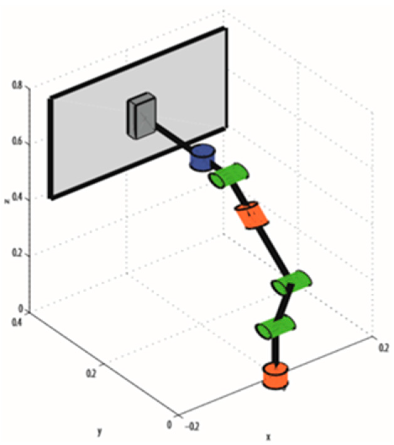
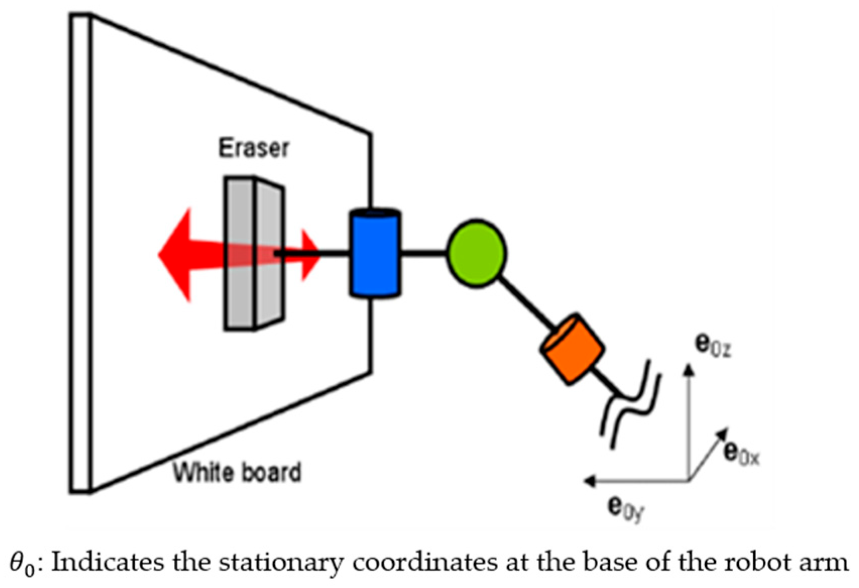
This section models the contact forces between the end-effector and the external environment during face-to-face contact. This study verifies the effectiveness of hybrid control of position, posture, force, and moment by performing whiteboard eraser motion with the end-effector in planar contact with a wall, as shown in Figure 8. The end-effector is rectangular, with lengths in the x- and y-directions of 4 cm and 12 cm, respectively, as shown in Figure 9. In this study, as shown in Figure 9, we employ a method for calculating surface contact forces by setting 35 grid points on the end-effector as contact points and synthesizing the forces received at each point. Figure 10 shows the angles and lengths of the robot used in this simulation. The specific values are shown in

Table 3. Length and weight of each link.

Link	Length [m]	Weight [kg]
${\mathit{L}}_{\mathbf{1}}$	0.175	2.717
${\mathit{L}}_{\mathbf{2}}$	0.2	1.231
${\mathit{L}}_{\mathbf{3}}$	0.18	1.498
${\mathit{L}}_{\mathbf{4}}$	0.105	0.821
${\mathit{L}}_{\mathbf{5}}$	0.07	0.807
${\mathit{L}}_{\mathbf{6}}$	0.174	0.900

. The force that each contact point receives from the wall is calculated using a damper model. The analytical model of the RPY-type robotic arm is created by using MATLAB/Simulink.

The method for calculating the force at the contact point is described below [12]. The position p_p of the contact point can be easily determined using kinematics, and the velocity v_p using the Jacobian matrix. Let p_wall denote the vector perpendicular to the wall. The amount δ by which the contact point penetrates the wall and its velocity $\dot{\mathit{\delta }}$ are given by:

$$\delta ={\displaystyle \frac{p_{wall}\cdot p_p}{|p_{wall}|}}-|p_{wall}|$$

(97)

$$\dot{\delta }={\displaystyle \frac{p_{wall}\cdot p_p}{\left|p_{wall}\right|}}$$

(98)

This leads to the spring and damper coefficients K_w and C_w between the wall and the contact point,

$$f_P=(K_w\delta +C_w\dot{\delta }){\displaystyle \frac{p_{wall}}{\left|p_{wall}\right|}}$$

(99)

Calculate the compression force acting toward the wall. Here, the condition for the compression force to act is

$$\delta >0 \wedge fp>0$$

This is expressed as f_p = 0 when the condition is not satisfied. The left equation represents the condition of contact with the wall, while the right equation indicates that the contact point is not being pulled toward the wall. Below, we derive the equation for the friction force parallel to the wall.

$$\sigma =v_p-{\displaystyle \frac{p_{wall}}{\left|p_{wall}\right|}}({\displaystyle \frac{p_{wall}}{\left|p_{wall}\right|}}{\dot{v}}_p)$$

(100)

$$f_f=|f_P|Fric(|\sigma |){\displaystyle \frac{\sigma }{|\sigma |}}$$

(101)

where σ represents the component of the contact point velocity parallel to the wall. Furthermore, shown as Equation (36), Fric(|σ|) is a function that relates sliding velocity to the coefficient of kinetic friction. We set the coefficient of static friction to µ1 = 0.4, the coefficient of kinetic friction independent of velocity to µ2 = 0.3, and the velocity-dependent coefficient of kinetic friction to µ3 = 0.2. From the above, the force acting from the contact point to the wall is obtained as

$${\mu }_{\left(v\right)}=\mathit{min}\left({\displaystyle \frac{{\mu }_1}{v_{dry}}},{\mu }_2\right)+({\mu }_1-{\mu }_2)e^{{-\left(v_{dry}-v\right)}^{40}})+{\mu }_{3}v$$

(102)

$$f_c=f_P+f_f$$

(103)

The moment is calculated using the following equation:

$$p_a=p_p-{\displaystyle \frac{p_{wall}}{\left|p_{wall}\right|}}\left({\displaystyle \frac{p_{wall}}{\left|p_{wall}\right|}}{\dot{v}}_p\right)+p_{wall}$$

(104)

$$m_c=(p_a-p)$$

(105)

Here, p_a represents the point of force application. Assuming the wall is sufficiently rigid compared to the end-effector, allowing deformation to be neglected, the point of force application is taken on the wall. This enables the verification of hybrid control of position, posture, force, and moment.

5.3. Analysis Method

The simulation uses a partial model that considers only the main shaft’s moment of inertia and gravity, simulate the end-effector’s surface on the wall using MATLAB/Simulink. Figure 11 show schematic of wall-wiping task and end-effector coordinate frame.

Table 4. Simulation conditions.

Simulation Time [s]	$\mathit{t}$: 0.8
Target position [m]	$x$: −0.14 $y$: 0.37 $z$: 0.6
Target posture [degree]	${\theta }_{Roll}$: 0 ${\theta }_{Pitch}$: 0 ${\theta }_{Yaw}$: 0
Force Target Value [N]	$F_y$: 10
Moment Target Value [Nm]	$M_x$: 0 $M_z$: 0

lists the simulation conditions.

${\theta }_0$: Indicates the stationary coordinates at the base of the robot arm

6. Simulation Results and Discussion

6.1. Comparison Before and After Applying Dynamic Impedance and Parameters

The analysis results for the position, posture, force, and moment of the robot arm before and after applying dynamic impedance are shown in Figure 12, Figure 13, Figure 14 and Figure 15, with ${\mathrm{K}}_{\mathrm{i}},{\mathrm{C}}_{\mathrm{i}}, \mathrm{a}\mathrm{n}\mathrm{d} {\mathrm{M}}_{\mathrm{i}}$ shown in Figure 16, Figure 17 and Figure 18. The parameters in conventional impedance control are indicated in

Table 5. Parameters in conventional impedance control.

	$\mathit{x}$	$\mathit{y}$	$\mathit{z}$	${\mathit{\theta }}_{\mathit{R}\mathit{o}\mathit{l}\mathit{l}}$	${\mathit{\theta }}_{\mathit{P}\mathit{i}\mathit{t}\mathit{c}\mathit{h}}$	${\mathit{\theta }}_{\mathit{Y}\mathit{a}\mathit{w}}$
$K_i$ [N/m]	0	10,000	0	10,000	0	10,000
$C_i$ [Ns/m]	0	1	0	1	0	1
$M_i$ [kg]	0	10	0	1	0	1

.

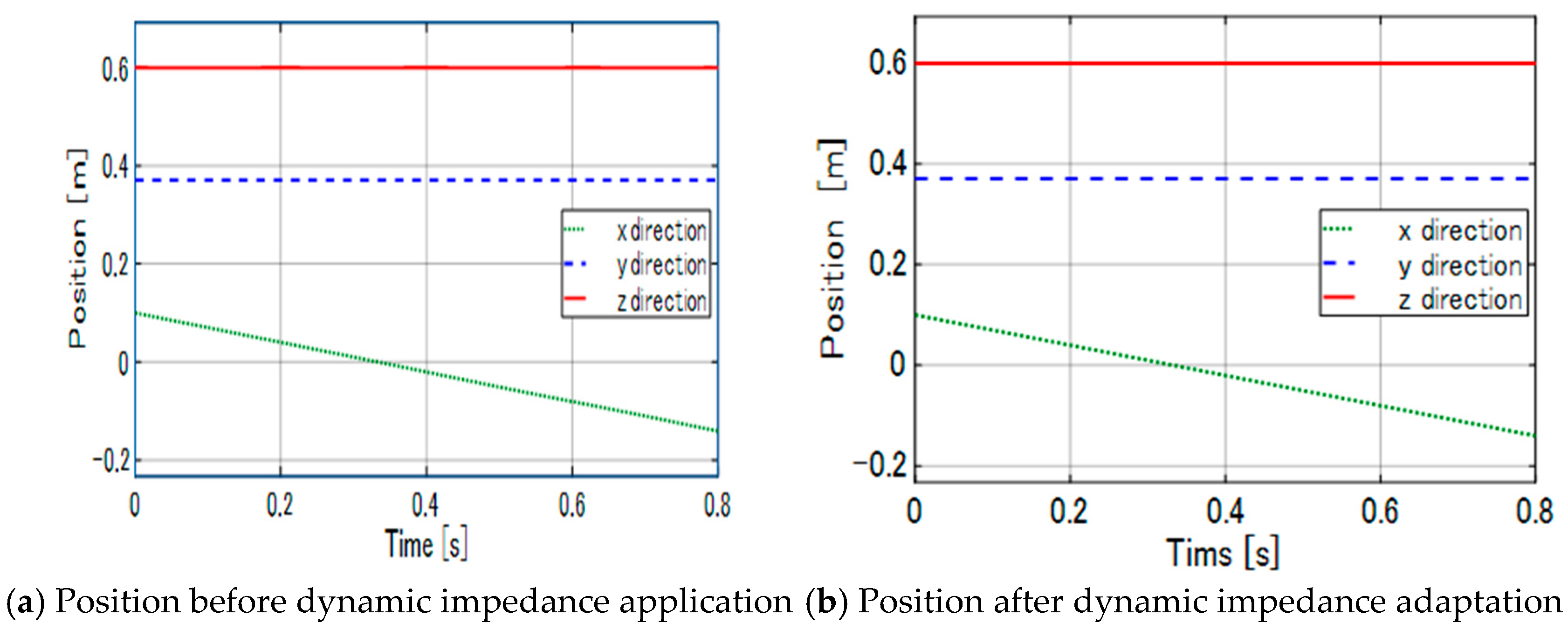
Figure 12 shows the positions in the x-, y-, and z-directions before and after applying dynamic impedance. No significant changes in position are observed before and after applying dynamic impedance. Regarding the position waveform in the x-direction, both start at approximately 0.1 m, decrease linearly with time, and reach a value of −0.14 m at 0.8 s. Regarding the position waveform in the y-direction, both maintain a constant value of 0.37 m over time. Regarding the position waveform in the z-direction, both before and after application, it shows a constant value of 0.6 m over time. The error relative to the target value at 0.8 s is $2.14\times {10}^{-3}\%$ for the x-direction, $5.35 \times { 10}^{-7}\%$ for the y-direction, and $3.07\times {10}^{-5}\%$ for the z-direction.

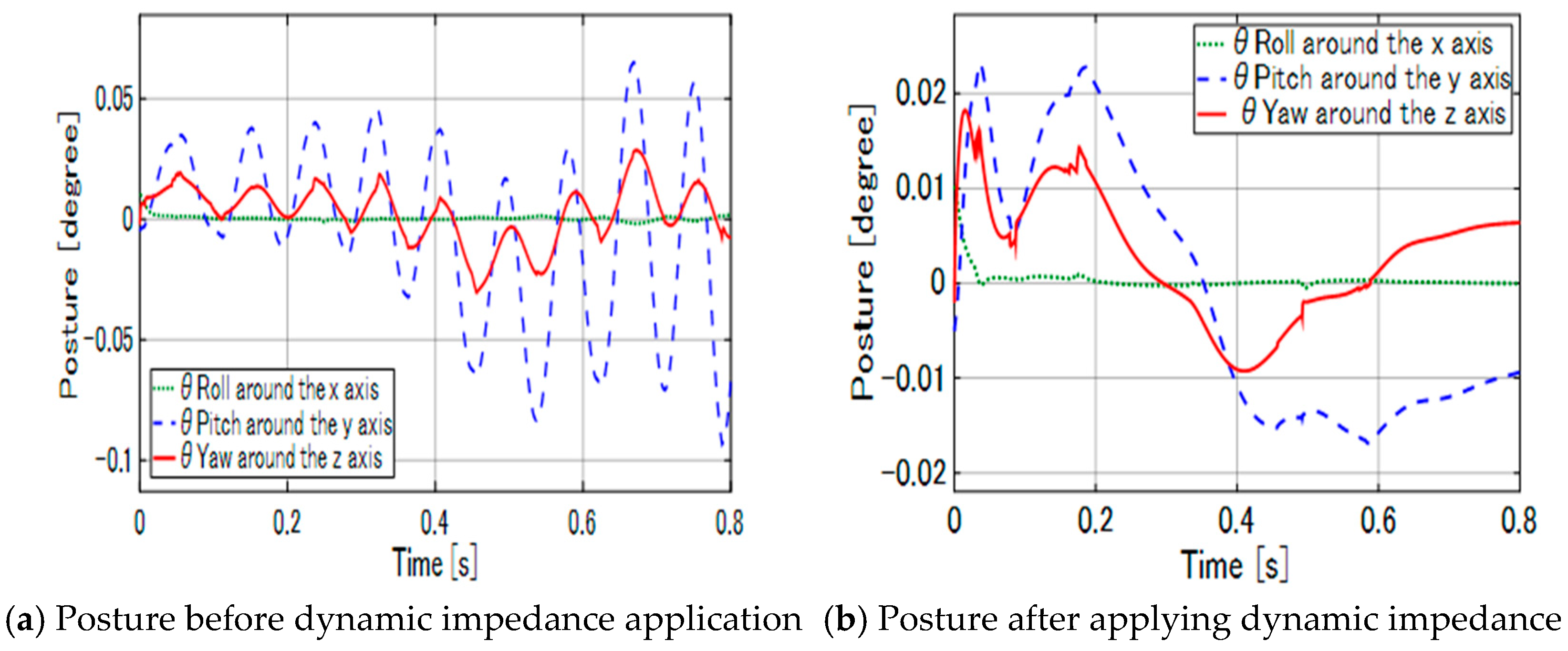
Figure 13 shows the waveforms of the roll angle ${\theta }_{Roll}$, pitch angle ${\theta }_{Pitch}$, and yaw angle ${\theta }_{Yaw}$ around the x-, y-, and z-axes, respectively, before and after applying dynamic impedance. The waveform of the roll posture angle ${\theta }_{Roll}$ around the x-axis before applying dynamic impedance shows a spike at the start of the simulation, but maintains a constant value of 0 degrees over time. In contrast, the waveform of ${\theta }_{Roll}$ around the x-axis after applying dynamic impedance exhibits a larger spike than before adaptation. While it maintains approximately 0 degrees over time, small spikes are visible. Regarding the pitch angle ${\theta }_{Pitch}$ waveform around the y-axis before dynamic impedance application, it oscillates over time. The amplitude increases as time progresses, reaching an amplitude of approximately −0.09 degrees from about 0.05 degrees at 0.7 s. In contrast, the waveform of the pitch posture angle ${\theta }_{Pitch}$ around the y-axis, after applying dynamic impedance adaptation, shows oscillation over time. However, it is significantly suppressed, with the maximum amplitude being approximately 0.02 degrees at 0.2 s. The waveform of the yaw posture angle ${\theta }_{Yaw}$ around the z-axis before applying dynamic impedance oscillates over time, reaching a maximum of approximately 0.025 degrees. In contrast, the waveform of the yaw posture angle ${\theta }_{Yaw}$ around the z-axis after applying dynamic impedance reaches around 0.02 degrees at the start of the simulation but shows reduced oscillation compared to before dynamic impedance application. When compared to the target values, the roll posture angle ${\theta }_{Roll}$ around the x-axis shows a large error at 0 s due to a spike, but the error stabilizes at around $1\times {10}^{-2} \left[\mathrm{d}\mathrm{e}\mathrm{g}\mathrm{r}\mathrm{e}\mathrm{e}\right]$ after 0 s. For the pitch posture angle ${\theta }_{Pitch}$ around the y-axis, the maximum error of $2.29\times {10}^{-2} \left[\mathrm{d}\mathrm{e}\mathrm{g}\mathrm{r}\mathrm{e}\mathrm{e}\right]$ occurs at 0.03 s, and for the yaw posture angle ${\theta }_{Yaw}$ around the z-axis, the maximum error of 1.81 $\times {10}^{-2} \left[\mathrm{d}\mathrm{e}\mathrm{g}\mathrm{r}\mathrm{e}\mathrm{e}\right]$ occurs at 0.18 s.

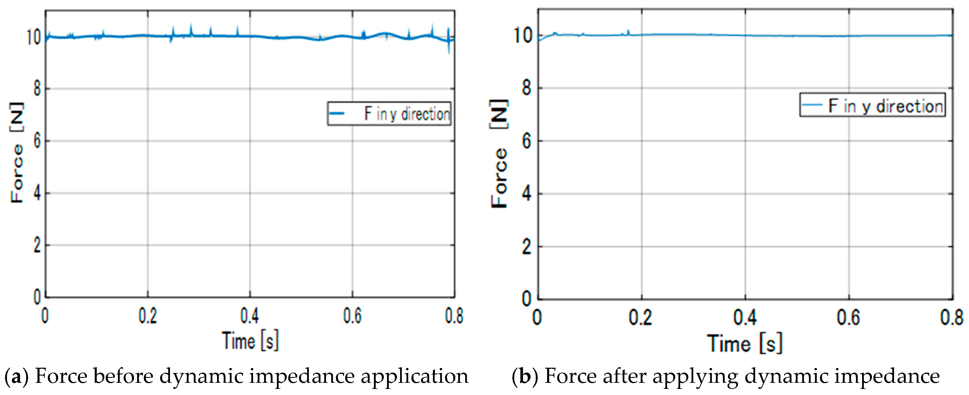
Figure 14 shows the force waveform in the y-direction after dynamic impedance adaptation. Examining the waveform before dynamic impedance adaptation reveals small spikes. Furthermore, between 0.5 s and 0.8 s, the waveform exhibits vibration, showing an error of approximately 1%. On the other hand, after dynamic impedance adaptation, it can be seen that the spikes occurring between 0.2 s and 0.4 s, which were present in the pre-adaptation waveform, have been improved. Additionally, improvement was observed in the waveform vibration seen between 0.5 s and 0.8 s. When compared to the target value, the maximum error is 2.05% at 0.17 s.

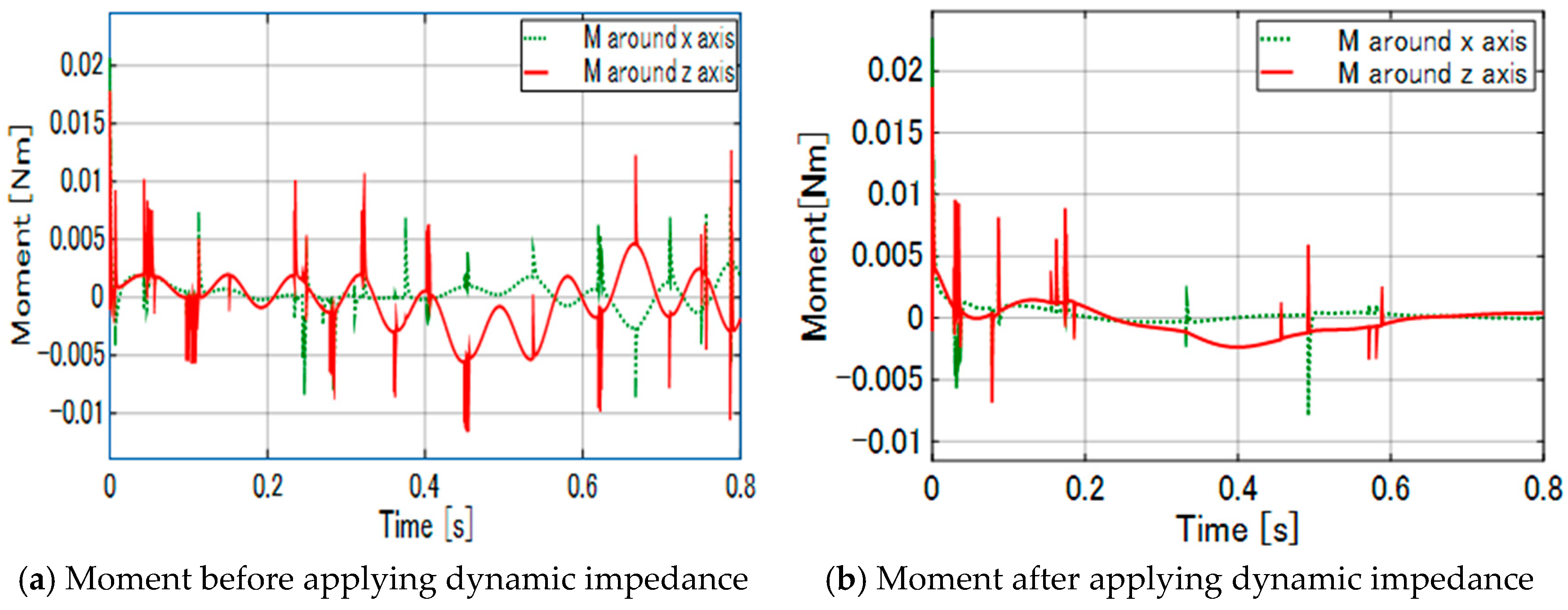
Figure 15 shows the moment waveforms in the $M_x around x axis$ and $M_z around z axis$ before and after applying dynamic impedance. The moment in the $M_x around x axis$ before applying dynamic impedance exhibits vibration over time, resulting in a waveform with prominent spikes. The largest spike rises to approximately 0.075 Nm around 0.75 s. In contrast, the moment waveform in the $M_x around x axis$ after applying dynamic impedance shows spikes at 0.05 s and 0.5 s, but this is stable at the target value of 0 Nm. The moment waveform in the $M_z around z axis$ before applying dynamic impedance exhibits significant oscillation over time. The simulation reveals numerous spikes, rising near 0.01 Nm or −0.075 Nm. In contrast, the moment waveform in the $M_z around z axis$ after applying dynamic impedance shows oscillations over time but converges to 0 Nm around 0.6 s. Although spikes still occur, they are significantly improved, with a substantial reduction in the number of spikes reaching values close to 0.01 Nm or −0.075 Nm. When compared to the target values, the maximum error for the moment in the $M_x around x axis$ is $1.0\times {10}^{-4} \left[\mathrm{N}\mathrm{m}\right]$ at 0.02 s, and for the $M_z around z axis$, it is 1.0 $\times {10}^{-2} \left[\mathrm{N}\mathrm{m}\right]$ at 0.017 s.

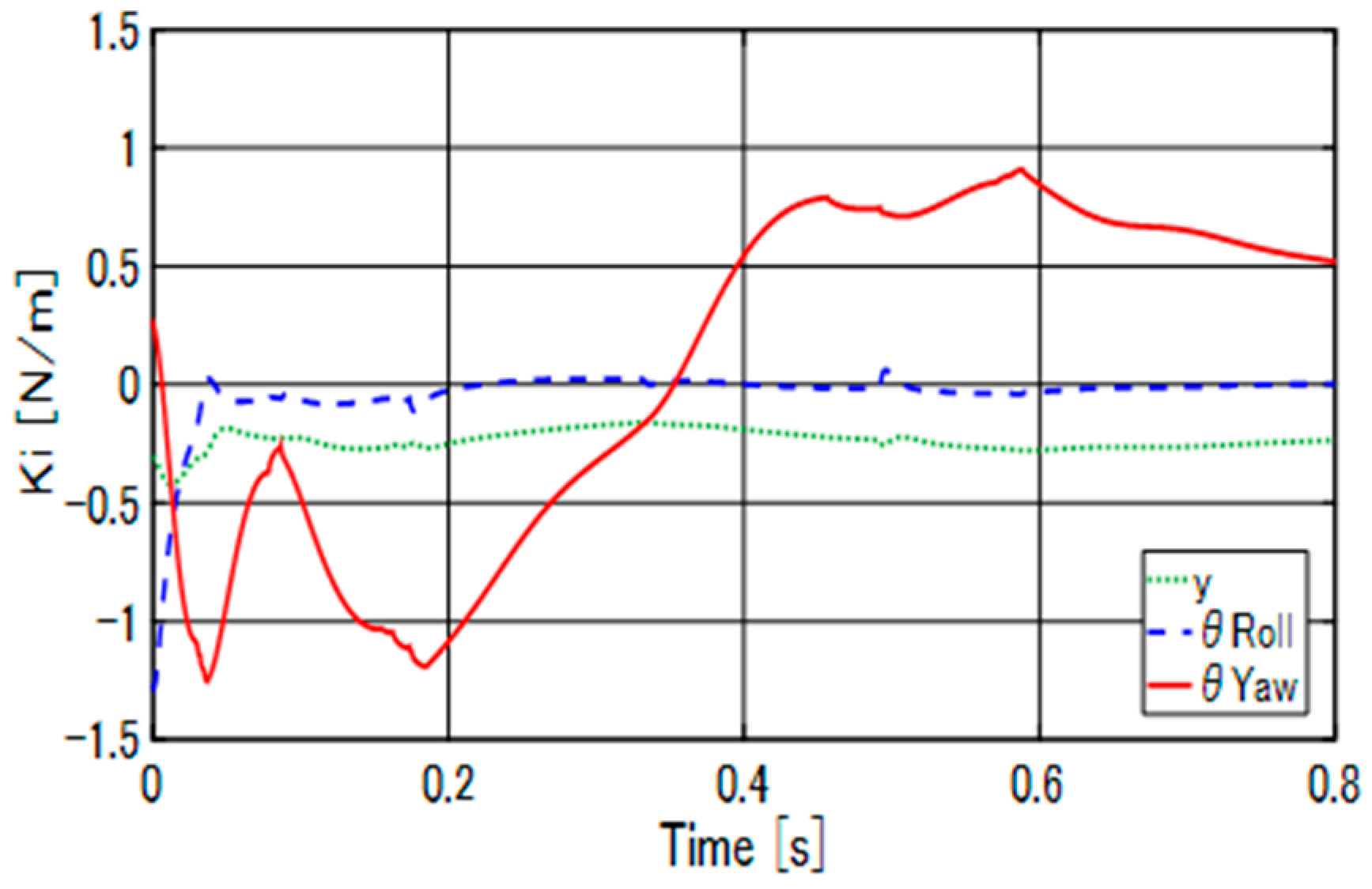
Figure 16 shows the dynamic $K_i$. For the y waveform, a slight oscillation is observed, but it maintains approximately −0.25 N/m throughout the simulation. For the ${\theta }_{Roll}$ waveform, it starts at approximately −1.25 N/m, reaches 0 N/m at about 0.05 s, and remains constant at 0 N/m with minor errors. The ${\theta }_{Yaw}$ waveform starts at 0 s with 0.25 N/m, decreases to −1.25 N/m, and then reaches −0.25 N/m at 0.1 s. It reaches 0.5 N/m at 0.4 s, 0.75 N/m at 0.6 s, and 0.5 N/m at 0.8 s.

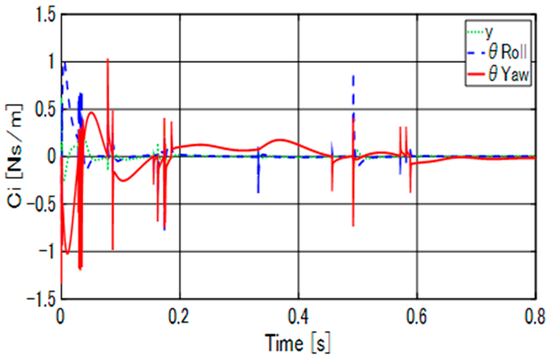
Figure 17 shows the dynamic $C_i$. For the y waveform, oscillations are observed up to 0.2 s. After 0.2 s, although spikes are present, it remains constant at 0 Ns/m. For the ${\theta }_{Roll}$ waveform, it rises to 1 Ns/m immediately after the simulation starts but converges to 0 Ns/m at 0.1 s. After 0.1 s, spikes are visible, but it remains constant at 0 Ns/m. The ${\theta }_{Yaw}$ waveform oscillates and exhibits noticeable spikes, but it reaches 0 Ns/m at 0.8 s and converges to 0 Ns/m.

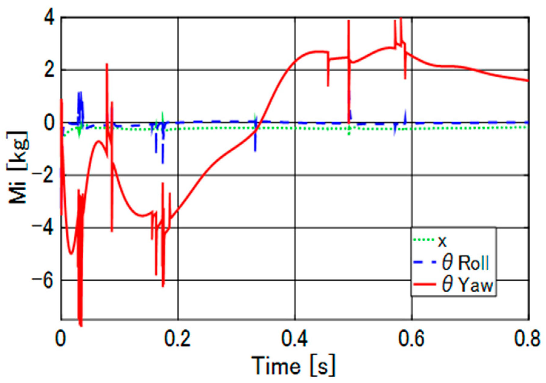
Figure 18 shows the dynamic $M_i$. Regarding the x waveform, it remains constant at approximately −0.4 kg. Regarding the ${\theta }_{Roll}$ waveform, spikes are visible, but it remains constant at approximately 0 kg. Regarding the ${\theta }_{Yaw}$ waveform, it oscillates with negative values from 0 s to 0.35 s and then oscillates with positive values after 0.35 s, showing a decreasing trend after 0.7 s.

6.2. Results When Experimental Conditions Were Changed

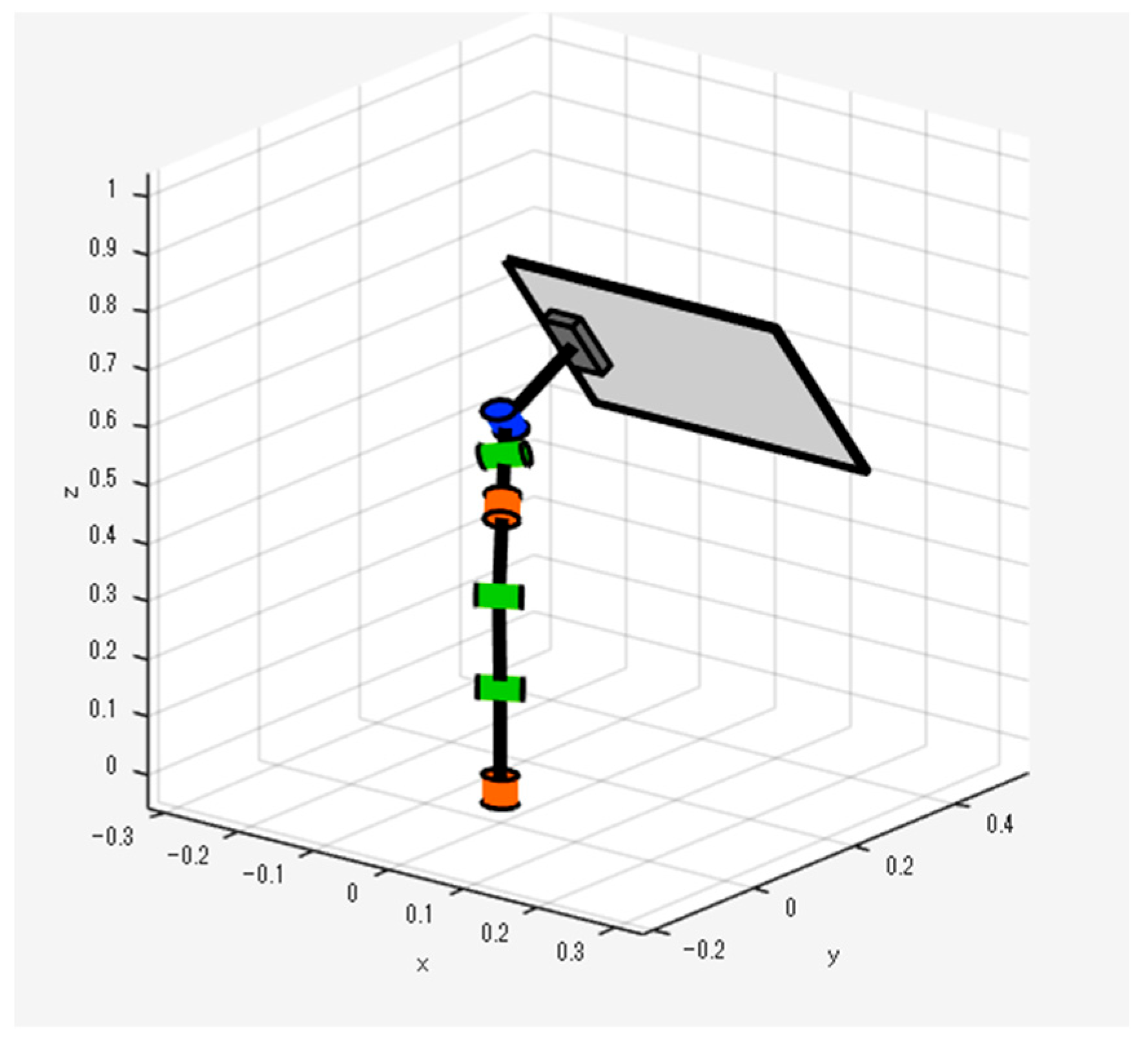
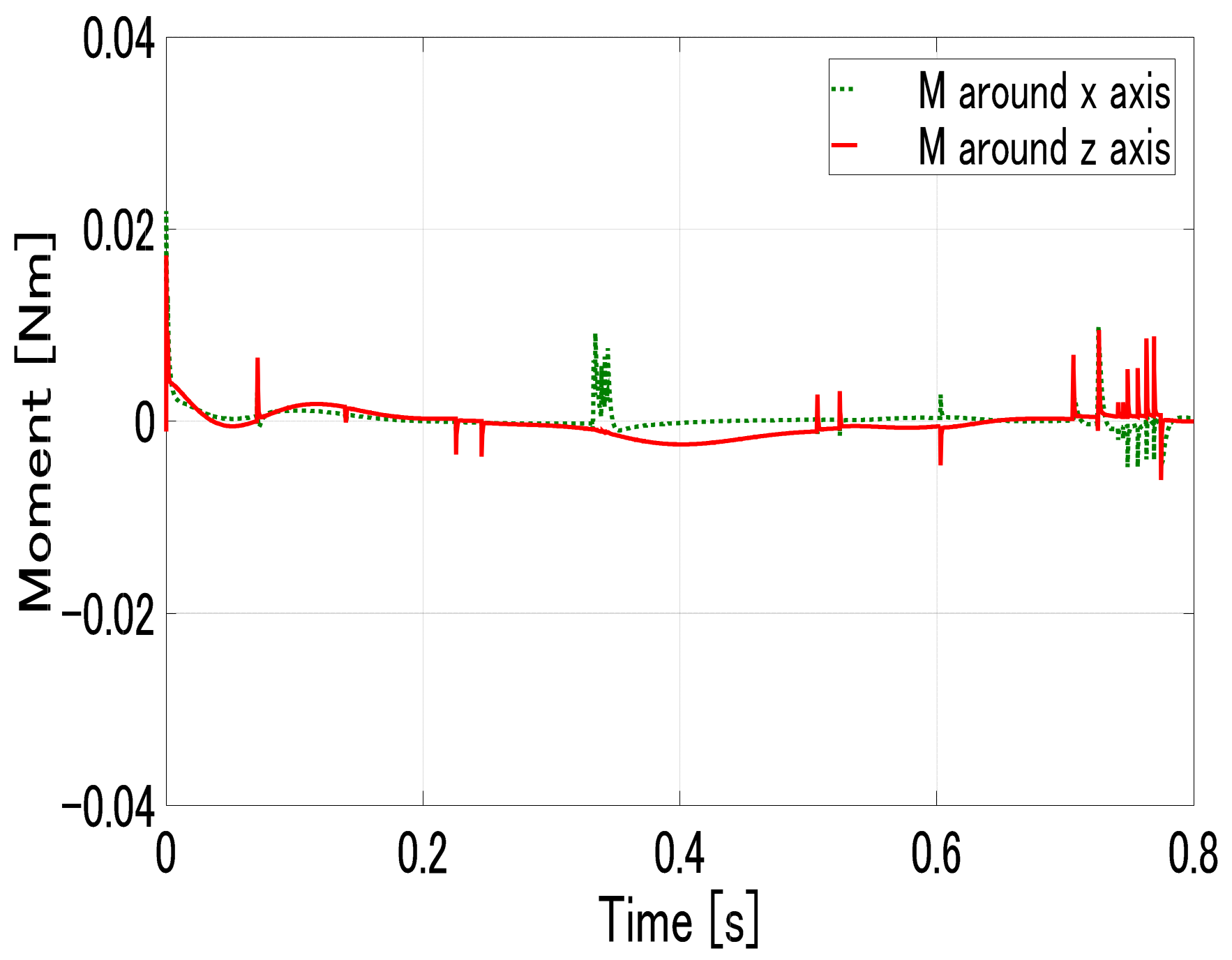
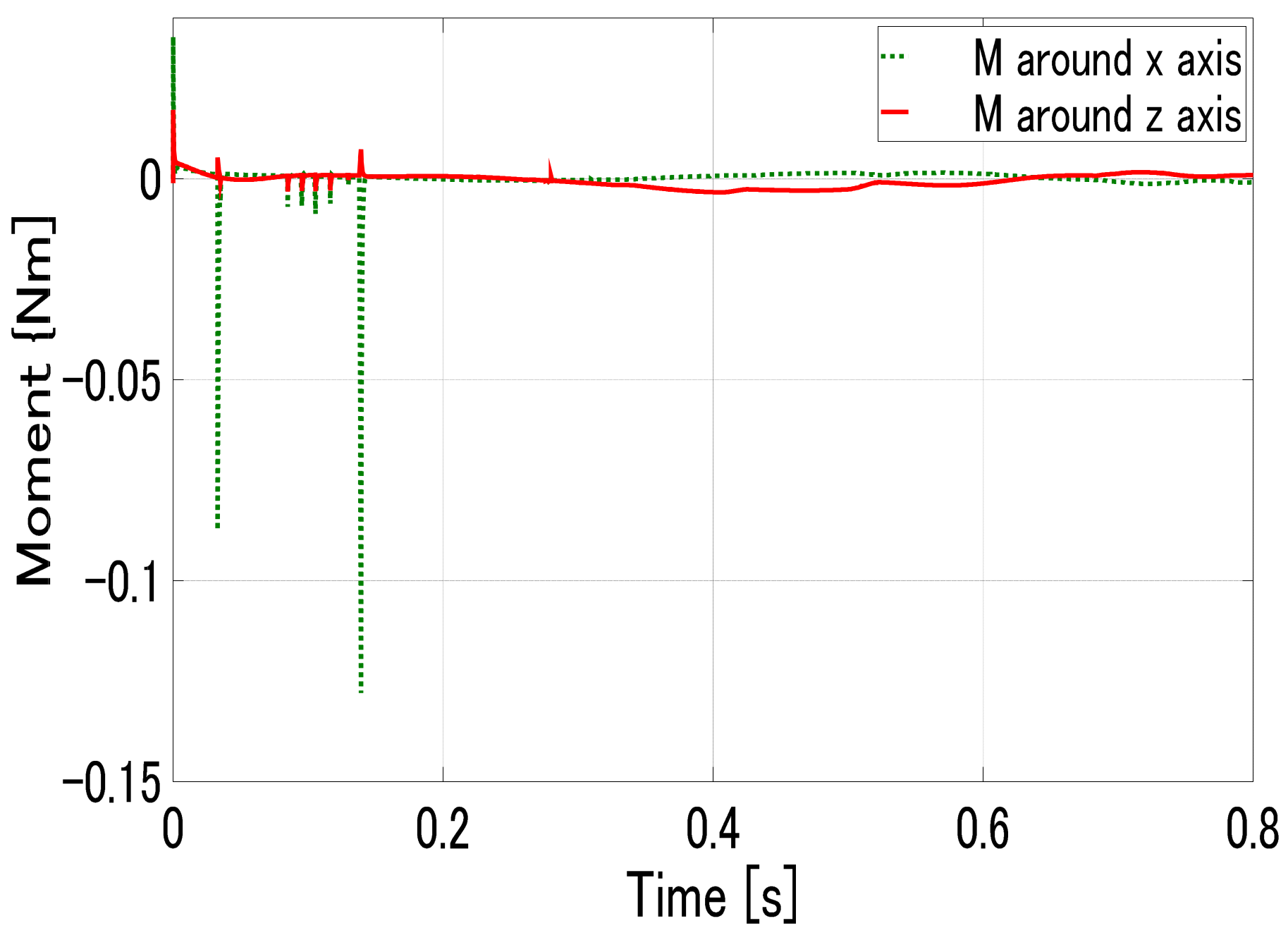
Figure 19 Shows three-dimensional model of a wall at a 30° angle. Figure 20 and Figure 21 showcase where the wall is inclined at a 30° angle, and Figure 19 is a 3D model of the wall in a 30° inclined state. Figure 22 and Figure 23 show the results when the wall’s stiffness is varied by 5%, and Figure 24 and Figure 25 show the results when a disturbance occurs. The disturbance is assumed to have a frequency of 1 Hz and an amplitude of 0.05 m.

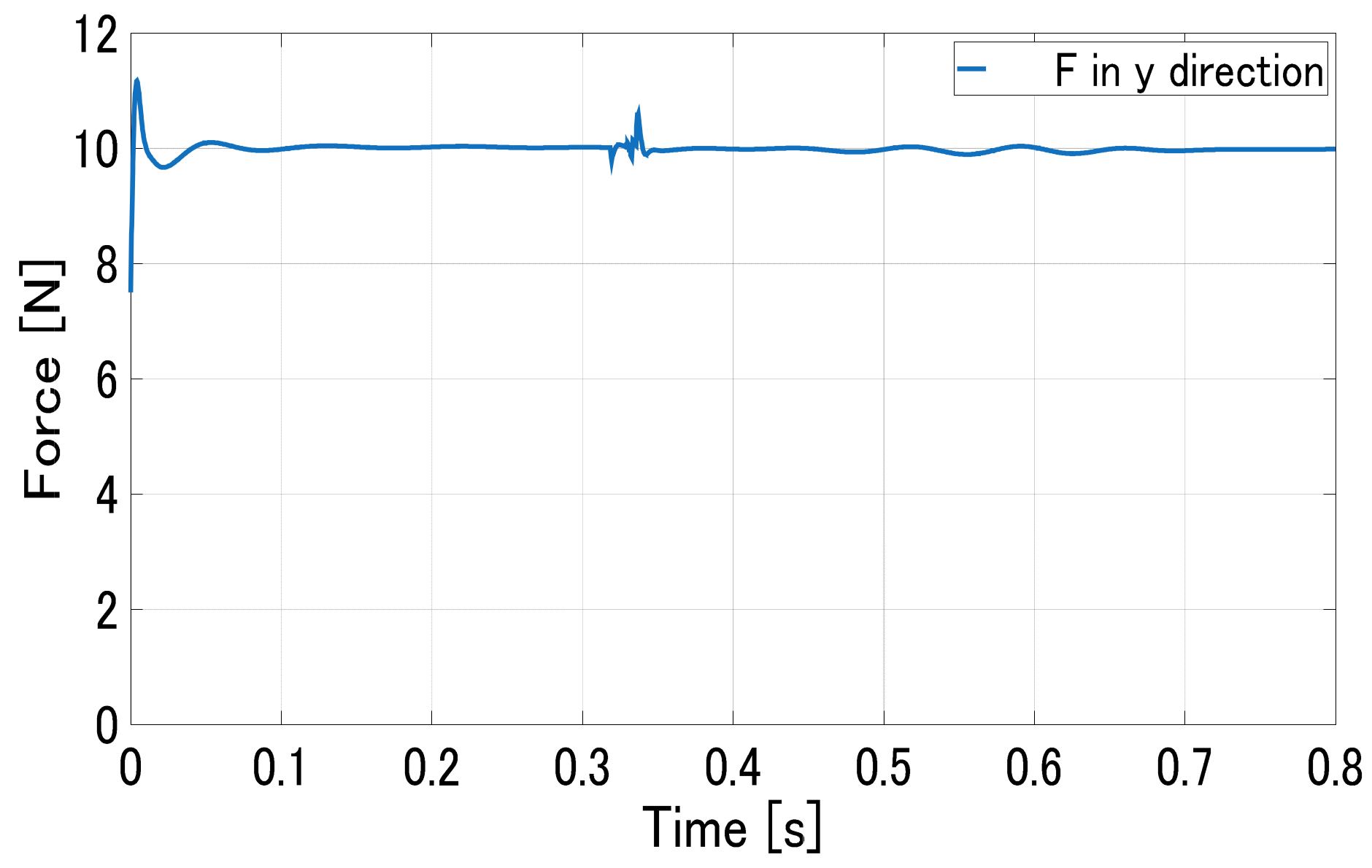
Figure 20 shows the force waveform in the y-direction when a robot with dynamic impedance adaptation is operating on an inclined wall. Observing the waveform, a spike of approximately 11 N occurs at the start of the simulation. Additionally, a spike of approximately 10.5 N is observed at 0.6 s. However, the waveform stabilizes at 10 N, and excluding the spikes, the maximum error relative to the target value is 1% at the 0.5 s mark.

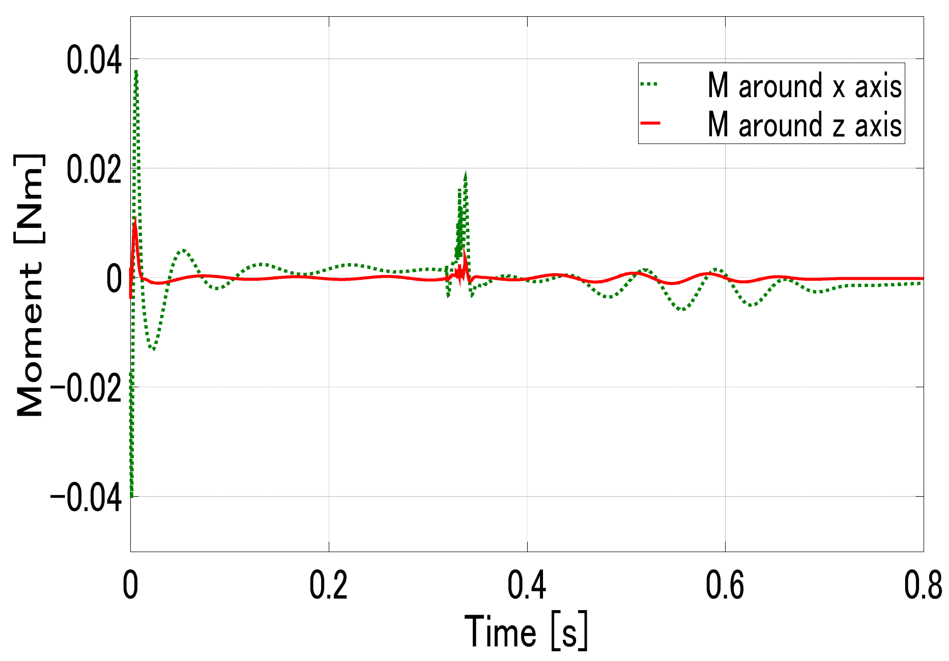
Figure 21 shows the moment waveforms in the $M_x around x axis$ and $M_z around z axis$ when the robot performs tasks against an inclined wall after applying dynamic impedance. Looking at the waveform for the $M_x around x axis$, a spike occurs at the start of the simulation, rising to 0.04 [Nm]. Another spike occurs at 0.33 s, reaching 0.018 [Nm]. The maximum error relative to the target value, excluding the spikes, is −0.0058 [Nm]. Looking at the $M_z around z axis$, a spike also rises at the start of the simulation, reaching 0.009 [Nm]. Furthermore, similar to the $M_x around x axis$, a spike occurs at 0.3 s, reaching 0.0036 [Nm]. However, the $M_z around z axis$ is essentially stable at 0 [Nm], and the maximum error, excluding the spikes, is 0.0007 [Nm].

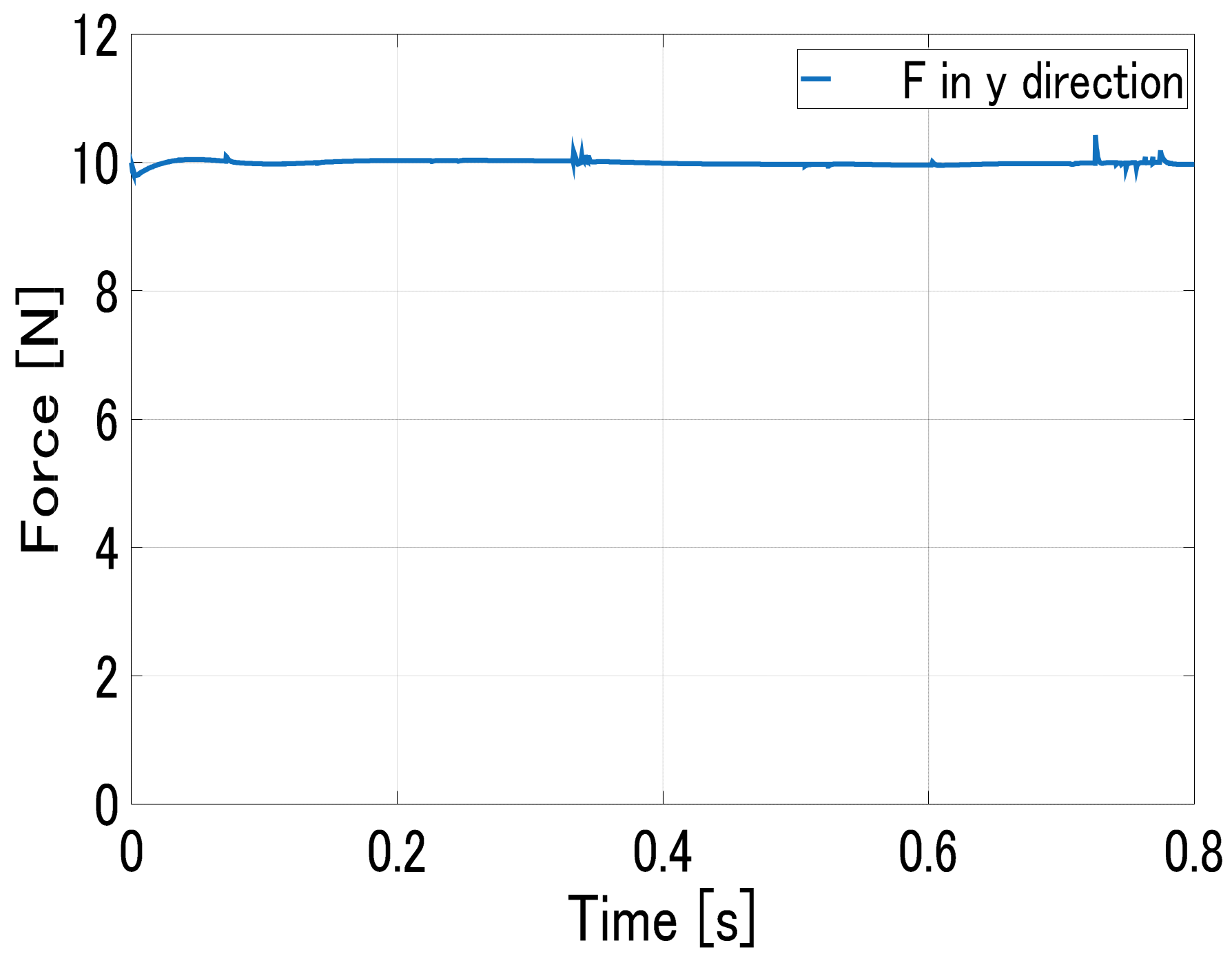
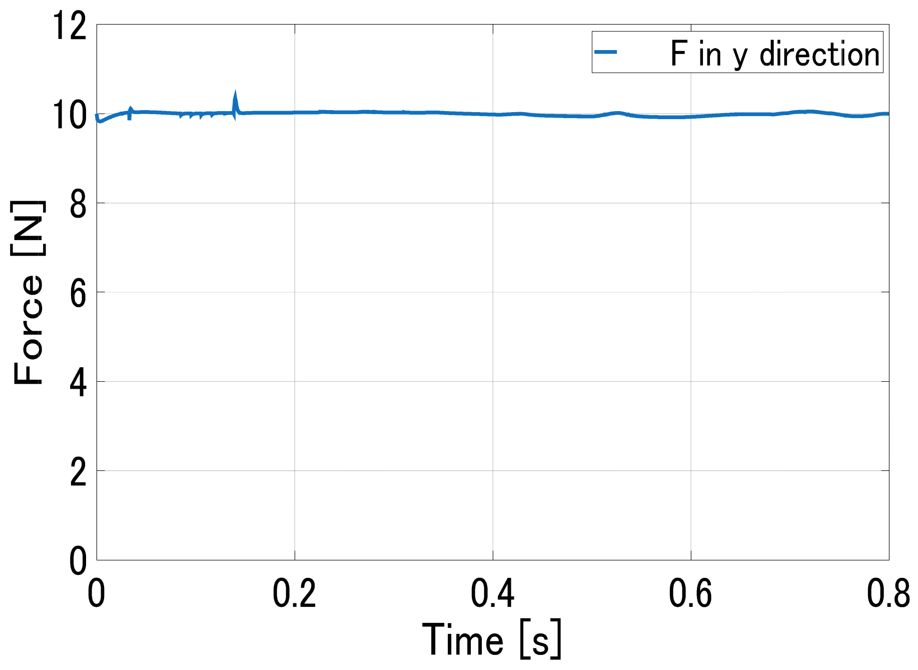
Figure 22 shows the force waveform in the y-direction when the stiffness is increased by 5%. As can be seen here, the system stabilizes at 10 N. Peaks are observed at 0.1 s and 0.73 s. The spike at 0.73 s is 4%.

Figure 23 shows the moment waveforms when the stiffness is increased by 5%. As can be seen here, both the $M_x around x axis$ and the $M_z around z axis$ exhibit waveforms with spikes, with the largest spikes occurring particularly at the start of the simulation. For the $M_x around x axis$, a spike of 0.009 Nm is observed at 0.3 s. For the $M_z around z axis$, a spike of up to 0.008 Nm. occurs; however, both waveforms can be said to be essentially stable at 0 Nm.

Figure 23 shows the force waveform in the y-direction when the wall surface is vibrating. At 0.14 s, a maximum error of 3.5% is observed. As can be seen from this figure, the force waveform remains stable at 10 N.

Figure 24 shows the moment when the waveform occurs as the wall is vibrating. In the waveform labeled the $M_x around x axis$, a large spike reaching −0.12 Nm occurs at 0.14 s. A spike labeled $M_z around z axis$ also occurs at the same time, but its magnitude is small at 0.007 Nm. Although a large spike is observed, it can be seen that the moment waveform is stable at 0 Nm.

Analysis results for the position, posture, force, and moment of the robot arm showed that values after applying dynamic impedance were closer to the simulation target values compared to before its application. This confirmed the effectiveness of dynamic impedance.

7. Conclusions

This study addressed the issue that in the hybrid control of a multi-joint robot using impedance characteristics proposed in a prior study, robustness was insufficient because the impedance characteristics, namely inertia, viscosity, and stiffness, were designed as fixed values. To simultaneously achieve stability, high precision, and robustness, we proposed a hybrid control of a 6-DOF robot arm using dynamic impedance.

Specifically, an impedance model representing virtual inertia, viscosity, and stiffness was designed for the end-effector of the multi-joint robot. This model formalized the equilibrium relationship between the minute displacement and applied force between the end-effector and the contacted workpiece. Next, for the axes undergoing force control, the desired contact force required for the robot end-effector’s minute displacement was added to the target position based on the formulated equilibrium relationship, and position control was performed. For axes not undergoing force control, position control was performed without changing the target position. This approach effectively made both axes position controlled, achieving both stability margin and high precision simultaneously. Furthermore, based on the dynamization of design impedance stiffness based on the final value theorem for steady-state error and the dynamization of design impedance viscosity and inertia based on second-order-form transient response, the relationships between the impedance characteristics, namely inertia, viscosity, and stiffness, and the robot’s joint angles and angular velocities were clarified. This enabled the design of dynamic impedance, simultaneously achieving stability, high precision, and robustness.

To demonstrate the effectiveness of the proposed method, a simulation model of a wall-wiping motion was created for an RPY-type 6-DOF robot arm using mechanism analysis software Inventor (2025 version) and control design software MATLAB/Simulink (2025 version). The simulation results verified its stability, high precision, and robustness.

Future challenges include dynamic wall tracking, adapting to complex objects like spheres for wiping operations, and parameter optimization by using machine learning techniques.

References

1. Raibert, M.H.; Craig, J.J. Hybrid position/force control of robot manipulators. J. Dyn. Syst. Meas. Control 1981, 102, 126–133. [Google Scholar] [CrossRef]
2. Hogan, N. Impedance control: An approach to manipulation: Parts I–III. J. Dyn. Syst. Meas. Control 1985, 107, 1–24. [Google Scholar] [CrossRef]
3. Nguyen, T.H.; Gwak, K.W. Fuzzy adaptive impedance control for the two-layered vertical cable-driven parallel robot. Control Eng. Pract. 2024, 153, 106–110. [Google Scholar] [CrossRef]
4. Kong, H.; Peng, G.; Li, G.; Yang, C. Neural-network-based Optimal Impedance Control for Robots in Physical Interaction With Soft Environments. IEEE Trans. Syst. Man Cybern. Syst. 2025, 55, 6463–6475. [Google Scholar] [CrossRef]
5. Sayyed Noorani, M.R.; Hossein Abud, E.; Sahmani, S.; Safaie, B. Variable impedance models including fuzzy fractional order for control of human–robot interaction: A systematic review. Int. J. Adv. Manuf. Technol. 2025, 139, 4269–4314. [Google Scholar] [CrossRef]
6. Li, L.; Wang, F.; Tang, H.; Liang, Y. Variable-parameter impedance control of manipulator based on RBFNN and gradient descent. Sensors 2025, 25, 49. [Google Scholar] [CrossRef]
7. Carbone, G.; Iannone, S.; Ceccarelli, M. Regulation and control of LARM Hand III, Rob. Robot. Comput.-Integr. Manuf. 2010, 26, 202–211. [Google Scholar] [CrossRef]
8. Lu, Y.; Chang, Z.; Lu, Y.; Wang, Y. Development and kinematics/statics analysis of rigid-flexible-soft hybrid finger mechanism with standard force sensor. Robot. Comput. Integr. Manuf. 2021, 67, 101978. [Google Scholar] [CrossRef]
9. Hadi, A.; Alipour, K.; Kazeminasab, S.; Elahinia, M. ASR glove: A wearable glove for hand assistance and rehabilitation using shape memory alloys. J. Intell. Mater. Syst. Struct. 2018, 29, 1575–1585. [Google Scholar] [CrossRef]
10. Colbaugh, R.; Seraji, H.; Glass, K. Direct adaptive impedance control of robot manipulators. J. Robot. Syst. 1993, 10, 217–248. [Google Scholar] [CrossRef]
11. Khatib, O. A unified approach for motion and force control of robot manipulators: The operational space formulation. IEEE J. Robot. Autom. 1987, 3, 43–53. [Google Scholar] [CrossRef]
12. De Schutter, J.; Van Brussel, H. Compliant robot motion II: A control approach based on external control loops. Int. J. Robot. Res. 1988, 7, 18–33. [Google Scholar] [CrossRef]
13. Abu-Dakka, F.J.; Saveriano, M. Variable impedance control and learning—A review. Front. Robot. AI 2020, 7, 590681. [Google Scholar] [CrossRef]
14. Buchli, J.; Theodorou, E.; Stulp, F.; Schaal, S. Variable impedance control—A reinforcement learning approach. In Robotics: Science and Systems VI; Matsuoka, Y., Durrant-Whyte, H., Neira, J., Eds.; MIT Press: Cambridge, MA, USA, 2011. [Google Scholar] [CrossRef]
15. De Schutter, J.; Van Brussel, H. Compliant robot motion I: A formalism for specifying compliant motion tasks. Int. J. Robot. Res. 1988, 7, 3–17. [Google Scholar] [CrossRef]
16. Bonitz, R.G.; Hsia, T.C. Internal force-based impedance control for cooperating manipulators. IEEE Trans. Robot. Autom. 1996, 12, 78–89. [Google Scholar] [CrossRef]
17. Heck, D.; Saccon, A.; van de Wouw, N.; Nijmeijer, H. Guaranteeing stable tracking of hybrid position–force trajectories for a robot manipulator interacting with a stiff environment. Automatica 2016, 63, 235–247. [Google Scholar] [CrossRef]
18. Zhu, Y.; Liu, C.; Yuan, P.; Li, D. Active impedance control based adaptive locomotion for a bionic hexapod robot. J. Field Robot. 2025, 42, 327–345. [Google Scholar] [CrossRef]
19. Chen, Z.; Zhan, G.; Jiang, Z.; Zhang, W.; Rao, Z.; Wang, H.; Li, J. Adaptive impedance control for docking robot via Stewart parallel mechanism. ISA Trans. 2024, 155, 361–372. [Google Scholar] [CrossRef] [PubMed]
20. Duan, J.; Zhang, K.; Qian, K.; Hao, J.; Zhang, Z.; Shi, C. An operating stiffness controller for the medical continuum robot based on impedance control. Cyborg Bionic Syst. 2024, 5, 0110. [Google Scholar] [CrossRef]
21. Fu, J.; Burzo, I.; Iovene, E.; Zhao, J.; Ferrigno, G.; De Momi, E. Optimization-based variable impedance control of robotic manipulator for medical contact tasks. IEEE Trans. Med. Robot. Bionics 2024, 73, 4004608. [Google Scholar] [CrossRef]
22. Xu, P.; Li, Z.; Liu, X.; Zhao, T.; Zhang, L.; Zhao, Y. Reinforcement learning-based distributed impedance control of robots for compliant operation in tight interaction tasks. Eng. Appl. Artif. Intell. 2024, 136, 108913. [Google Scholar] [CrossRef]
23. Zhang, Y.; Li, T.; Tao, H.; Liu, F.; Hu, B.; Wu, M.; Yu, H. Research on Adaptive Impedance Control Technology of Upper Limb Rehabilitation Robot Based on Impedance Parameter Prediction. Front. Bioeng. Biotechnol. 2024, 11, 1332689. [Google Scholar] [CrossRef] [PubMed]
24. Huang, Q.; Saito, K.; Nonami, K. Position and posture, force and moment hybrid control for hand of 6-DOF manipulator. In Symposium on Motion and Vibration Control; Japan Society of Mechanical Engineers: Tokyo, Japan, 2005; Volume 9, pp. 481–486, (In Japanese). [Google Scholar] [CrossRef]
25. Huang, Q.; Enomoto, R. Position/posture/force/moment hybrid control of 6-DOF manipulator: Realization of the arbitrary direction and verification with the RPY type machine. In Symposium on Motion and Vibration Control; Japan Society of Mechanical Engineers: Tokyo, Japan, 2007; Volume 9, pp. 322–327, (In Japanese). [Google Scholar] [CrossRef]
26. Whitney, D.E. Resolved Motion Rate Control of Manipulators and Human Prostheses. IEEE Trans. Man-Mach. Syst. 1969, 10, 47–53. [Google Scholar] [CrossRef]
Figure 1. PUMA type.
Robotics 15 00074 g001
Figure 2. RPY type.
Robotics 15 00074 g002
Figure 3. Iterative search method.
Robotics 15 00074 g003
Figure 4. Hybrid control of position, posture, force, and moment via differential inverse kinematics.
Robotics 15 00074 g004
Figure 5. Joint coordinate system.
Robotics 15 00074 g005
Figure 6. Center of mass.
Robotics 15 00074 g006
Figure 7. Dynamic model.
Robotics 15 00074 g007
Figure 8. MATLAB/Simulink simulation model of the RPY-type 6-DOF robot arm.
Robotics 15 00074 g008
Figure 9. Contact point [12].
Robotics 15 00074 g009
Figure 10. Parameter definition.
Robotics 15 00074 g010
Figure 11. Schematic of wall-wiping task and end-effector coordinate frame.
Robotics 15 00074 g011
Figure 12. Comparison of positions before and after dynamic impedance adaptation.
Robotics 15 00074 g012
Figure 13. Comparison of posture before and after applying dynamic impedance.
Robotics 15 00074 g013
Figure 14. Comparison of force before and after applying dynamic impedance.
Robotics 15 00074 g014
Figure 15. Comparison of moments before and after applying dynamic impedance.
Robotics 15 00074 g015
Figure 16. Dynamized K i .
Robotics 15 00074 g016
Figure 17. Dynamized C i .
Robotics 15 00074 g017
Figure 18. Dynamized M i .
Robotics 15 00074 g018
Figure 19. Three-dimensional model of a wall at a 30° angle.
Robotics 15 00074 g019
Figure 20. Force waveform at a 30° angle to the wall.
Robotics 15 00074 g020
Figure 21. Waveform of the moment at a 30° wall angle.
Robotics 15 00074 g021
Figure 22. Force waveform when stiffness is increased by 5%.
Robotics 15 00074 g022
Figure 23. Moment waveform when stiffness is increased by 5%.
Robotics 15 00074 g023
Figure 24. Force waveform when the wall is vibrating.
Robotics 15 00074 g024
Figure 25. Waveform of the moment when the wall is vibrating.
Robotics 15 00074 g025