Integrated Design of a Modular Lower-Limb Rehabilitation Exoskeleton: Multibody Simulation, Load-Driven Structural Optimization, and Experimental Validation ^†

Abstract

Lower-limb rehabilitation exoskeletons must balance biomechanical compatibility, structural safety, and low mass to enable practical, repeatable gait assistance. This paper proposes a planar pantograph-derived exoskeleton leg driven by a Chebyshev Lambda linkage and develops an integrated workflow from mechanism synthesis to manufacturable optimization and experimental verification. A mannequin-coupled multibody model was built in MSC ADAMS to evaluate joint kinematics, end-point (foot) trajectories, and joint reaction forces under multiple scenarios (fixed-frame, ramp, stair ascent, and inclined-plane walking). The extracted joint loads were transferred to a parametric finite element model in ANSYS Workbench 2019, where response surface surrogates and a multi-objective genetic algorithm (MOGA) were used to minimize mass under stiffness and strength constraints. For the optimized load-bearing link, the selected minimum-mass design reached a component mass of 0.542 kg while respecting the imposed structural limits, i.e., a maximum total deformation below 0.2 mm and a maximum equivalent (von Mises) stress below 50 MPa (e.g., ~0.188 mm deformation and ~39 MPa stress in the optimal candidate). A rapid prototype was manufactured by 3D printing and experimentally evaluated using CONTEMPLAS high-speed video tracking, providing measured X_M(t) and Y_M(t) trajectories and joint-angle histories for quantitative comparison with simulations via RMSE metrics.

1. Introduction

1.1. State of the Art on Lower-Limb Rehabilitation Exoskeleton Robotic Systems

Lower-limb rehabilitation exoskeletons have become a major research and development direction due to the growing need for intensive, repeatable gait therapy in neurological and musculoskeletal conditions. Recent reviews emphasize that the field is no longer limited by proof-of-concept feasibility, but by persistent barriers to clinical translation: safe physical human–robot interaction, user variability (anthropometry, impairment level, spasticity, fatigue), energy autonomy, comfort and donning/doffing time, affordability, and the lack of standardized performance metrics and benchmarking across platforms [1,2]. In parallel, systematic surveys focused on locomotion-assistance exoskeletons highlight that reproducibility and transparent reporting (mechanical, sensing, and control specifications) remain inconsistent, making cross-comparisons and evidence synthesis difficult [3].

1.2. Mechanical Design Trends and Biomechanical Compatibility

A core theme in the recent literature is that exoskeleton performance cannot be judged only by actuator torque or tracking accuracy; it must be evaluated in terms of biomechanical compatibility and the quality of interaction at the hip, knee, and ankle. Foundational biomechanical guidelines stress joint-axis alignment, kinematic compatibility, mass distribution, and avoidance of parasitic constraints to reduce discomfort and undesired joint loading. These principles remain central in modern design frameworks, especially for rehabilitation devices where users often exhibit altered gait patterns and limited tolerance to misalignment [4].

At the opposite end of the spectrum, soft wearable robots and exosuits are increasingly studied for their comfort and low mass. A detailed review of soft wearable robots summarizes dominant actuation approaches (e.g., cable-driven and fluidic systems), fabrication trends, and typical application domains, while also pointing out ongoing challenges in force transmission efficiency, durability, and repeatable assistance delivery [5]. Within this landscape, compliant and semi-compliant solutions have gained attention as a means to improve safety and reduce sensitivity to joint misalignment. A comprehensive review on compliant lower-limb exoskeletons consolidates mechanical design principles such as elastic elements and compliant transmissions, while discussing the trade-offs between interaction safety and control precision [6].

Recent advances in soft wearable robotics further highlight the importance of lightweight, compliant, and body-conformable actuation concepts. Lu et al. [7,8] reported a fully flexible wearable pouch pneumatic artificial muscle based on asymmetric expansion, designed to reduce wear-side compression while maintaining high contraction performance. Cho et al. proposed a bidirectional double-spring pneumatic artificial muscle with inductive self-sensing, showing how lightweight wearable actuators can integrate both actuation and sensing functions. Although the present study focuses on a rigid pantograph-derived rehabilitation mechanism rather than a soft exosuit, these contributions are relevant because they emphasize comfort, compliance, and sensing integration as important design directions for future wearable assistive robots.

Actuation technology continues to shape practical deployment. A recent scoping review on lower-limb exoskeleton actuation provides a structured view of motors, reducers, and reporting gaps, and explicitly calls for standardized disclosure of actuator characteristics to enable meaningful reproducibility and comparison. This push toward more complete technical reporting aligns with broader survey observations that device-level details often remain underreported despite being critical for interpretability and transferability [9].

1.3. Control Strategies, Intention Recognition, and Learning-Based Methods

Control is widely recognized as the enabling layer for safe and adaptive assistance. Recent reviews dedicated to exoskeleton control strategies describe the diversity of approaches, including trajectory tracking, impedance/admittance control, assist-as-needed paradigms, and methods driven by intention estimation, while also emphasizing the need for unified evaluation criteria and clinically meaningful outcome measures [10].

A notable trend is the integration of motion intention recognition and multi-sensor fusion to personalize assistance. For example, methods combining intention recognition with active control are reported for rehabilitation robots, focusing on improving the responsiveness of assistance to the user’s movement goals [11]. Other approaches fuse multiple sensor sources (e.g., kinematic and interaction signals) to infer intention more robustly and to support adaptive control strategies [12]. Physiological and plantar information are also used to enhance intention detection and gait-phase estimation; exoskeleton/prosthesis approaches incorporating EMG and baropodometric (plantar pressure) measurements exemplify this direction toward multi-modal, user-aware control [13].

Learning-based methods are increasingly explored to improve adaptability, especially when impairment patterns vary across users and across sessions. A representative example is the application of deep reinforcement learning strategies (e.g., TD3/DDPG variants) for motion control in a lower-limb rehabilitation exoskeleton context, reflecting the broader shift toward data-driven adaptation—while also raising practical questions about safety, generalization, and validation in clinical populations [14]. At the same time, fundamental investigations into how robotic torque pulses can entrain gait provide useful insight for designing assistance strategies that exploit neuromechanical dynamics rather than enforcing rigid trajectories; such evidence supports control concepts that are “minimally encumbering” while still shaping gait patterns [15].

Recent research also shows that intelligent control is evolving beyond conventional trajectory tracking toward data-driven modeling of human–robot interaction and biomechanically informed path generation. Khan et al. [16] proposed a quantum-enhanced transformer framework to learn transactive energy during physical human–robot interaction, pointing to new possibilities for interaction-aware assistance control. In a related contribution, reinforcement learning was used to generate ankle-rehabilitation trajectories under musculoskeletal-informed energy optimization, demonstrating that learning-based methods can support personalized motion planning while preserving biomechanical relevance. These studies reinforce the view that future lower-limb exoskeleton development should combine mechanism design, sensing, and adaptive data-driven control [17].

Recent studies also show that data-driven methods can also support mechanism synthesis and personalization at the kinematic-design stage. For example, Khan et al. [18] combined deep learning and optimization to relate sagittal-plane gait trajectories to the dimensions and inverse-kinematics solution of a six-bar rehabilitation mechanism, thereby highlighting the potential of AI-assisted customization. The present study addresses a complementary problem: instead of learning subject-specific mechanism dimensions from gait data, it develops an integrated engineering workflow for a pantograph-derived exoskeleton leg, in which multibody simulation is used to extract joint loads that are subsequently transferred to finite-element-based structural optimization and then checked experimentally on a rapid prototype.

1.4. Sensing Technologies and Measurement-Driven Evaluation

Sensing has evolved from basic joint encoders toward richer multi-modal measurement systems used for control, monitoring, and clinical assessment. A recent comprehensive review focusing on sensor technologies and control strategies for lower-limb rehabilitation exoskeletons highlights the role of IMUs, force/pressure sensing, EMG, and integrated sensing architectures in enabling reliable state estimation and safer assistance modulation. This direction also aligns with device-level studies that explicitly incorporate EMG and plantar measurements for rehabilitation-oriented evaluation and adaptive behavior. Together, these contributions reinforce the idea that robust exoskeleton assistance requires both mechanical integrity and measurement-informed control [19].

1.5. Clinical Evidence in Stroke, SCI, and Pediatric Rehabilitation

Clinical translation is increasingly supported by randomized trials and meta-analyses, but evidence remains heterogeneous due to variability in devices, protocols, and patient populations. For stroke rehabilitation, recent randomized and pilot randomized clinical trials investigate exoskeleton-assisted gait training outcomes in subacute populations, including unilateral configurations and specific balance/gait end-points [20,21]. A randomized controlled trial targeting non-ambulatory subacute stroke patients evaluates an exoskeleton-based physical therapy program within inpatient rehabilitation, reflecting a pragmatic approach to integrating exoskeleton sessions into standard care pathways [22]. Another randomized study incorporating the Hybrid Assistive Limb (HAL) into subacute stroke gait training provides additional evidence regarding feasibility and clinical integration for patients with severe walking limitations [23].

At the evidence-synthesis level, meta-analyses and systematic reviews address the effects of wearable exoskeleton interventions on post-stroke gait rehabilitation, aggregating available trial data and identifying both benefits and methodological limitations across studies [24]. Similarly, a systematic review on wearable lower-limb exoskeletons for gait training in neuromuscular impairments supports broader conclusions about suitability, constraints, and the need for careful patient selection and protocol design [25].

For spinal cord injury (SCI), multiple reviews and meta-analyses evaluate exoskeleton-assisted gait training with respect to gait ability, balance, and motor function, often comparing exoskeleton-based interventions with conventional therapies and reporting substantial heterogeneity in outcomes and protocols. This body of evidence underscores the importance of standardized outcome measures and transparent reporting of training dosage, assistance mode, and patient inclusion criteria [26,27,28].

Beyond adult populations, pediatric rehabilitation is also expanding, as demonstrated by a randomized clinical trial investigating a soft robotic exoskeleton to improve lower-limb motor function in children with spastic cerebral palsy—highlighting additional constraints on safety, mass, fit, and long-term comfort. Together, these clinical studies emphasize that successful deployment depends not only on performance but also on usability, tolerability, and protocol integration across clinical settings [29].

1.6. Consolidated Gaps and Research Opportunities

Across the recent literature, several recurring gaps motivate ongoing research. First, despite advances in design and control, there remains a disconnect between engineering metrics (torque, tracking error, stress margins) and clinical/functional outcomes (walking independence, balance, endurance), complicating device comparison and optimization [1,2,3,4,5,6,7,8,9,10,11,12,13,14,15,16,17,18,19,20,21,22,23,24,25,26,27,28]. Second, reproducibility is limited by incomplete reporting of actuation specifications, control parameters, and sensor configurations; recent surveys and scoping reviews explicitly call for standardization to enable meaningful cross-study comparison. Third, while adaptive control and learning-based approaches are promising, their safe translation requires careful validation and robust intention-estimation pipelines—particularly for impaired gait and variable assistance needs. Finally, biomechanical compatibility remains central: alignment, compliance, and interaction quality at hip/knee/ankle are repeatedly identified as determinants of comfort and safety, reinforcing the need for biomechanically grounded mechanisms and validated interaction models [29].

In this context, system-level implementations that integrate robust actuation and hybrid control remain important reference points for practical device development [30]. Overall, the state of the art suggests that future progress will be driven by integrated workflows combining biomechanically informed design, measurement-driven adaptive control, and reproducible reporting—supported by clinical evidence and standardized evaluation protocols.

In response to this gap, this paper presents:

○

A planar linkage-based lower-limb exoskeleton mechanism, developed from kinematic synthesis to a manufacturable CAD assembly suitable for rapid prototyping.

○

A coupled multibody dynamic simulation in MSC ADAMS using a human mannequin with aligned hip, knee, and ankle joints and an impact-based ground-contact model to capture gait-relevant interaction loads.

○

Extraction of joint reaction forces from the multibody model to define representative loading conditions for structural assessment.

○

A parametric FE-based structural optimization in ANSYS using response surfaces and MOGA to obtain a minimum-mass manufacturable design under stress/deformation constraints.

The proposed system is intended as a mechanism-level lower-limb rehabilitation prototype for adult users performing therapist-supervised gait training in the sagittal plane, rather than as an unsupervised daily-use exoskeleton. Accordingly, the design requirements adopted in this study were defined at the level of nominal fitting and motion assumptions: gait-relevant hip flexion/extension, knee flexion sufficient to reproduce the clearance phase, adjustment of the main leg dimensions to the intended user anthropometry, and nominal alignment of the exoskeleton hip and knee joints with the corresponding anatomical joint centers before simulation and testing. In the present paper, these requirements are treated as engineering design inputs for mechanism synthesis, multibody simulation, and prototype evaluation, not yet as clinically validated fitting limits.

The present manuscript is an extended and substantially revised version of our conference contribution “Development of a New Leg Mechanism for Exoskeleton Robots: Structural Synthesis, Dynamic Analysis, and Prototype Implementation”, presented at the International Workshop IFToMM for Sustainable Development Goals (I4SDG 2025) and subsequently selected for possible inclusion in the associated Robotics Special Issue [31].

2. Structural Solutions for Exoskeleton Legs Based on a Pantograph Mechanism

Two alternative structural solutions were developed for the exoskeleton leg. Both rely on a planar pantograph-type closed kinematic chain, but they differ in the input linkage used to drive the pantograph mechanism. Each pantograph solution comprises seven kinematic links interconnected through fourteen revolute joints, enabling sagittal-plane assistance of the lower limb while maintaining a compact, lightweight architecture. The two designs share the same pantograph core, but they differ in the input structural group that drives the pantograph, which leads to distinct motion transmission characteristics and load paths.

2.1. Solution I: Pantograph Leg Driven by an Articulated Quadrilateral Input Linkage

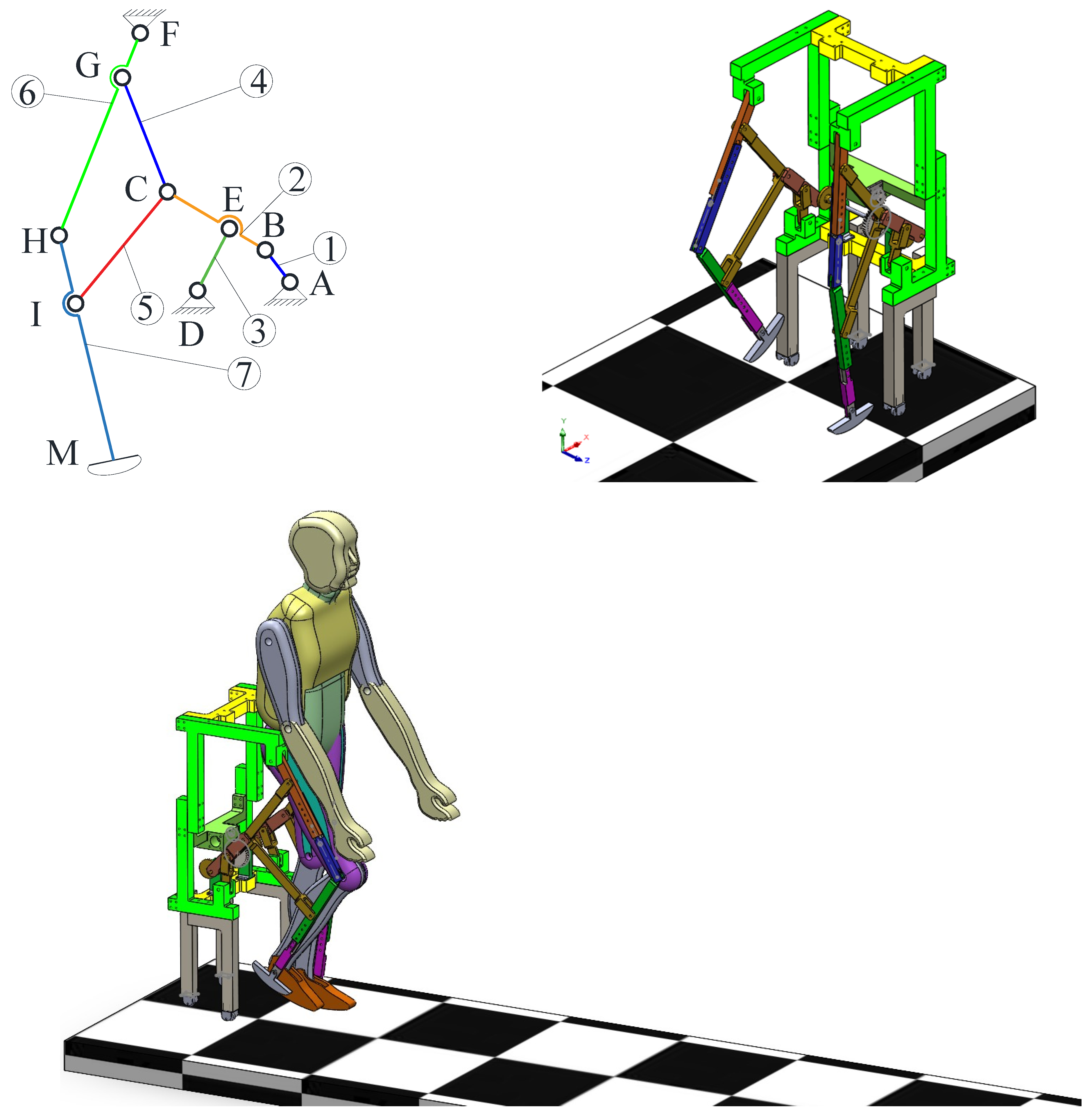
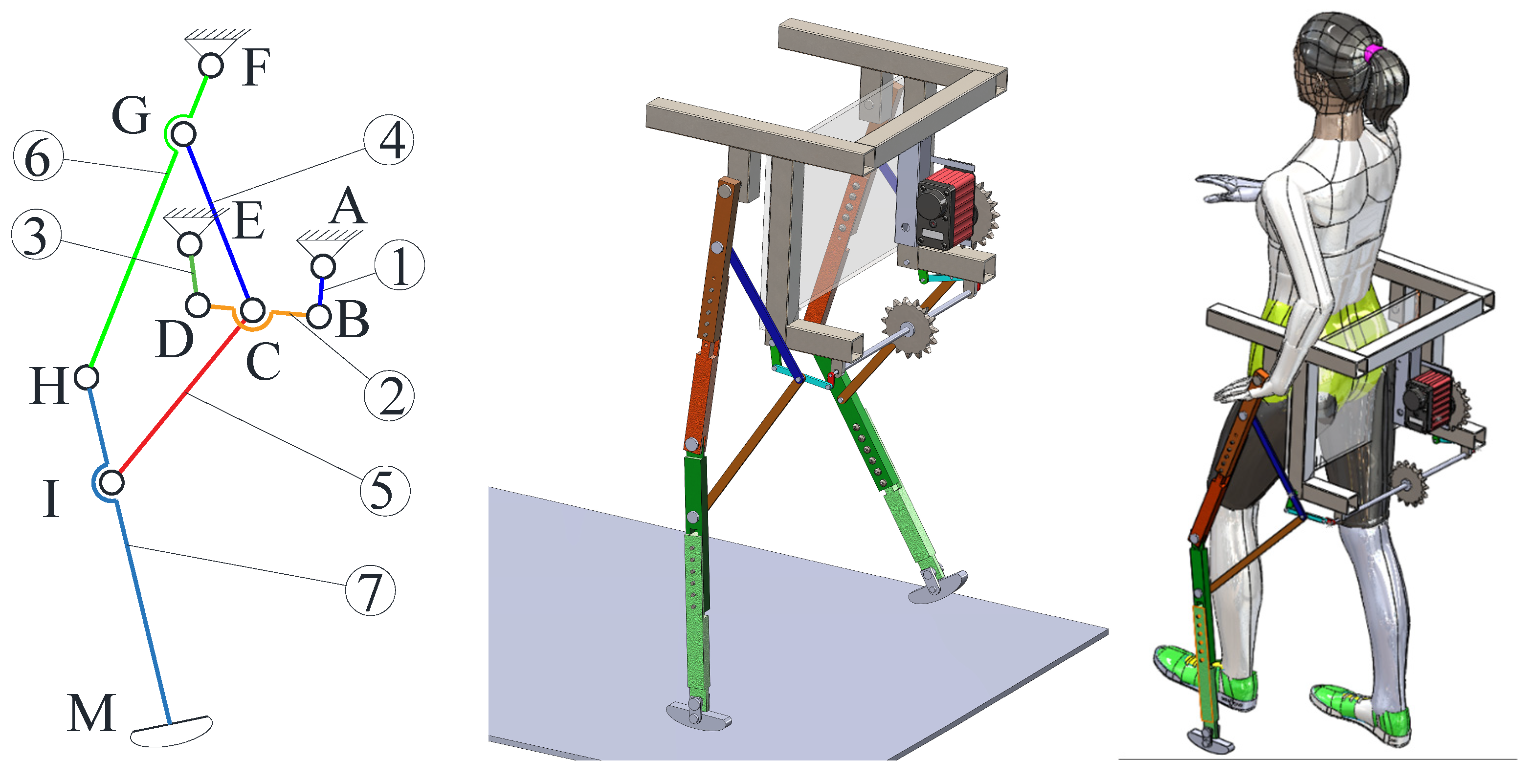
The first solution (Figure 1) employs three RRR dyad structural groups (BDE, CGF, and CIH), while the pantograph core is formed by links (4)–(7). In this configuration, link (6) is associated with the femur segment and link (7) with the tibia segment, whereas joint F represents the hip joint and joint H represents the knee joint. Motion is transmitted to the pantograph by coupling joint C to link (2) of an articulated quadrilateral (four-bar) input mechanism, which acts as the driver of the entire leg structure [32].

A corresponding virtual prototype was developed to verify manufacturability and assembly feasibility. The model includes a lightweight frame, a gear-driven actuation arrangement, and a chain transmission visible at the prototype level, while the waist support ensures stable attachment to the user and preserves alignment between the exoskeleton and the hip–knee anatomical joints in the virtual mannequin representation.

In the planar kinematic scheme (left), the letters denote the characteristic points and revolute joints of the mechanism. Points A, E, and F are fixed joints attached to the supporting frame, while B, C, D, G, H, and I are moving joint centers. Point M denotes the distal foot/contact point of the exoskeleton leg. The circled numbers identify the main links of the mechanism: 1—input link AB, 2—link B–C–D, 3—link E–D, 4—link C–G, 5—link C–I, 6—link F–G–H, and 7—distal link H–I–M. The different colored lines are used only to distinguish the individual kinematic members and to facilitate their visual correspondence with the 3D CAD model and the mannequin-coupled representation.

In the middle image, the mechanism is shown as a 3D CAD assembly integrated into the supporting frame, where the colored members correspond to the links indicated in the planar scheme. In the right image, the same exoskeleton concept is shown coupled with a human mannequin, highlighting the relative placement of the device with respect to the human lower limb. The gray base surface represents the ground/support plane, while the transparent mannequin is included to illustrate the intended wearable configuration.

2.2. Solution II: Pantograph Leg Driven by a Chebyshev Lambda Mechanism

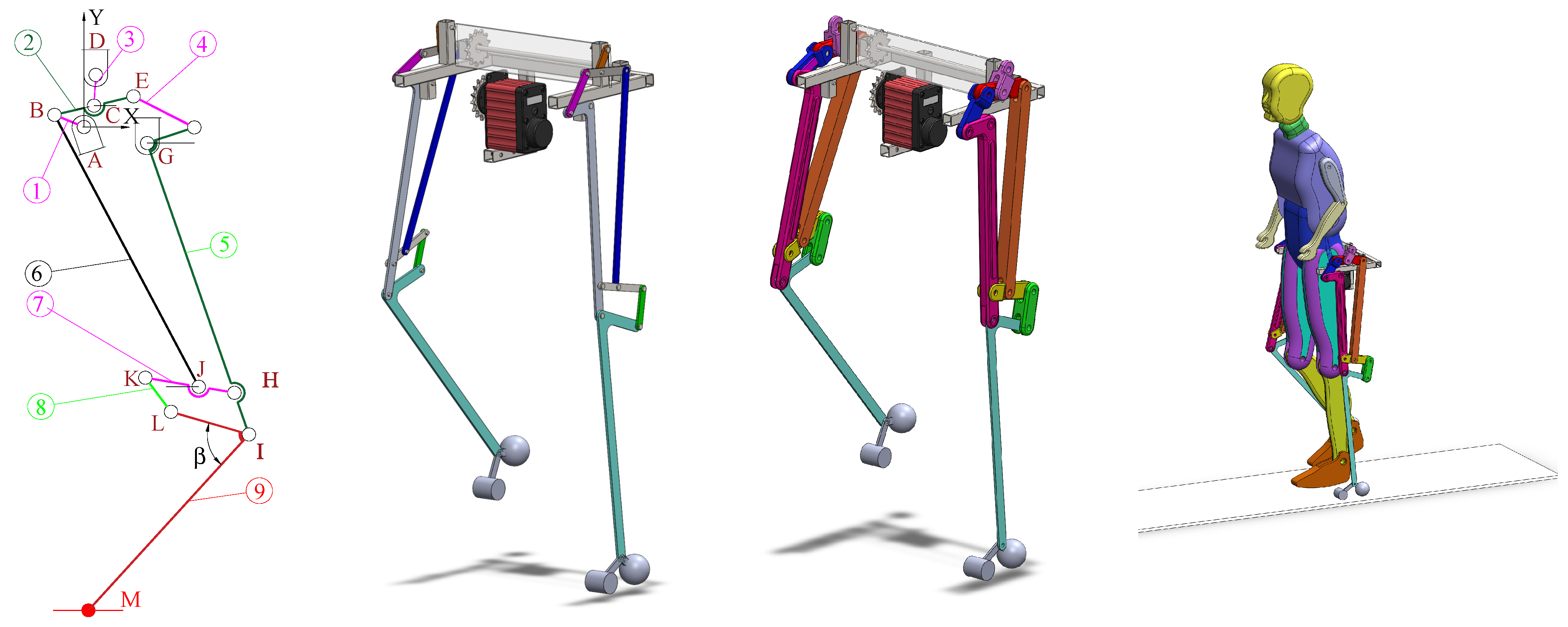
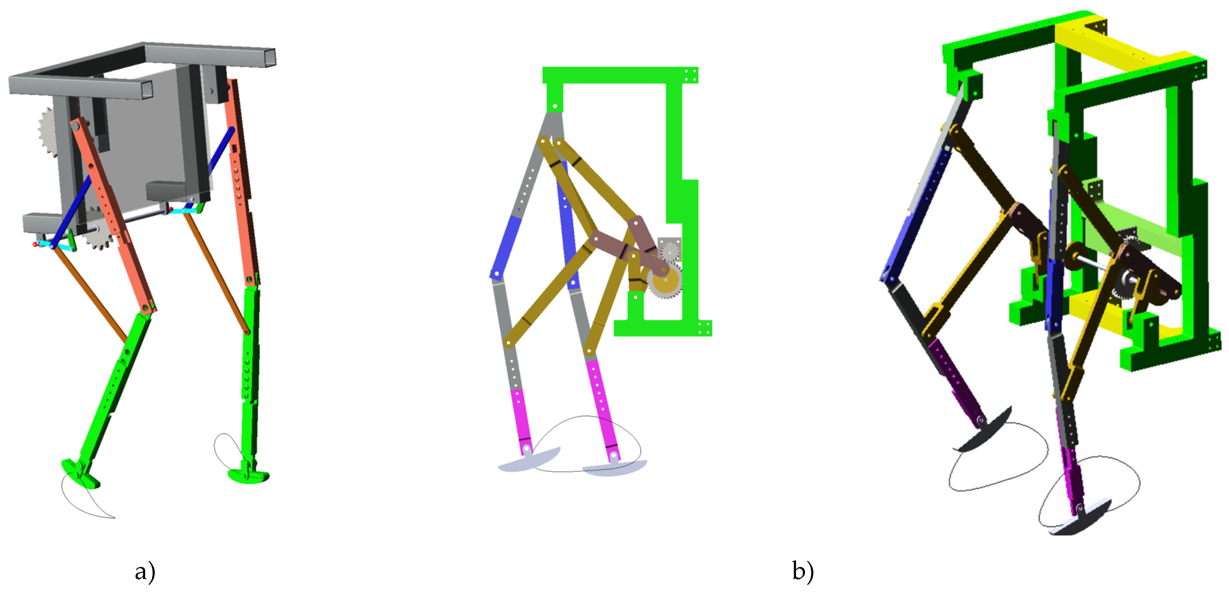
The second solution (Figure 2) retains the pantograph core (links (4)–(7)) but replaces the input structural group with a Chebyshev Lambda kinematic chain, which drives the pantograph through a gear-based transmission. The pantograph remains a symmetric linkage intended to reproduce femur–tibia coordinated motion, with joint F assigned to the hip and joint H assigned to the knee. Compared to Solution I, the Chebyshev Lambda input chain provides an alternative motion-generation architecture that can improve gait-like trajectory generation and overall kinematic behavior.

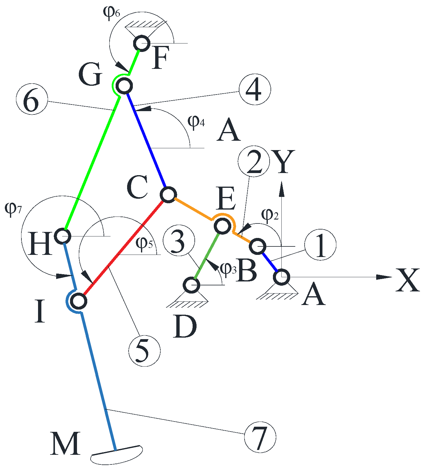
In the left-hand side of the figure, the letters denote the characteristic points of the planar kinematic scheme. Points A, D, and F are the fixed attachment points to the supporting frame, while B, C, E, G, H, and I are moving revolute joint centers. Point M denotes the distal point of the mechanism, associated with the foot/end-effector trajectory. The circled numbers identify the kinematic links of the mechanism: 1—link AB, 2—ternary link B–E–C, 3—link D–E, 4—link C–G, 5—link I–C, 6—link H–G–F, and 7—distal link H—I–M. The different colored lines are used to distinguish the individual links in the kinematic diagram and to make their correspondence with the 3D CAD representation easier to follow. The hatched symbols at points A, D, and F indicate grounded joints.

In the right-hand side of the figure, the same mechanism is shown as a 3D CAD assembly. The green and yellow parts represent the main supporting frame, while the colored moving members correspond to the links highlighted in the planar scheme. The gray lower parts represent the foot/end-contact elements, and the black-and-white surface represents the ground plane.

At system level, the virtual prototype for Solution II incorporates a reinforced frame for improved structural stability while maintaining low mass, and places the actuation in a central position to support balanced weight distribution. The architecture is modular, allowing geometric adjustments consistent with the user’s anthropometric data, and the pantograph elements are intended to be further refined through finite-element-based optimization to reduce mass while preserving stiffness.

In addition to the two pantograph-based alternatives, the leg architecture can be interpreted as a self-contained mechanism derived from the 2024 patent [33], on a modular lower-limb exoskeleton, as shown in Figure 3. In the kinematic scheme, the letters A–M denote the 13 kinematic joints (pairs), while the numbers 1–9 identify the 9 kinematic elements (links) of the mechanism. Point M denotes the characteristic distal point of the mechanism. It is built around a four-bar (articulated quadrilateral) driving group, complemented by auxiliary links that shape the distal trajectory. Rather than being derived from a pantograph layout, the implemented solution uses the quadrilateral as the primary motion-generating unit, which transmits the input to the remaining loops and directly governs the coordination between the hip and knee rotations. The auxiliary links are introduced to refine the end-point behavior and obtain the desired ovoid foot path while preserving compactness and modularity. This quadrilateral-centered architecture provides a clear synthesis framework and a controllable set of design parameters, which is advantageous for CAD implementation, multibody simulation, and subsequent load-driven structural optimization.

2.3. Comparative Note and Selection Rationale

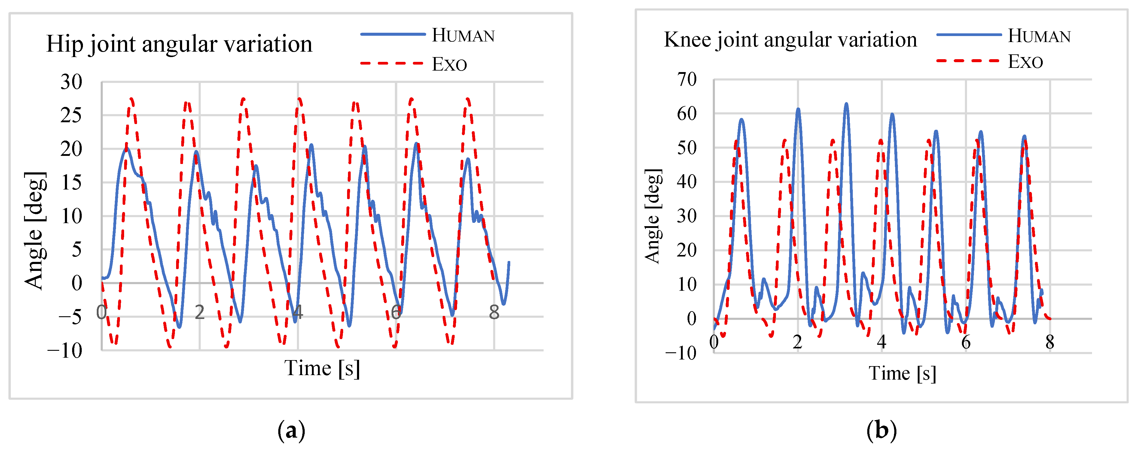
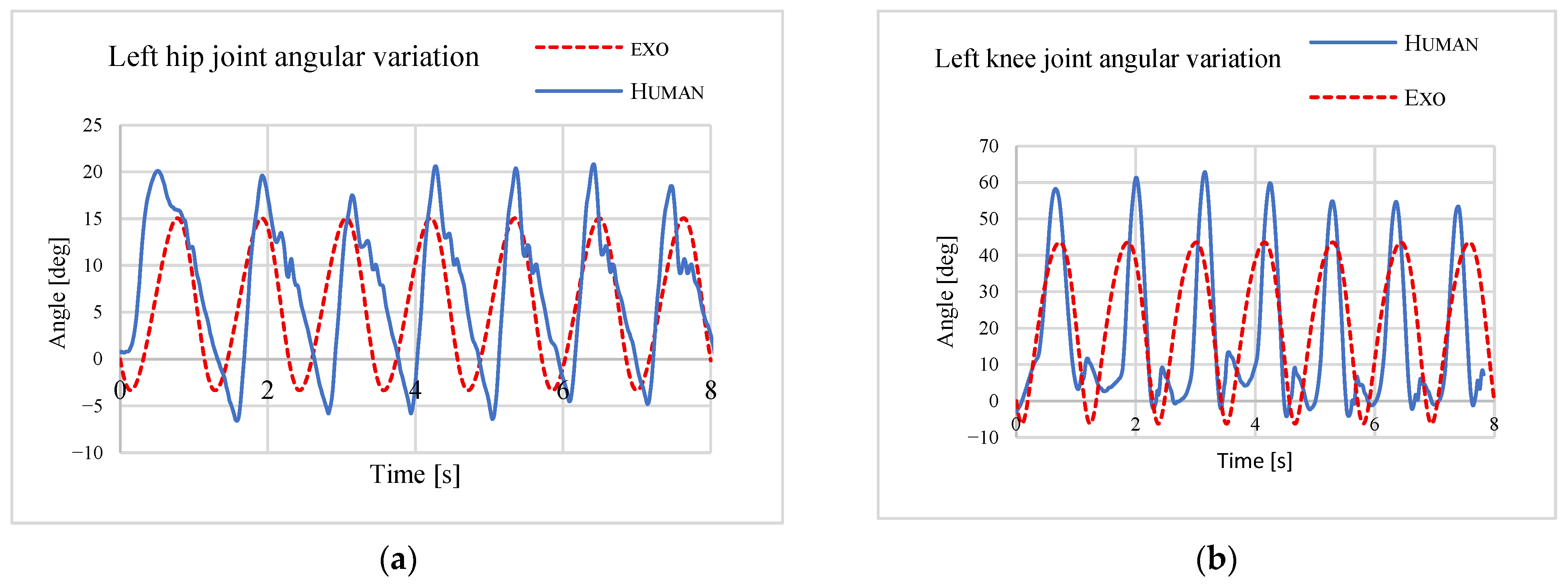
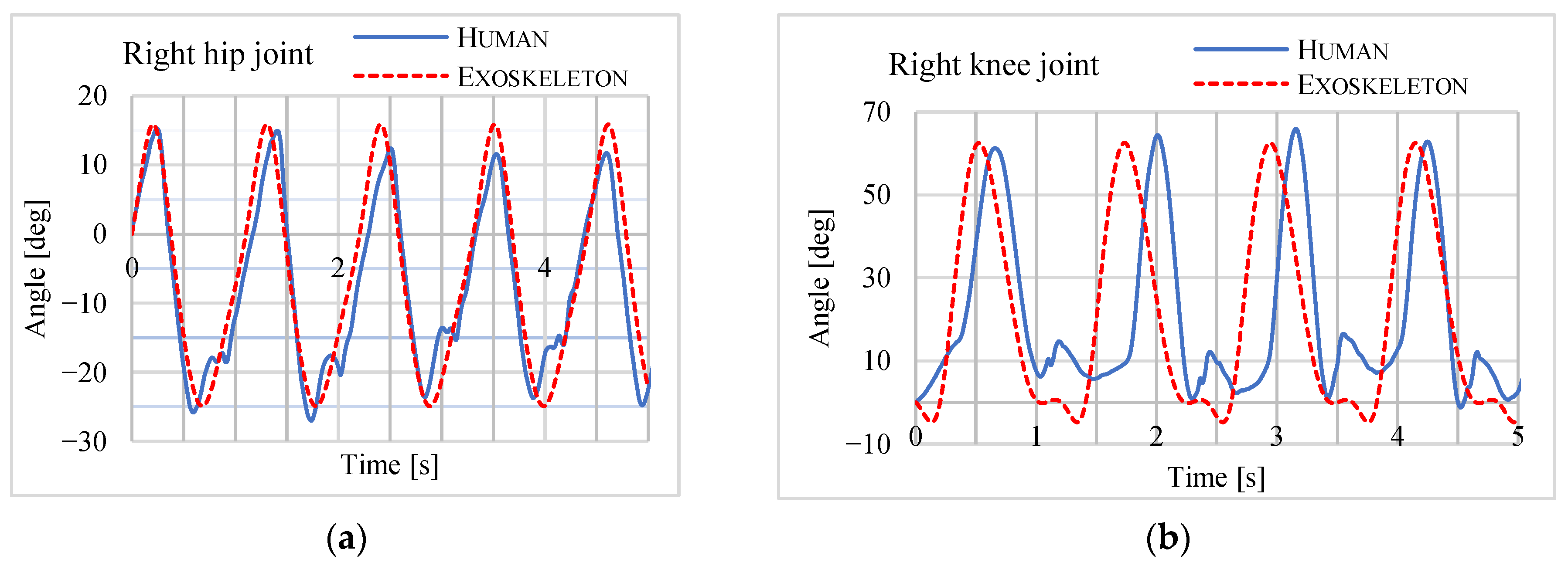
Although the three candidate leg mechanisms share the same general objective of generating gait-like sagittal-plane motion, their kinematic outputs differ significantly because of the distinct input structural groups and motion-transmission layouts. Therefore, the comparative assessment was extended beyond a qualitative inspection of the foot-path shape (Figure 4a,b) and also included the evolution of the hip and knee joint angles obtained from the ADAMS exoskeleton–mannequin simulations, compared against a healthy human gait reference (Figure 5, Figure 6 and Figure 7).

As shown in the comparative plots, the three solutions do not reproduce the hip–knee coordination with the same degree of similarity to the reference gait pattern. In particular, the comparison was based on the overall shape of the angular histories, the relative timing between hip and knee flexion/extension, the smoothness of the profiles over the gait-like cycle, and the consistency between joint-angle evolution and the generated end-point trajectory. These indicators were considered more informative than the sole visual appearance of the foot path, because they better reflect the mechanism’s ability to reproduce physiologically plausible sagittal-plane coordination.

Among the investigated configurations, Solution II, based on the Chebyshev Lambda driving mechanism, provided the most suitable overall kinematic behavior for the purpose of the present study. In comparison with the other solutions, it generated smoother joint-angle profiles, a more coherent phase relationship between hip and knee motion, and a gait-like end-point progression compatible with the intended mechanism-level rehabilitation scenario. In addition, this configuration offered a more convenient arrangement of the drive and supporting frame, which facilitated its subsequent implementation in the integrated multibody simulation, structural optimization, and prototype-validation workflow.

The selection of Solution II was therefore not based solely on the ovoid shape of the sole trajectory, but on a combined kinematic and implementation-oriented assessment. At the same time, this choice should be interpreted as a preliminary engineering selection within the scope of the present mechanism-level study, rather than as a definitive ranking with respect to all wearable-exoskeleton performance criteria. Metrics such as backdrivability, reflected inertia, stance-phase torque efficiency, interaction-force sensitivity, and tolerance to joint misalignment were not separately quantified here and remain important topics for future investigation.

Nevertheless, the remainder of this paper focuses on Solution II, which was adopted as the reference architecture for the subsequent ADAMS dynamic analyses, ANSYS structural optimization, and prototype-level experimental validation.

3. Kinematic Model Validation for Gait-like Trajectory Generation and Optimal Structural Design

In this subsection, an analytical kinematic model of the selected leg mechanism is developed as the foundation for kinematic evaluation and subsequent synthesis/optimization. The mechanism is modeled as a planar multi-loop linkage (Figure 5), fully parameterized by the fixed joint coordinates and the link dimensions defined in the kinematic scheme. The resulting formulation yields explicit position relationships for the main joints and for the distal point M as functions of the driving input, enabling systematic assessment of end-effector motion, hip–knee coordination, and admissible joint ranges.

Beyond validating gait-relevant behavior, the analytical model is essential for tailoring the mechanism to different users. Because the exoskeleton is conceived as a modular structure with adjustable-length elements—particularly the links representing the femur and tibia—its geometry must be re-synthesized for different anthropometric dimensions while preserving biomechanical alignment and target joint excursions. The parametric kinematic equations provide a direct way to update link lengths, enforce kinematic constraints, and define objective functions (e.g., ovoid sole-path quality, clearance, and joint-range targets) for optimizing the mechanism across subject-specific anthropometry. This ensures that physiologically plausible trajectories are obtained before proceeding to mannequin-coupled dynamic simulation and structural optimization.

User-specific adaptation is performed through a parametric resizing procedure. First, the target anthropometric quantities of the intended user are defined, primarily the thigh length, shank length, and the corresponding hip–knee and knee–ankle reference distances. Next, the exoskeleton links associated with the femur-like and tibia-like segments are resized so that the exoskeleton joint spacing matches the target limb dimensions while preserving the topology of the pantograph-derived mechanism. The fixed joint locations and driving-link dimensions are then re-synthesized using the analytical kinematic model, and the updated configuration is re-checked in MSC ADAMS to verify that the desired gait-like trajectory, joint excursions, and load levels are maintained. Therefore, in the present study, anthropometric adaptation is addressed as a modular parametric design procedure rather than as a finalized automatic adjustment subsystem.

A similar closed-loop leg mechanism has been reported by Li and Ceccarelli for a rickshaw/biped prototype [34,35]; however, the architecture developed in this work is distinct in that the main leg linkage is actuated through a Chebyshev Lambda driving mechanism, which imposes the input motion and shapes the gait-oriented end-point trajectory via a dedicated powertrain rather than a direct four-bar excitation.

As can be seen from the kinematic scheme shown in Figure 8, the structural solution comprises 7 kinematic elements connected by 14 rotational joints. So, the exoskeleton robot solution provides assistance only for the flexion/extension movements of the human leg, realized in the sagittal plane. In the kinematic scheme, the letters A–M denote the 10 kinematic joints (pairs), while the numbers 1–7 identify the 7 kinematic elements (links) of the mechanism. Point M denotes the characteristic distal point of the mechanism. The different colors distinguish the kinematic members and their correspondence with the 3D representations.

A theoretical analysis of the leg exoskeleton kinematics was performed in order to evaluate and simulate performances and operation. The point M position, reported to the XY reference system, Figure 8, is evaluated as a function of input angle φ₁ and dimensional parameters of the linkage. Geometrical parameters are presented in

Table 1. Geometrical parameters used in the analytical kinematic model.

Category	Parameter	Value (Units)
Fixed joint coordinates	A	xA = 0 mm; yA = 0 mm
Fixed joint coordinates	D	xD = −73.5 mm; yD = −42 mm
Fixed joint coordinates	F	xF = −270 mm; yF = 421 mm
Link lengths	lAB	25 mm
Link lengths	lBE	80 mm
Link lengths	lDE	100 mm
Link lengths	lBC	180 mm
Link lengths	lFG	90 mm
Link lengths	lGC	270 mm
Link lengths	lCI	330 mm
Link lengths	lFH	430 mm
Link lengths	lHI	430 mm
Link lengths	lIM	260 mm
Input motion	ω1	2 rad/s (constant angular velocity of link 1)

.

It is considered an angular velocity of link (1) equal to 2 rad/s. The coordinates of joint B are computed with Equation (1).

$${\displaystyle \frac{\mathrm{d}{\mathsf{\phi }}_1}{\mathrm{d}\mathrm{t}}}={\mathsf{\omega }}_1\Rightarrow {\mathsf{\phi }}_1={\mathsf{\omega }}_1·\mathrm{t}; {\mathsf{\omega }}_1=2\mathrm{r}\mathrm{a}\mathrm{d}/\mathrm{s}$$

$$\left\{\begin{array}{c}{\mathrm{x}}_{\mathrm{B}}={\mathrm{x}}_{\mathrm{A}}+{\mathrm{l}}_{\mathrm{A}\mathrm{B}}\cdot \cos {\mathsf{\phi }}_1\\ {\mathrm{y}}_{\mathrm{B}}={\mathrm{y}}_{\mathrm{A}}+{\mathrm{l}}_{\mathrm{A}\mathrm{B}}\cdot \sin {\mathsf{\phi }}_1\end{array}\right.$$

(1)

3.1. Dyad BED Kinematics (Assur Structural Group)

The joint E coordinates are obtained from the loop-closure equations:

$$\left\{\begin{array}{c}{\mathrm{x}}_{\mathrm{E}}={\mathrm{x}}_{\mathrm{B}}+{\mathrm{l}}_{\mathrm{B}\mathrm{E}}\cdot \cos {\mathsf{\phi }}_2={\mathrm{x}}_{\mathrm{D}}+{\mathrm{l}}_{\mathrm{D}\mathrm{E}}\cdot \cos {\mathsf{\phi }}_3\\ {\mathrm{y}}_{\mathrm{E}}={\mathrm{y}}_{\mathrm{B}}+{\mathrm{l}}_{\mathrm{B}\mathrm{E}}\cdot \sin {\mathsf{\phi }}_2={\mathrm{y}}_{\mathrm{D}}+{\mathrm{l}}_{\mathrm{D}\mathrm{E}}\cdot \sin {\mathsf{\phi }}_3\end{array}\right.$$

(2)

To compute angle φ₃, the unknown φ₂ is eliminated by grouping terms and then squaring and summing. Using the notations $\left(x_D-x_B\right)=a_1$; and $\left(y_D-y_B\right)=a_2$, the resulting trigonometric equation is:

$$\left\{\begin{array}{c}{l}_{BE}\cdot \mathit{cos}{\phi }_2=\left(x_D-x_B\right)+l_{DE}\cdot \mathit{cos}{\phi }_3\\ l_{BE}\cdot \mathit{sin}{\phi }_2=\left(y_D-y_B\right)+l_{DE}\cdot \mathit{sin}{\phi }_3\end{array}\right.$$

(3)

Equations of system (3) after square and summing becomes:

$${\mathrm{a}}_1^2+{\mathrm{a}2}_2+{{\mathrm{l}}_{\mathrm{B}\mathrm{E}}}^2-{\mathrm{l}}_{\mathrm{D}\mathrm{E}}^2-2{\mathrm{a}}_1{\mathrm{l}}_{\mathrm{D}\mathrm{E}}\cos {\mathsf{\phi }}_3-2{\mathrm{a}}_2{\mathrm{l}}_{\mathrm{D}\mathrm{E}}\sin {\mathsf{\phi }}_3=0$$

(4)

Equation (4) can be written in the standard form:

$$A_3\mathit{sin}{\phi }_3+B_3\mathit{cos}{\phi }_3+C_3=0$$

(5)

The solution is obtained using the tangent half-angle substitution:

$${\mathsf{\phi }}_3=2\mathrm{a}\mathrm{r}\mathrm{c}\mathrm{t}\mathrm{g}{\displaystyle \frac{{\mathrm{A}}_3\pm \sqrt{{\mathrm{A}}_3^2+{\mathrm{B}}_3^2-{\mathrm{C}}_3^2}}{{\mathrm{B}}_3-{\mathrm{C}}_3}}$$

(6)

where ${\mathrm{A}}_3=-2{\mathrm{a}}_2{\mathrm{l}}_{\mathrm{D}\mathrm{E}};{\mathrm{B}}_3=-2{\mathrm{a}}_1{\mathrm{l}}_{\mathrm{D}\mathrm{E}};{\mathrm{C}}_3=-{\mathrm{a}}_1^2-{\mathrm{a}}_2^2+{\mathrm{l}}_{\mathrm{B}\mathrm{E}}^2-{\mathrm{l}}_{\mathrm{D}\mathrm{E}}^2$.

Similarly, by eliminating φ₃, a trigonometric equation in φ₂ is obtained and solved as:

$$\begin{gathered} l_{DE}^2-a_1^2-{a2}_2-{l_{BE}}^2+2a_1{l}_{BE}\mathit{cos}{\phi }_2+2a_2{l}_{BE}\mathit{sin}{\phi }_2=0 \\ {\mathsf{\phi }}_2=2\mathrm{a}\mathrm{r}\mathrm{c}\mathrm{t}\mathrm{g}{\displaystyle \frac{{\mathrm{A}}_2\pm \sqrt{{\mathrm{A}}_2^2+{\mathrm{B}}_2^2-{\mathrm{C}}_2^2}}{{\mathrm{B}}_2-{\mathrm{C}}_2}} \end{gathered}$$

(7)

where ${\mathrm{A}}_2=2{\mathrm{a}}_2{\mathrm{l}}_{\mathrm{B}\mathrm{E}};{\mathrm{B}}_2=2{\mathrm{a}}_1{\mathrm{l}}_{\mathrm{B}\mathrm{E}};{\mathrm{C}}_2={\mathrm{l}}_{\mathrm{D}\mathrm{E}}^2-{\mathrm{a}}_1^2-{\mathrm{a}}_2^2-{\mathrm{l}}_{\mathrm{B}\mathrm{E}}^2$.

The physically consistent branch is selected according to the assembled configuration and motion continuity.

3.2. Assur Structural Group CGF Kinematics

The joint G coordinates are obtained from the loop-closure equations:

$$\begin{array}{c}{\mathrm{x}}_{\mathrm{G}}={\mathrm{x}}_{\mathrm{C}}+{\mathrm{l}}_{\mathrm{C}\mathrm{G}}\cdot \cos {\mathsf{\phi }}_4={\mathrm{x}}_{\mathrm{F}}+{\mathrm{l}}_{\mathrm{F}\mathrm{G}}\cdot \cos {\mathsf{\phi }}_6\\ {\mathrm{y}}_{\mathrm{G}}={\mathrm{y}}_{\mathrm{C}}+{\mathrm{l}}_{\mathrm{C}\mathrm{G}}\cdot \sin {\mathsf{\phi }}_4={\mathrm{y}}_{\mathrm{F}}+{\mathrm{l}}_{\mathrm{F}\mathrm{G}}\cdot \sin {\mathsf{\phi }}_6\end{array}$$

(8)

With $\left({\mathrm{x}}_{\mathrm{C}}-{\mathrm{x}}_{\mathrm{F}}\right)={\mathrm{a}}_3$ and $\left({\mathrm{y}}_{\mathrm{C}}-{\mathrm{y}}_{\mathrm{F}}\right)={\mathrm{a}}_4$, the unknown angles are computed by reducing the loop to the standard form (9).

$$\begin{gathered} {{\mathrm{l}}_{\mathrm{F}\mathrm{G}}}^2-{\mathrm{a}}_3^2-{\mathrm{a}2}_4-{\mathrm{l}}_{\mathrm{C}\mathrm{G}}^2-2{\mathrm{a}}_3{\mathrm{l}}_{\mathrm{C}\mathrm{G}}\cos {\mathsf{\phi }}_4-2{\mathrm{a}}_4{\mathrm{l}}_{\mathrm{C}\mathrm{G}}\sin {\mathsf{\phi }}_4=0 \\ {\mathsf{\phi }}_4=2\mathrm{a}\mathrm{r}\mathrm{c}\mathrm{t}\mathrm{g}{\displaystyle \frac{{\mathrm{A}}_4\pm \sqrt{{\mathrm{A}}_4^2+{\mathrm{B}}_4^2-{\mathrm{C}}_4^2}}{{\mathrm{B}}_4-{\mathrm{C}}_4}} \end{gathered}$$

(9)

where ${\mathrm{A}}_4=-2{\mathrm{a}}_4{\mathrm{l}}_{\mathrm{C}\mathrm{G}};{\mathrm{B}}_4=-2{\mathrm{a}}_3{\mathrm{l}}_{\mathrm{C}\mathrm{G}};{\mathrm{C}}_4={\mathrm{l}}_{\mathrm{F}\mathrm{G}}^2-{\mathrm{a}}_3^2-{\mathrm{a}}_4^2-{\mathrm{l}}_{\mathrm{C}\mathrm{G}}^2$.

Similarly, by eliminating φ₄, a trigonometric equation in φ₆ is obtained and solved as:

$$\begin{gathered} {l_{CG}}^2-a_3^2-{a2}_4-l_{FG}^2+2a_3{l}_{FG}\mathit{cos}{\phi }_6+2a_4{l}_{FG}\mathit{sin}{\phi }_6=0 \\ {\mathsf{\phi }}_6=2\mathrm{a}\mathrm{r}\mathrm{c}\mathrm{t}\mathrm{g}{\displaystyle \frac{{\mathrm{A}}_6\pm \sqrt{{\mathrm{A}}_6^2+{\mathrm{B}}_6^2-{\mathrm{C}}_6^2}}{{\mathrm{B}}_6-{\mathrm{C}}_6}} \end{gathered}$$

(10)

where ${\mathrm{A}}_6=2{\mathrm{a}}_4{\mathrm{l}}_{\mathrm{F}\mathrm{G}};{\mathrm{B}}_6=2{\mathrm{a}}_3{\mathrm{l}}_{\mathrm{F}\mathrm{G}};{\mathrm{C}}_6={\mathrm{l}}_{\mathrm{C}\mathrm{G}}^2-{\mathrm{a}}_3^2-{\mathrm{a}}_4^2-{\mathrm{l}}_{\mathrm{F}\mathrm{G}}^2$.

3.3. Assur Structural Group CIH Kinematics

The joint I coordinates are obtained from the loop-closure equations:

$$\begin{array}{c}{\mathrm{x}}_{\mathrm{I}}={\mathrm{x}}_{\mathrm{H}}+{\mathrm{l}}_{\mathrm{H}\mathrm{I}}\cdot \cos {\mathsf{\phi }}_7={\mathrm{x}}_{\mathrm{C}}+{\mathrm{l}}_{\mathrm{C}\mathrm{I}}\cdot \cos {\mathsf{\phi }}_5\\ {\mathrm{y}}_{\mathrm{I}}={\mathrm{y}}_{\mathrm{H}}+{\mathrm{l}}_{\mathrm{H}\mathrm{I}}\cdot \sin {\mathsf{\phi }}_7={\mathrm{y}}_{\mathrm{C}}+{\mathrm{l}}_{\mathrm{C}\mathrm{I}}\cdot \sin {\mathsf{\phi }}_5\end{array}$$

(11)

With $\left({\mathrm{x}}_{\mathrm{C}}-{\mathrm{x}}_{\mathrm{H}}\right)={\mathrm{a}}_5$ and $\left({\mathrm{y}}_{\mathrm{C}}-{\mathrm{y}}_{\mathrm{H}}\right)={\mathrm{a}}_6$, the loop is again reduced to the standard form (5), yielding:

$$\begin{gathered} {{\mathrm{l}}_{\mathrm{H}\mathrm{I}}}^2-{\mathrm{a}}_5^2-{\mathrm{a}2}_6-{\mathrm{l}}_{\mathrm{C}\mathrm{I}}^2-2{\mathrm{a}}_5{\mathrm{l}}_{\mathrm{C}\mathrm{I}}\cos {\mathsf{\phi }}_5-2{\mathrm{a}}_6{\mathrm{l}}_{\mathrm{C}\mathrm{I}}\sin {\mathsf{\phi }}_5=0 \\ {\mathsf{\phi }}_5=2\mathrm{a}\mathrm{r}\mathrm{c}\mathrm{t}\mathrm{g}{\displaystyle \frac{{\mathrm{A}}_5\pm \sqrt{{\mathrm{A}}_5^2+{\mathrm{B}}_5^2-{\mathrm{C}}_5^2}}{{\mathrm{B}}_5-{\mathrm{C}}_5}} \end{gathered}$$

(12)

where ${\mathrm{A}}_5=-2{\mathrm{a}}_6{\mathrm{l}}_{\mathrm{C}\mathrm{I}};{\mathrm{B}}_5=-2{\mathrm{a}}_5{\mathrm{l}}_{\mathrm{C}\mathrm{I}};{\mathrm{C}}_5={\mathrm{l}}_{\mathrm{H}\mathrm{I}}^2-{\mathrm{a}}_5^2-{\mathrm{a}}_6^2-{\mathrm{l}}_{\mathrm{C}\mathrm{I}}^2$.

Similarly, by eliminating φ₅, a trigonometric equation in φ₇ is obtained and solved as:

$$\begin{gathered} {l_{CI}}^2-a_5^2-{a2}_6-l_{HI}^2+2a_5{l}_{HI}\mathit{cos}{\phi }_7+2a_6{l}_{HI}\mathit{sin}{\phi }_7=0 \\ {\mathsf{\phi }}_7=2\mathrm{a}\mathrm{r}\mathrm{c}\mathrm{t}\mathrm{g}{\displaystyle \frac{{\mathrm{A}}_7\pm \sqrt{{\mathrm{A}}_7^2+{\mathrm{B}}_7^2-{\mathrm{C}}_7^2}}{{\mathrm{B}}_7-{\mathrm{C}}_7}} \end{gathered}$$

(13)

where ${\mathrm{A}}_7=2{\mathrm{a}}_6{\mathrm{l}}_{\mathrm{H}\mathrm{I}};{\mathrm{B}}_7=2{\mathrm{a}}_5{\mathrm{l}}_{\mathrm{H}\mathrm{I}};{\mathrm{C}}_7={\mathrm{l}}_{\mathrm{C}\mathrm{I}}^2-{\mathrm{a}}_5^2-{\mathrm{a}}_6^2-{\mathrm{l}}_{\mathrm{H}\mathrm{I}}^2$.

Finally, the end-effector point M is computed from joint I and the known length l_IM, using the orientation of the corresponding link obtained from the previous kinematic steps. This analytical model enables systematic evaluation of end-effector motion and joint ranges, serving as the basis for subsequent kinematic optimization and the synthesis of a kinematically optimized mechanism.

4. Optimal Structural Design of the Exoskeleton

To enable rapid prototyping while preserving adequate mechanical performance, the exoskeleton structure is optimized with the primary goal of mass reduction while maintaining sufficient stiffness and keeping the equivalent (von Mises) stress below an admissible limit. The optimization is performed in ANSYS Workbench using a Static Structural analysis, where the loading conditions are defined from the joint connection forces obtained during operation.

4.1. Optimization Objective and General Workflow

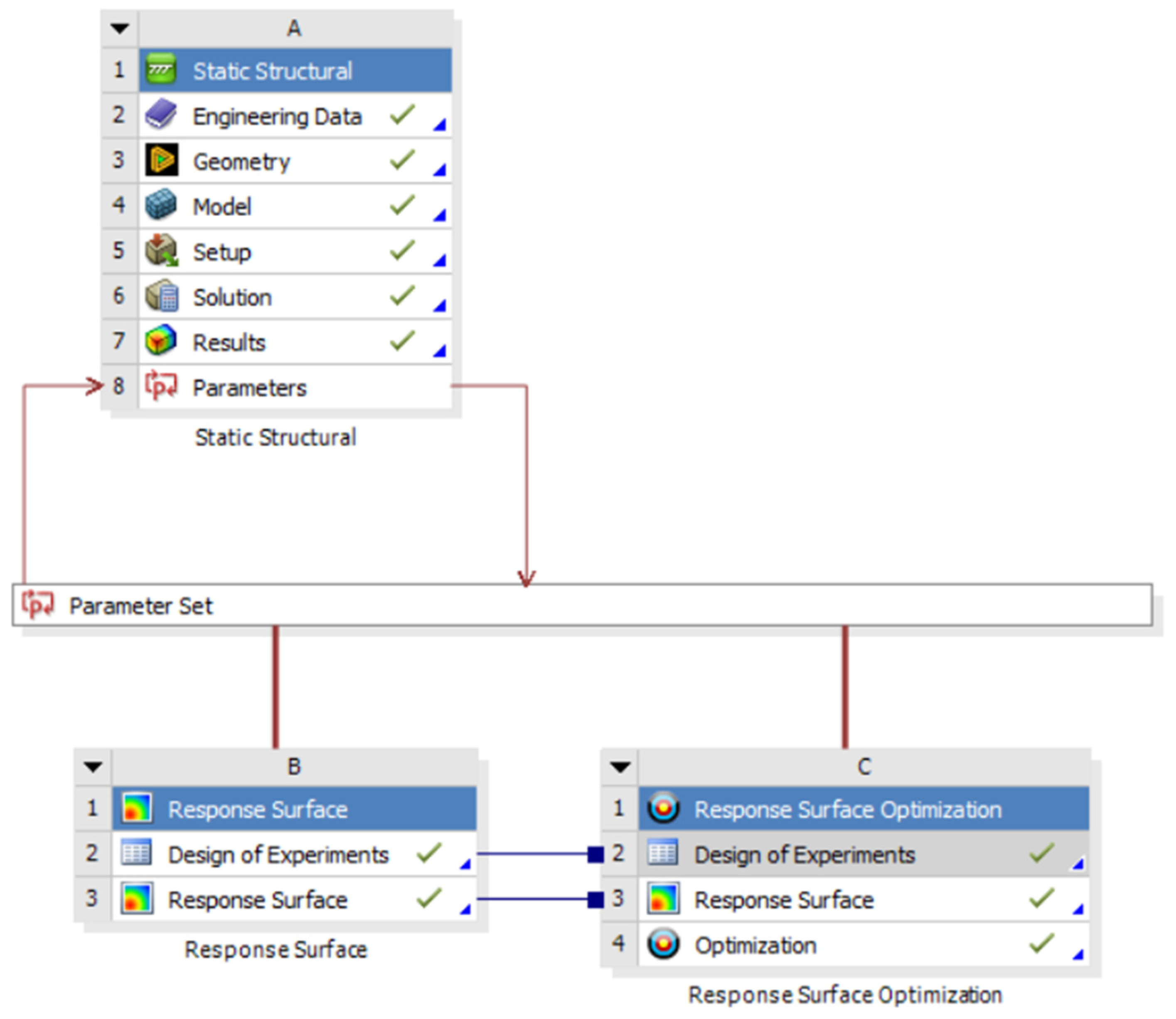
The structural optimization workflow (Figure 9) was implemented in ANSYS Workbench using a Static Structural system, where the material definition, parametric geometry, meshing, boundary conditions, and solution outputs were established in a single analysis chain. The identified geometric dimensions were exposed as input parameters in the Parameter Set, while the performance indicators (e.g., maximum deformation, maximum von Mises stress, and mass) were defined as output parameters. A Response Surface module was then employed to generate a surrogate model via a Design of Experiments (DoE), and the resulting response surfaces were subsequently used within the Response Surface Optimization environment to search for the optimal design under the imposed constraints.

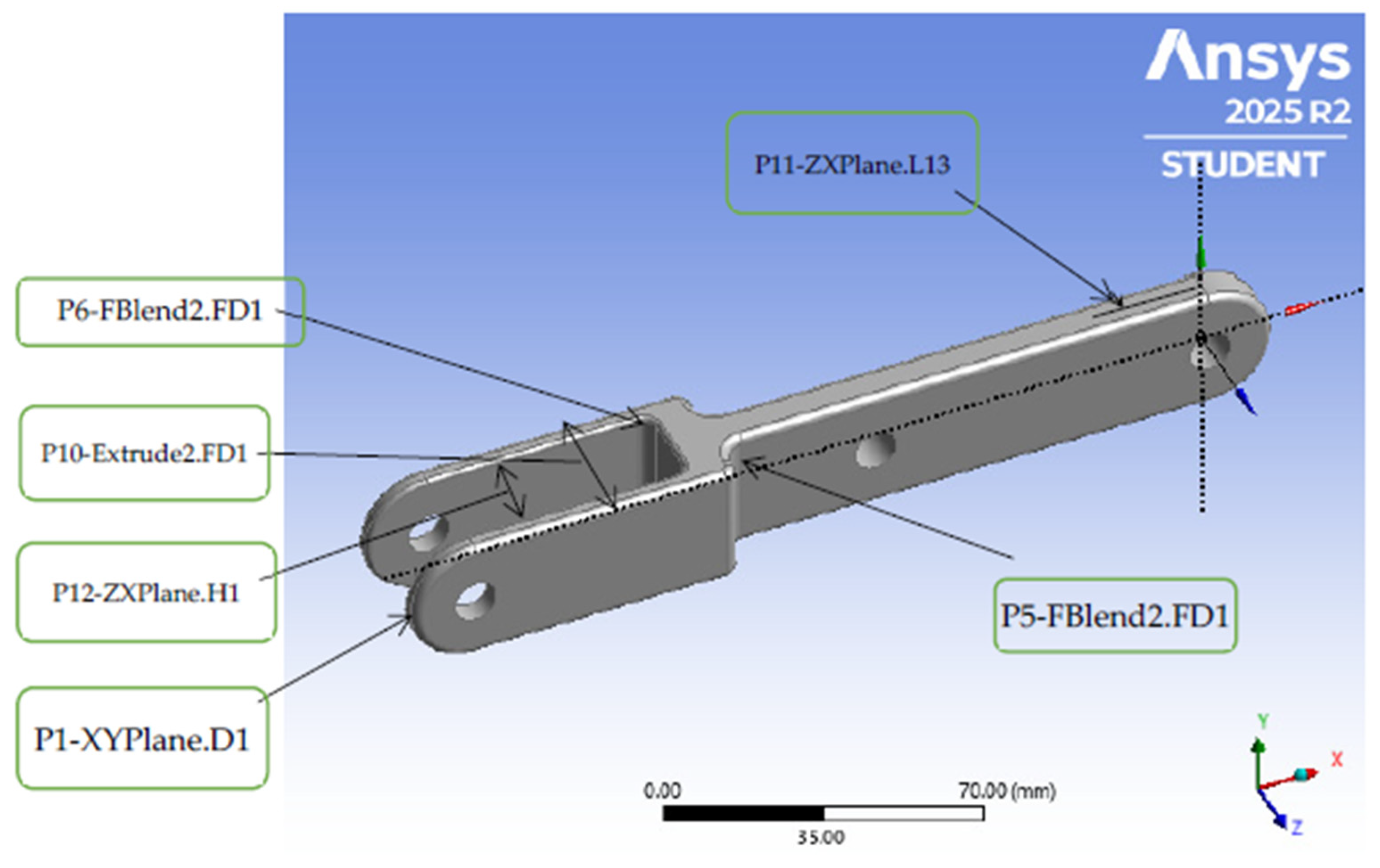
The CAD model was parameterized in ANSYS DesignModeler (Figure 10) and linked to the Workbench optimization environment through six geometric input parameters (

Table 2. Input parameters defined in ANSYS DesignModeler and exported to Workbench.

ID	Parameter Name (ANSYS)	Value (Units)	Description
P1	XYPlane.D1	30 mm	Outer circle diameter of the initial sketch; controls the link width (outer profile).
P5	FBlend1.FD1	5 mm	Primary fillet radius in the fork transition region.
P6	FBlend2.FD1	3 mm	Secondary fillet radius (parameterized blend).
P10	Extrude2.FD1	20 mm	Extrusion distance of the initial sketch; defines the part thickness in the fork region.
P11	ZXPlane.L13	5 mm	Symmetric extrusion distance with respect to the XY plane; defines the thickness of the fork-end region.
P12	ZXPlane.H1	20 mm	Gap between fork arms (slot width) generated by the Extrude Cut operation.

): P1-XYPlane.D1, P5-FBlend1.FD1, P6-FBlend2.FD1, P10-Extrude2.FD1, P11-ZXPlane.L13, and P12-ZXPlane.H1. The parameter P1-XYPlane.D1 controls the outer diameter of the initial sketch and therefore the link width. The blend radii FBlend1.FD1 and FBlend2.FD1 define the main and secondary fillets, respectively, governing stress concentration in the transition zones. The parameter Extrude2.FD1 represents the extrusion distance of the initial sketch and sets the thickness of the component in the fork region. The parameter ZXPlane.L13 defines the symmetric extrusion distance relative to the XY plane, controlling the thickness of the fork-end region (right-side end). Finally, ZXPlane.H1 specifies the gap between the fork arms, i.e., the slot width produced by the Extrude Cut operation.

4.2. Finite Element Model and Boundary Conditions

A parametric CAD model of the selected load-bearing link 2 (Figure 10) was imported into ANSYS Workbench and analyzed using Static Structural. The structural analyses in ANSYS Workbench were performed assuming an isotropic linear-elastic material model for PLA. The material properties introduced in Engineering Data were: Young’s modulus E = 3.2 GPa, Poisson’s ratio ν = 0.35, density ρ = 1240 kg/m³, and tensile strength σ = 70 MPa. These values were used consistently in the Static Structural simulations and in the stress-based design assessment adopted during optimization. It should be noted that the mechanical properties of FDM-printed PLA depend on printing orientation, infill density, and process parameters; therefore, the above values were adopted here as representative nominal properties for the present finite-element design study.

The component was discretized with 3D solid elements and a mesh refinement strategy focused on stress raisers (fillets and hole vicinities), where peak equivalent stress is expected. A local mesh control was applied along the parameterized blends (FBlend1.FD1 and FBlend2.FD1) and around the joint holes to ensure adequate stress resolution. Mesh quality and solution stability were verified by monitoring the variation in maximum equivalent stress and maximum total deformation under progressive refinement, adopting a mesh density that yielded negligible changes in these peak responses.

Boundary conditions were defined to reproduce the mechanical constraints induced by the adjacent links through revolute joints. The joint interfaces were modeled by constraining the corresponding cylindrical surfaces (or equivalent remote coupling at the joint center) such that rigid-body motion is prevented consistently with the physical assembly, while allowing the appropriate rotational degree of freedom associated with the joint. External loads were applied as resultant connection forces at the terminal joints, obtained from the mechanism operating conditions (i.e., joint force resultants during gait-assist motion). These forces generate the dominant internal stress state in the component and therefore provide a representative loading scenario for structural optimization. This modeling approach ensures that the optimization is driven by operational loads rather than arbitrary benchmark tests.

For the nominal geometry reported in the Workbench Parameter Set (Figure 10), the FE analysis returns the output responses P7 (Total Deformation Maximum), P8 (Equivalent Stress Maximum), and P9 (Solid Mass), which are subsequently used in the surrogate-based optimization workflow.

4.3. Design Variables, Constraints, and Output Metrics

The optimization variables were selected among geometric dimensions that directly influence stiffness, stress concentration, and mass, while remaining compatible with manufacturability and assembly clearances. Six input parameters were defined in ANSYS DesignModeler and exported to Workbench (Table 2 and Figure 10): XYPlane.D1 (P1), FBlend1.FD1 (P5), FBlend2.FD1 (P6), Extrude2.FD1 (P10), ZXPlane.L13 (P11), and ZXPlane.H1 (P12). During optimization, these inputs were allowed to vary within prescribed bounds selected to preserve functional requirements (e.g., joint-hole integrity, fork clearance, and minimum thickness) and manufacturability constraints.

The six geometric input parameters were allowed to vary within predefined bounds in Workbench: XYPlane.D1 (27–33 mm), FBlend1.FD1 (4.5–5.5 mm), FBlend2.FD1 (2.7–3.3 mm), Extrude2.FD1 (13.5–16.5 mm), ZXPlane.L13 (4.5–5.5 mm), and ZXPlane.H1 (18–22 mm). These ranges were selected to preserve assembly compatibility and manufacturability while enabling meaningful reductions in mass without compromising stiffness and strength.

The optimization was formulated using the following output metrics (parameters):

○

P7: Total Deformation Maximum—stiffness indicator (lower values imply higher rigidity);

○

P8: Equivalent Stress Maximum (von Mises)—strength/safety indicator;

○

P9: Solid Mass—weight indicator to be minimized.

Constraints were imposed to ensure mechanical feasibility under the representative operational loading. In particular, P8 was required to remain below an admissible equivalent stress (set according to the selected material and safety factor), while P7 was limited to maintain sufficient rigidity for gait-assist operation and joint alignment. The objective was to minimize P9 subject to these strength and stiffness constraints, effectively yielding lightweight but mechanically safe solutions.

The complete lists of the DoE design points, including the input parameter settings and the corresponding output responses (P7–P9), are provided in Appendix A.1 and Appendix A.2 (

Table A1. Design of Experiments (DoE) design points and input parameters defined in ANSYS Workbench.

Design Point (Name)	P1 XYPlane.D1 (mm)	P5 FBlend1.FD1 (mm)	P6 FBlend2.FD1 (mm)	P10 Extrude2.FD1 (mm)	P11 ZXPlane.L13 (mm)	P12 ZXPlane.H1 (mm)
1	30	5	3	15	5	20
2	27	5	3	15	5	20
3	33	5	3	15	5	20
4	30	4.5	3	15	5	20
5	30	5.5	3	15	5	20
6	30	5	2.7	15	5	20
7	30	5	3.3	15	5	20
8	30	5	3	13.5	5	20
9	30	5	3	16.5	5	20
10	30	5	3	15	4.5	20
11	30	5	3	15	5.5	20
12	30	5	3	15	5	18
13	30	5	3	15	5	22
14	28.3	4.7	2.8	14.1	4.7	18.8
15	31.7	4.7	2.8	14.1	4.7	21.2
16	28.3	5.3	2.8	14.1	4.7	21.2
17	31.7	5.3	2.8	14.1	4.7	18.8
18	28.3	4.7	3.2	14.1	4.7	21.2
19	31.7	4.7	3.2	14.1	4.7	18.8
20	28.3	5.3	3.2	14.1	4.7	18.8
21	31.7	5.3	3.2	14.1	4.7	21.2
22	28.3	4.7	2.8	15.9	4.7	21.2
23	31.7	4.7	2.8	15.9	4.7	18.8
24	28.3	5.3	2.8	15.9	4.7	18.8
25	31.7	5.3	2.8	15.9	4.7	21.2
26	28.3	4.7	3.2	15.9	4.7	18.8
27	31.7	4.7	3.2	15.9	4.7	21.2
28	28.3	5.3	3.2	15.9	4.7	21.2
29	31.7	5.3	3.2	15.9	4.7	18.8
30	28.3	4.7	2.8	14.1	5.3	21.2
31	31.7	4.7	2.8	14.1	5.3	18.8
32	28.3	5.3	2.8	14.1	5.3	18.8
33	31.7	5.3	2.8	14.1	5.3	21.2
34	28.3	4.7	3.2	14.1	5.3	18.8
35	31.7	4.7	3.2	14.1	5.3	21.2
36	28.3	5.3	3.2	14.1	5.3	21.2
37	31.7	5.3	3.2	14.1	5.3	18.8
38	28.3	4.7	2.8	15.9	5.3	18.8
39	31.7	4.7	2.8	15.9	5.3	21.2
40	28.3	5.3	2.8	15.9	5.3	21.2
41	31.7	5.3	2.8	15.9	5.3	18.8
42	28.3	4.7	3.2	15.9	5.3	21.2
43	31.7	4.7	3.2	15.9	5.3	18.8
44	28.3	5.3	3.2	15.9	5.3	18.8
45	31.7	5.3	3.2	15.9	5.3	21.2

and

Table A2. Design of Experiments (DoE) design points and output responses obtained from Static Structural analysis.

Design Point (Name)	P7—Total Deformation Maximum (mm)	P8—Equivalent Stress Maximum (MPa)	P9—Solid Mass (kg)
1	0.187786	54.100817	0.503684
2	0.243600	59.607657	0.445931
3	0.150648	51.084358	0.562546
4	0.188436	54.260311	0.503198
5	0.187144	53.681666	0.504220
6	0.187973	53.630122	0.503510
7	0.187590	53.559845	0.503875
8	0.239031	76.966137	0.452741
9	0.160834	41.274162	0.554626
10	0.195124	53.921280	0.474575
11	0.181649	54.265308	0.532792
12	0.165741	44.571841	0.532969
13	0.220447	67.840272	0.474398
14	0.229051	59.689822	0.442389
15	0.212987	73.505499	0.469575
16	0.279542	79.714028	0.411479
17	0.172833	55.564324	0.506486
18	0.280160	79.615100	0.411121
19	0.173291	55.740792	0.506085
20	0.227925	60.103875	0.443145
21	0.212006	73.146621	0.470423
22	0.216963	53.219080	0.465759
23	0.144005	40.750654	0.568872
24	0.189823	44.743881	0.497783
25	0.163645	49.066064	0.533210
26	0.190373	44.720798	0.497425
27	0.164158	49.295557	0.532809
28	0.215730	53.255017	0.466516
29	0.143194	40.694851	0.569720
30	0.271218	79.567626	0.442371
31	0.166870	55.560546	0.541734
32	0.219180	60.184589	0.474395
33	0.205524	73.211547	0.506073
34	0.219679	59.720504	0.474037
35	0.205987	73.824996	0.505671
36	0.269999	79.761397	0.443127
37	0.166098	55.640436	0.542583
38	0.181593	43.950074	0.528676
39	0.157651	49.467944	0.568459
40	0.206883	56.609619	0.497766
41	0.136846	40.653254	0.605370
42	0.207442	52.942113	0.497408
43	0.137249	40.295906	0.604969
44	0.180602	43.871197	0.529432
45	0.156779	49.016450	0.569307

).

4.4. Response Surfaces and Multi-Objective Genetic Optimization (MOGA)

To efficiently explore the multi-parameter design space without performing an excessive number of full FE evaluations, the optimization was conducted using DesignXplorer within ANSYS Workbench (Figure 9). First, a Design of Experiments (DoE) plan was generated over the bounds of the six input parameters (P1, P5, P6, P10, P11, P12) to sample the response behavior across the feasible region. Each DoE design point was evaluated through the Static Structural analysis, and the resulting outputs P7–P9 were collected.

Based on the DoE database, response surface surrogate models were constructed to approximate the mapping between the geometric inputs and the response metrics (deformation, stress, and mass). Surrogate accuracy was checked through internal validation indicators (e.g., goodness-of-fit and prediction error statistics provided by Workbench), ensuring that the approximations remain reliable in the sampled domain.

Subsequently, the multi-criteria search was performed using the Multi-Objective Genetic Algorithm (MOGA) on the surrogate models, enabling an efficient identification of trade-off solutions. The algorithm targets a balanced exploration of competing objectives—primarily reducing P9 while simultaneously satisfying constraints on P7 and P8—and produces a set of non-dominated candidate designs (Pareto-optimal solutions) that quantify the mass–stiffness–strength trade-off.

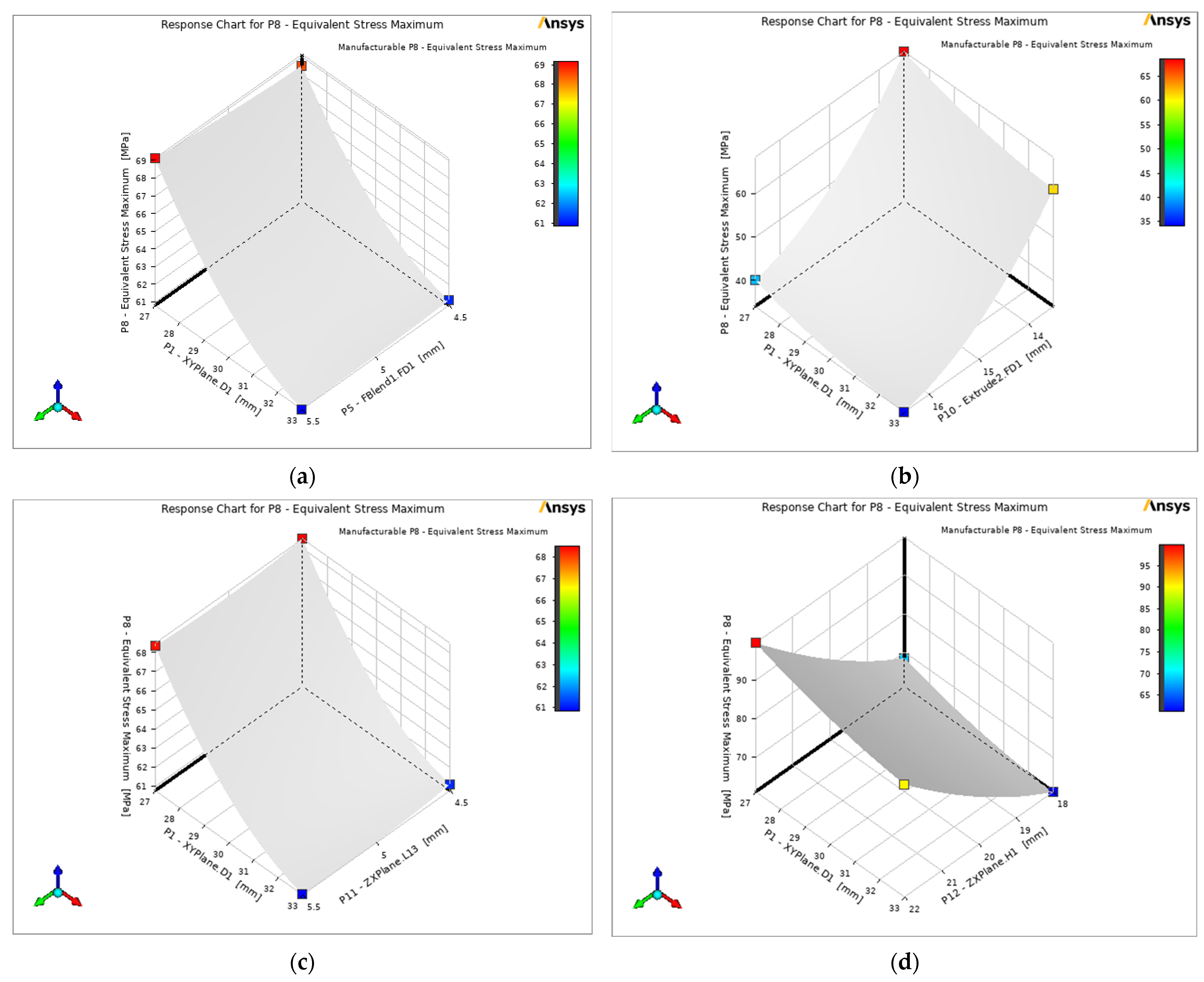
Response surface charts were generated in ANSYS DesignXplorer to visualize the influence of the most relevant geometric input parameters on the maximum equivalent (von Mises) stress P8 (Figure 11), thereby supporting the subsequent MOGA-based search for feasible lightweight designs.

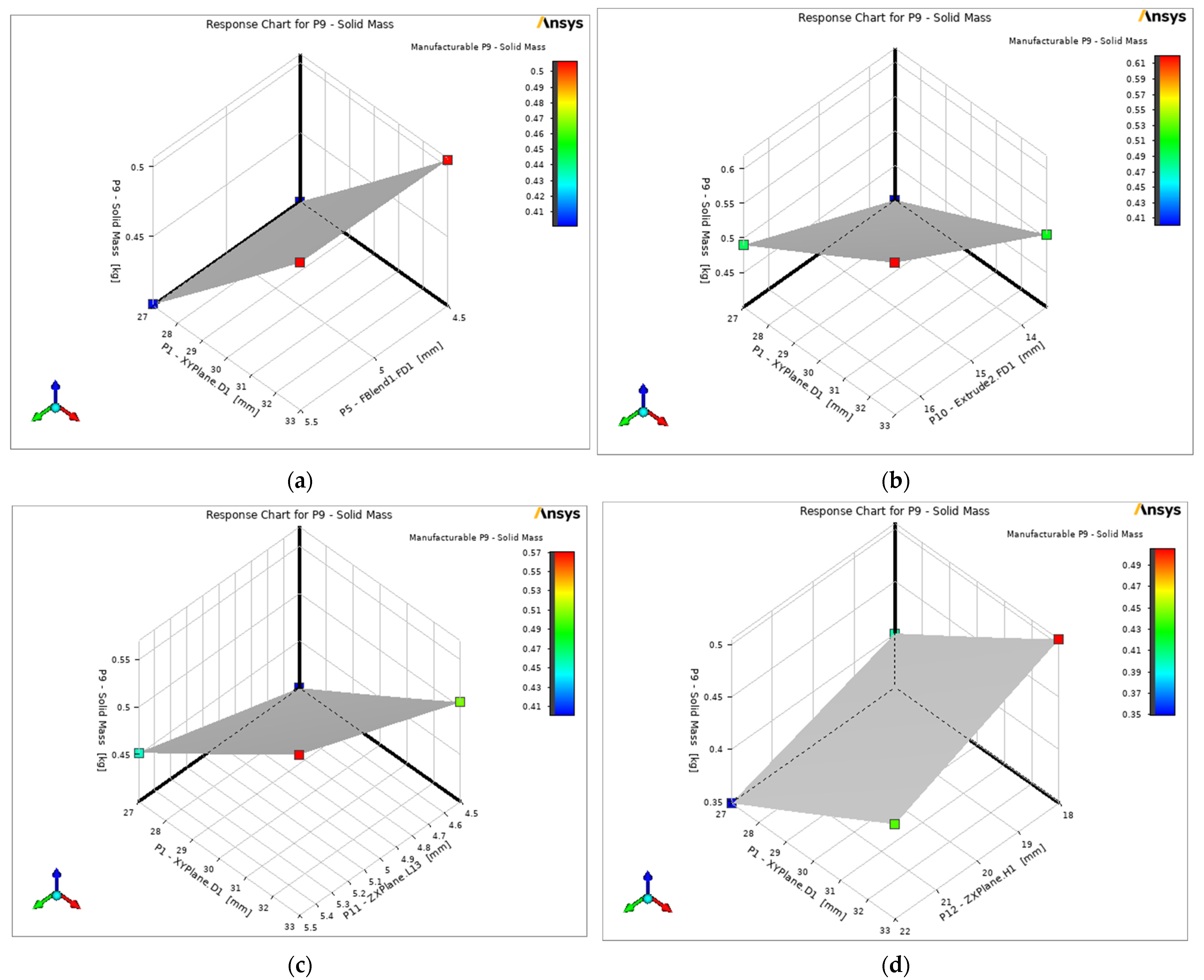
Additional response surface charts were built for the mass response P9 (Figure 12) to quantify how the key geometric input parameters affect the component weight and to support the selection of lightweight designs under the imposed stress and deformation constraints.

Overall, these response surfaces confirm a clear mass–stiffness–strength coupling, highlighting the most influential geometric parameters and providing a reliable basis for the subsequent MOGA search toward minimum-mass solutions that satisfy the stress and deformation limits.

4.5. Selection of the Optimal Design and Extension to the Full Mechanism

Based on the response surfaces and the MOGA-driven search, the final configuration was selected from the feasible candidates by enforcing strict compliance with the imposed constraints on deformation and stress, namely P7 ≤ 0.2 mm and P8 ≤ 50 MPa, while targeting P7 → 0 mm and P8 → 0 MPa as guiding objectives and minimizing the component mass P9. The optimization converged after 64 evaluations, yielding a small set of candidate solutions (

Table 3. Optimization objectives, constraints, and candidate solutions obtained by MOGA in ANSYS Workbench.

Item	Candidate Point 1	Candidate Point 2	Candidate Point 3
Optimization Study
Seek P7 = 0 mm; P7 ≤ 0.2 mm	Goal: seek P7 = 0 mm (default importance); strict constraint: P7 values ≤ 0.2 mm (default importance).
Seek P8 = 0 MPa; P8 ≤ 50 MPa	Goal: seek P8 = 0 MPa (default importance); strict constraint: P8 values ≤ 50 MPa (default importance).
Minimize P9	Goal: minimize P9 (default importance).
Optimization Method
MOGA	The MOGA method (Multi-Objective Genetic Algorithm) is a variant of NSGA-II. It supports multiple objectives and constraints and aims at finding the global optimum.
Configuration	Generate 100 samples initially, 100 samples per iteration and find 3 candidates in a maximum of 20 iterations.
Status	Converged after 64 evaluations, because all permutations have been evaluated.
Candidate Points
Parameter	Candidate Point 1	Candidate Point 2	Candidate Point 3
P1—XYPlane.D1 (mm)	27	27	33
P5—FBlend1.FD1 (mm)	4.5	5.5	4.5
P6—FBlend2.FD1 (mm)	3.3	3.3	2.7
P10—Extrude2.FD1 (mm)	16.5	16.5	16.5
P11—ZXPlane.L13 (mm)	5.5	5.5	4.5
P12—ZXPlane.H1 (mm)	18	18	22
P7—Total Deformation Maximum (mm)	0.18752	0.1862	0.1598
P8—Equivalent Stress Maximum (MPa)	39.147	40.016	49.678
P9—Solid Mass (kg)	0.54211	0.54303	0.55357

) that satisfy the stiffness–strength requirements and exhibit reduced mass.

Among the reported candidates, Candidate Point 1 provides the best trade-off in terms of minimum mass under constraints, with the following parameter values: P1 = 27 mm, P5 = 4.5 mm, P6 = 3.3 mm, P10 = 16.5 mm, P11 = 5.5 mm, and P12 = 18 mm. The corresponding responses are P7 = 0.1875 mm, P8 = 39.15 MPa, and P9 = 0.5421 kg, confirming that the solution remains safely below the admissible stress limit and within the deformation requirement, while achieving the lowest mass among the feasible candidates. Candidate Points 2 and 3 also satisfy the constraints; however, they lead to slightly higher mass values (P9 = 0.5430 kg and P9 = 0.5536 kg, respectively) or to less favorable combinations of stiffness and weight compared to Candidate Point 1.

The selected optimal geometry was subsequently validated by a full Static Structural re-analysis using the exact CAD parameter values in Workbench, confirming the predicted outputs (P7–P9) under the same operational boundary conditions. The optimized component was then exported for rapid prototyping and assembly integration into the leg exoskeleton mechanism.

Finally, the same parameterization–DoE–response surface–MOGA workflow can be systematically applied to the remaining load-bearing links of the exoskeleton leg. By using representative joint loading for each component, the overall structural mass can be reduced at the mechanism level while preserving adequate stiffness and strength, thereby improving portability and reducing actuator requirements.

A corresponding virtual prototype of this configuration was developed following the modeling workflow previously reported in [36] (Figure 13), enabling subsequent kinematic and dynamic investigations in MSC ADAMS. In Figure 13, the different colors are used only for visual differentiation of the exoskeleton components, making it easier to identify the corresponding links, supporting frame elements, and moving leg members in the ADAMS virtual prototype.

5. Multibody Dynamic Simulations for Motion Assessment and Load Extraction in MSC ADAMS

In the ADAMS environment, the exoskeleton leg was modeled as a planar multibody system composed of rigid links connected through revolute joints, consistent with the synthesized mechanism topology. The hip and knee joints are represented by the revolute pairs between the femur-like link and the base (hip) and between femur- and tibia-like links (knee), while the ankle point M is used as the main tracking point to evaluate gait-related motion characteristics (trajectory, velocity, and displacement components).

5.1. Model Setup, Actuation, and Simulation Outputs

The multibody model was assembled by defining: (i) the rigid bodies and their inertial properties, (ii) the kinematic joints reproducing the mechanism connectivity, and (iii) an actuation input applied to the driving link of the Chebyshev–pantograph powertrain. The input motion was prescribed through a rotational driver (angle/time law) or an equivalent torque input, depending on the simulation objective (pure kinematics vs. dynamic response).

Ground contact was defined in MSC ADAMS as a solid-to-solid interaction using the IMPACT normal-force model and Coulomb friction. The adopted model unit system was MMKS (mm, kg, N, s). The normal contact parameters were stiffness K = 1000.0, force exponent e = 2.0, damping C = 400.0, and penetration depth d = 1.5. The tangential contact model used static and dynamic friction coefficients of 0.35 and 0.30, respectively, with both stiction and friction transition velocities set to 10.0. The same contact parameter set was used for the level-ground, ramp, and stair simulations.

The following output quantities were computed to characterize the mechanism performance and to generate load cases for structural assessment:

○

angular histories in the hip and knee joints;

○

trajectory and displacement components of point M (used as an ankle surrogate);

○

joint reaction forces in the main revolute pairs (particularly in hip and knee joints);

○

required drive torque and selected kinematic indicators (velocity/acceleration of the end-point).

5.2. Simulation Scenarios in ADAMS

To assess the exoskeleton behavior in representative assistance conditions, several simulation scenarios were considered:

✓

Fixed-frame evaluation: the upper frame is constrained relative to the ground, to isolate the mechanism motion and verify the gait-like trajectory of point M (useful for comparing structural solutions under identical actuation).

✓

Level-ground progression: the model is simulated under forward progression conditions, enabling evaluation of point M motion (ankle), joint angles, and joint reactions during a representative gait cycle.

✓

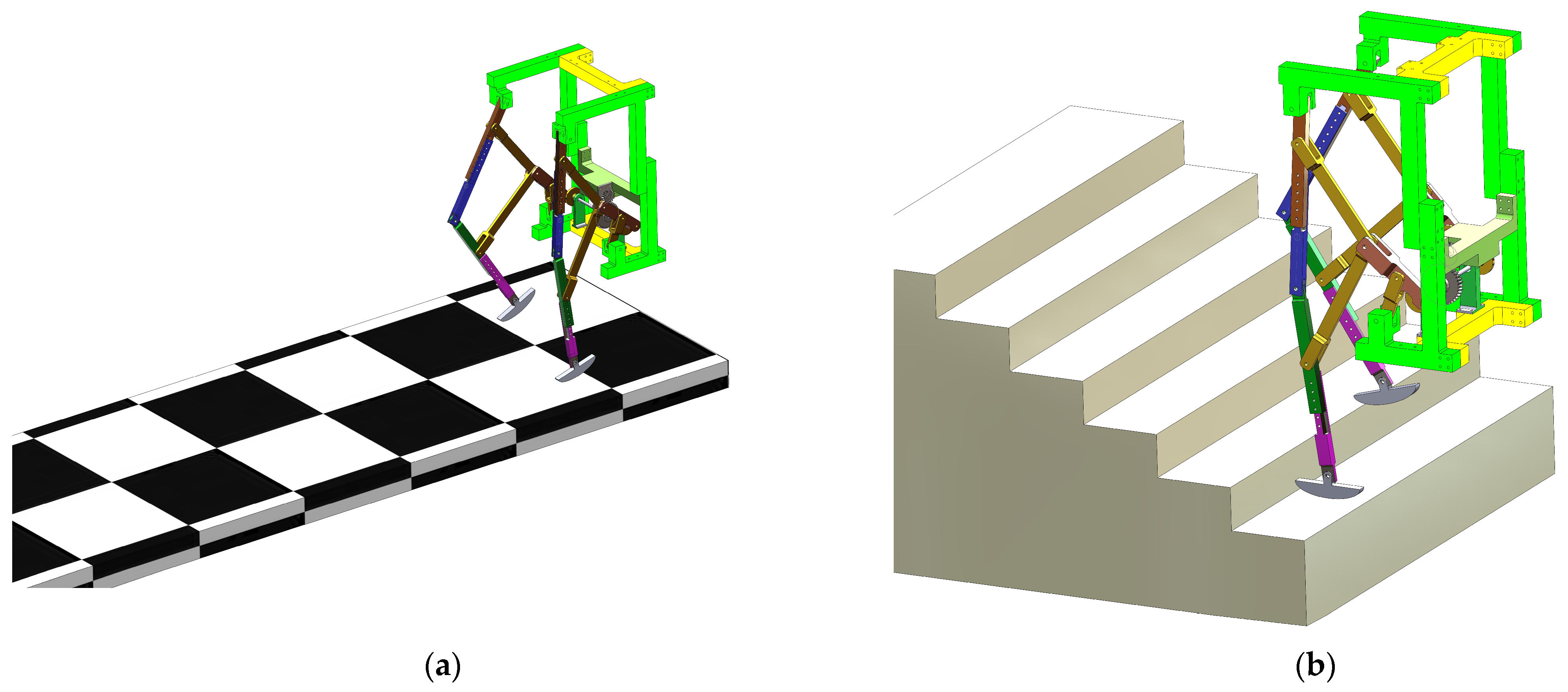
Stair-climbing assistance: the environment is represented by step geometry and the motion is simulated to reproduce the required foot clearance and elevation profile.

✓

Ramp ascent: an inclined plane is introduced to evaluate changes in kinematics and joint loading under slope conditions.

These scenarios provide both performance indicators (workspace suitability, smoothness, and feasible joint excursions) and—most importantly for Section 4—representative joint load histories that can be transferred to the finite element model.

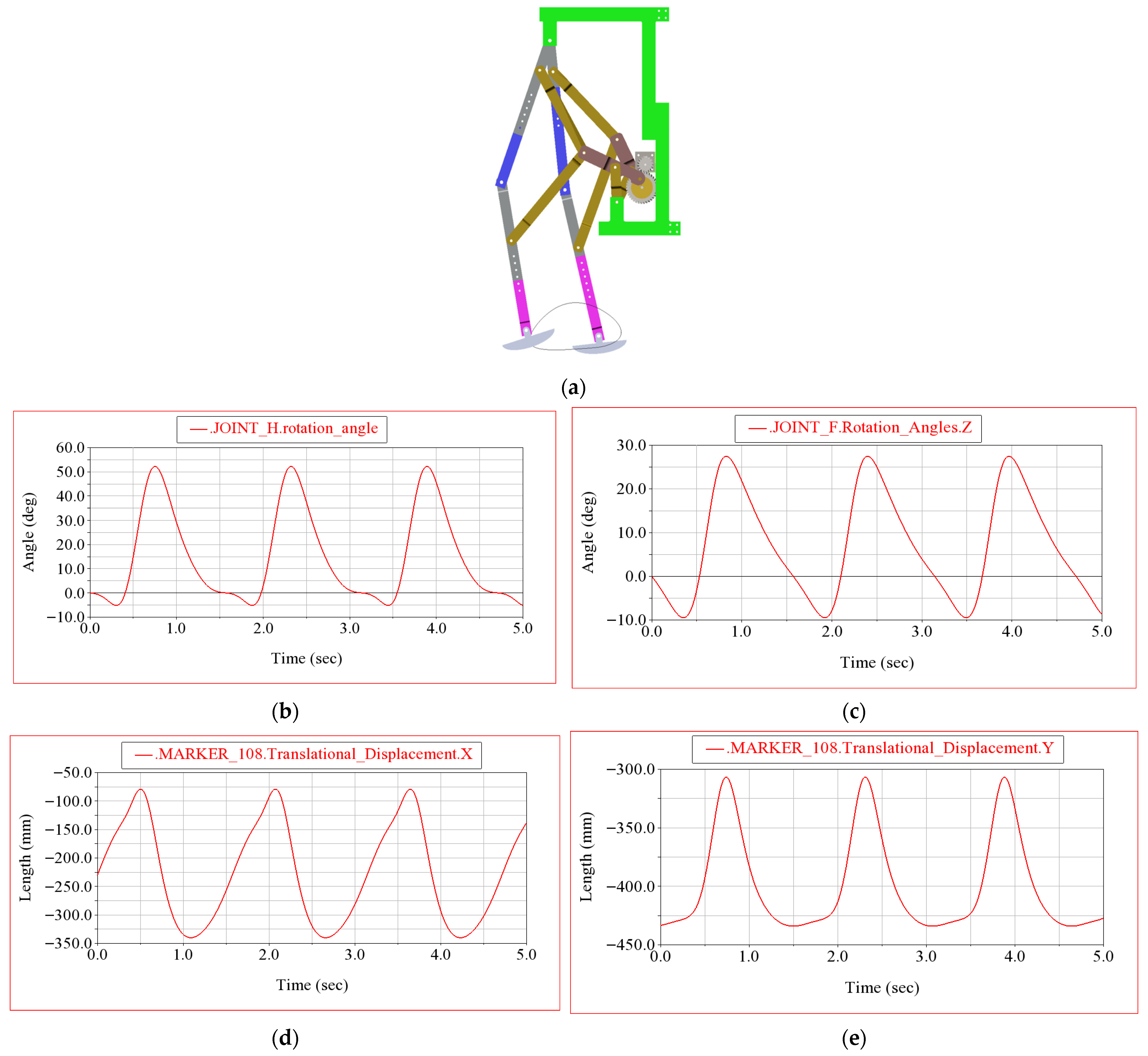
In the fixed-frame scenario (Figure 14), the mechanism generates a repeatable ovoid foot-point trajectory, evidenced by the periodic X–Y motion of MARKER_108 (point M) over three consecutive cycles (0–5 s). The horizontal displacement varies approximately between −335 mm and −85 mm (stroke ΔX ≈ 250 mm), while the vertical displacement varies approximately between −440 mm and −310 mm (lift ΔY ≈ 130 mm). The waveform in Y shows a pronounced peak during each cycle, corresponding to the swing/clearance phase, whereas the lower, flatter portion corresponds to the stance-like phase. From the repeated peaks, the motion period is about 1.7 s (≈0.6 Hz), confirming stable and consistent cycle-to-cycle behavior.

The joint rotation histories further support the gait-like pattern. The knee joint (JOINT_H) exhibits a larger excursion, ranging roughly from ≈−2° to ≈48°, with a sharp flexion peak followed by extension within each cycle. The hip joint (JOINT_F) shows a smaller but synchronized motion, ranging approximately from ≈−7° to ≈27°. Notably, the knee flexion peaks occur close to the intervals where the vertical displacement Y reaches its maximum, which is consistent with the expected coordination between hip–knee motion and foot clearance. Overall, the fixed-frame results confirm that the Chebyshev–pantograph architecture can reproduce a repeatable, gait-relevant end-point motion while maintaining smooth, bounded joint rotations suitable for subsequent load extraction and dynamic cases with contact.

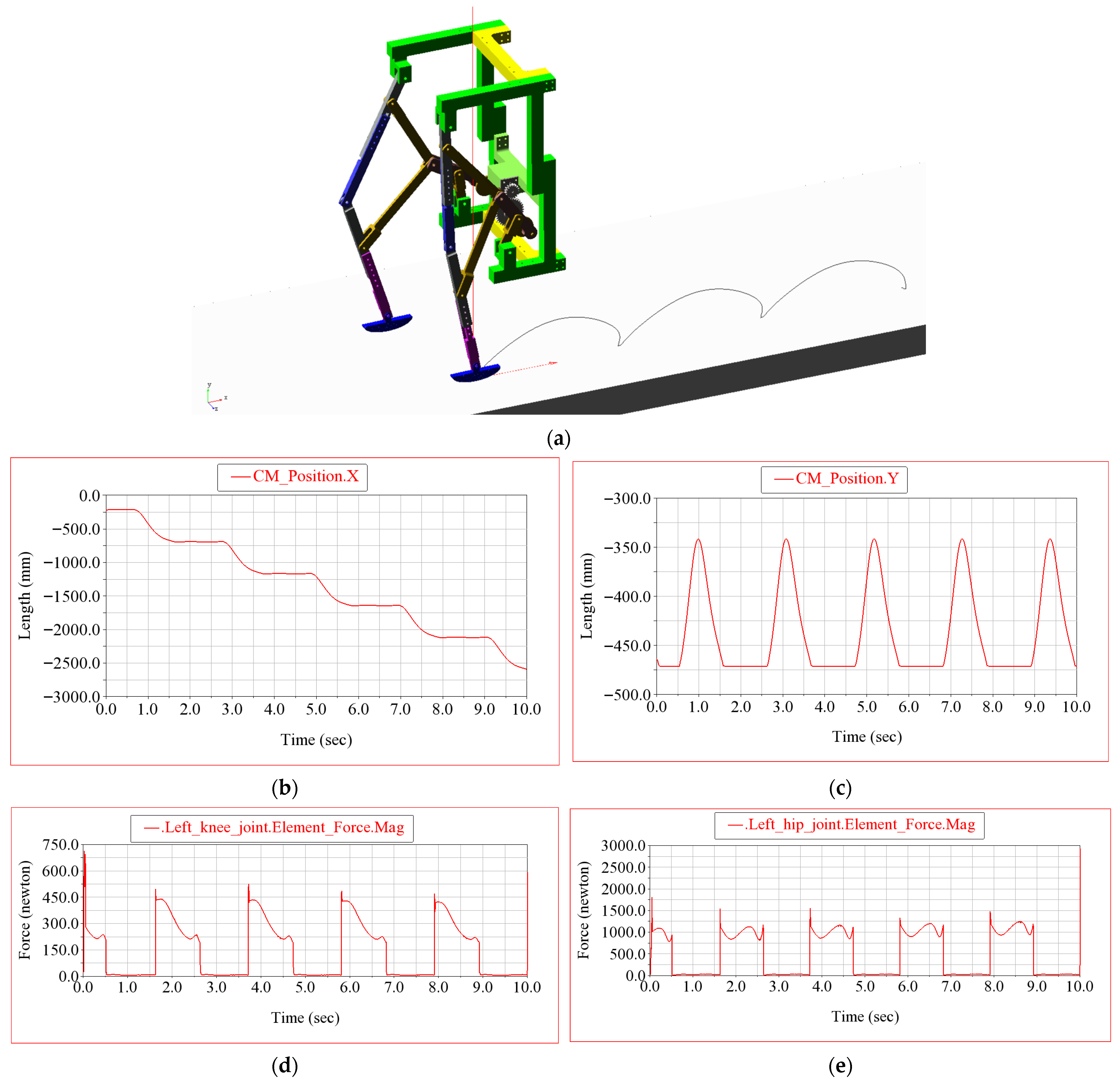
In Scenario 2, the exoskeleton performs forward progression on a horizontal plane (Figure 15a, see also Video S1 in the Supplementary Material). The CM horizontal position (Figure 15b) decreases monotonically in a step-like manner, indicating successive gait cycles with alternating support and swing phases. Over the simulated interval from 0 to 10 s, the CM advances from approximately −0.52 m to −2.60 m, i.e., a net progression of about 2.08 m, corresponding to an average forward speed of roughly 0.21 m/s (sign depends on the global axis orientation). The curve shows about five repeated “steps” over 10 s, giving a cycle period close to 2.0 s. The CM vertical position (Figure 15c) remains periodic and stable, oscillating between about −465 mm and −345 mm (vertical excursion ΔY ≈ 120 mm). The repeated peaks in Y correspond to the leg lift/clearance phase, while the lower plateau-like regions correspond to stance-like intervals. The different colors adopted in the ADAMS model serve only to visually differentiate the main structural and kinematic components of the exoskeleton, thus improving the clarity of the virtual prototype representation.

The dynamic load transfer during horizontal plane progression is reflected by the joint element forces. The left knee joint force magnitude (Figure 15d) exhibits clear cyclic peaks of approximately 0.39–0.40 kN at each step, followed by a decay during the remainder of the cycle, consistent with peak loading during support and push-off. The left hip joint force magnitude (Figure 15e) remains higher overall, reaching peaks of about 1.3–1.4 kN, with a repeated modulation synchronized with the gait cycle. Importantly, the force histories are repeatable across cycles, confirming numerical stability and providing a consistent basis for extracting representative joint loads to be transferred as boundary conditions for the subsequent structural evaluation and optimization stages.

Accordingly, the peak resultant reaction forces at the left knee and left hip joints obtained from Figure 15d,e were exported from ADAMS and subsequently applied as representative loading conditions in the ANSYS Static Structural model for the load-bearing links.

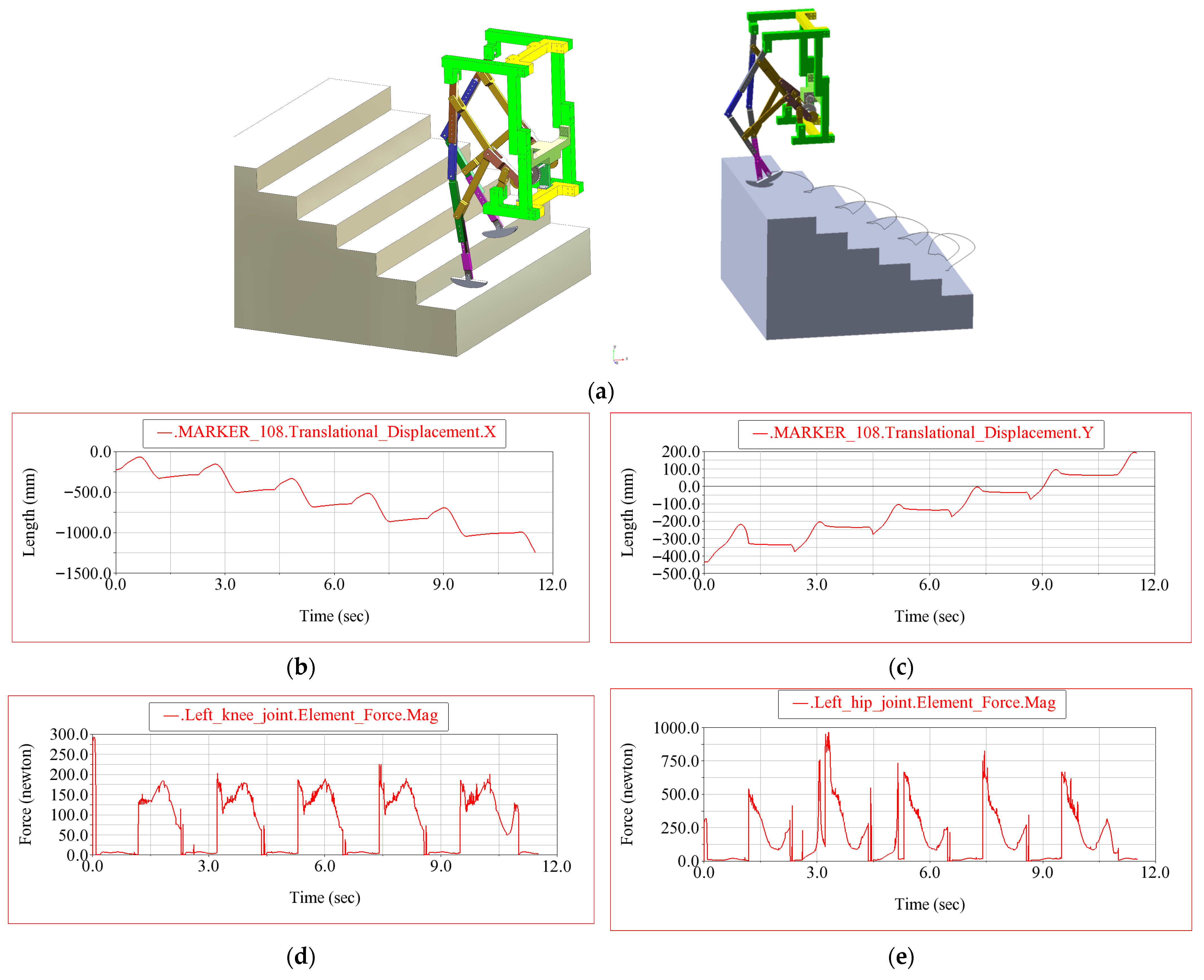
In Scenario 3, the exoskeleton performs stair ascent, which produces a distinct step-wise evolution of the end-point motion (Figure 16a–c). The horizontal displacement of point M (MARKER_108) (Figure 16b) decreases in a staircase-like pattern from approximately −0.1 m to −1.2 m over 0–12 s, corresponding to a net progression of about 1.1 m. In parallel, the vertical displacement (Figure 16c) increases progressively, from roughly −0.35 m up to about +0.15–0.20 m, i.e., a total elevation gain of approximately 0.50–0.55 m. The repeated plateaus and jumps in both X and Y are consistent with successive step negotiations, where swing phases produce rapid transitions and stance phases produce quasi-stationary intervals.

The stair-climbing task leads to more pronounced load variations in the joints (Figure 16d,e). The left knee joint element force magnitude reaches cyclic peaks on the order of 200–250 N, with repeated bursts associated with step contact and push-off. The left hip joint element force magnitude exhibits larger and sharper peaks, approaching approximately 0.9–1.0 kN, reflecting the increased demand during vertical lifting and support transfer on the stairs. As in the previous scenarios, the peak resultant reaction forces at the knee and hip joints were exported from ADAMS and used as representative loading conditions in the ANSYS Static Structural analyses of the load-bearing links.

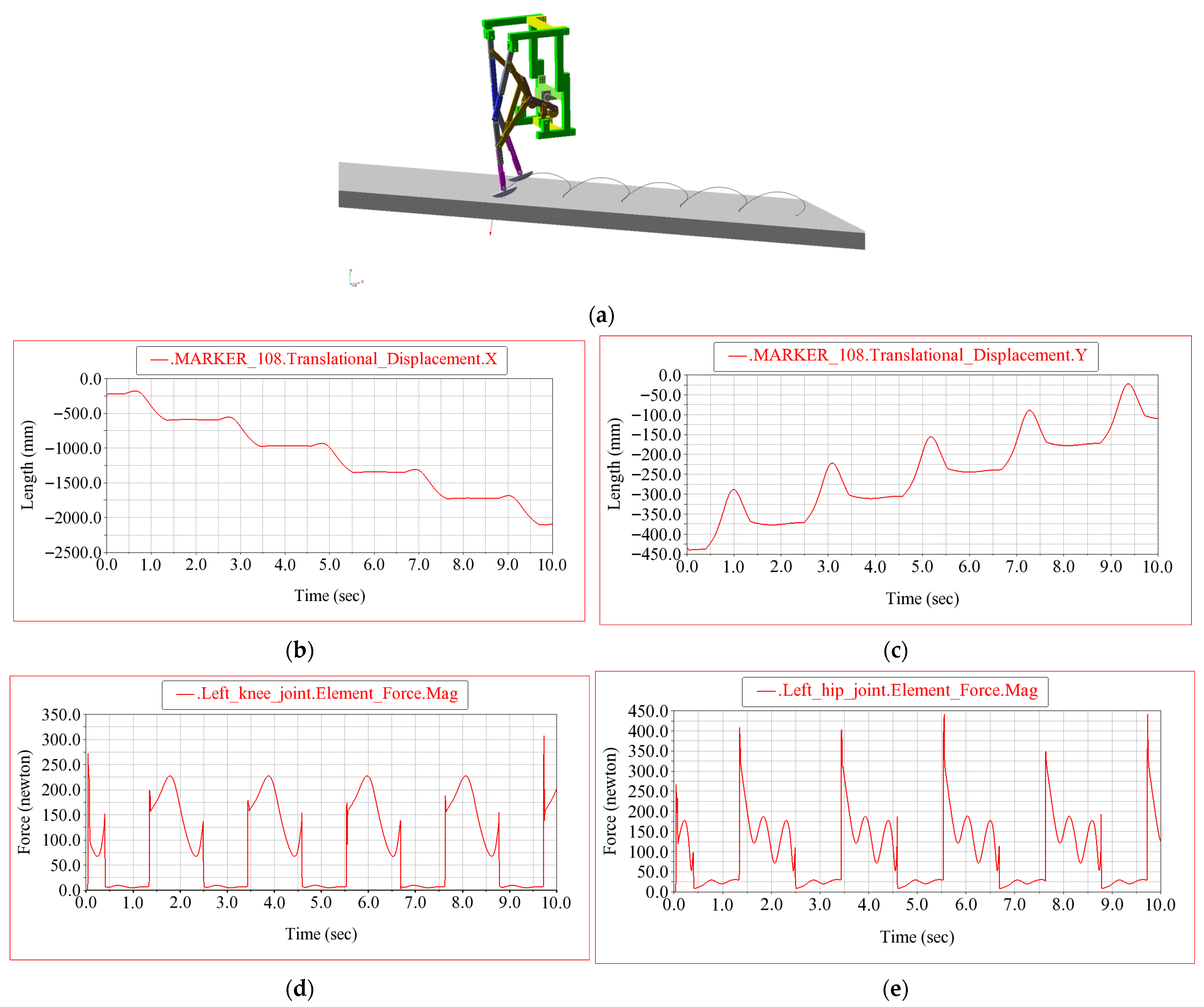
In the inclined-plane walking scenario (Figure 17a), the end-point M (MARKER_108) exhibits a clear step-wise progression. The horizontal displacement X (Figure 17b) decreases from approximately 0 mm to about −2300 mm over 0–10 s, resulting in a net progression of roughly 2.3 m (axis sign depends on the global reference frame). This corresponds to an average forward speed of about 0.23 m/s. The staircase-like profile indicates successive gait cycles, with nearly periodic drops in X associated with repeated stance-to-swing transitions.

The vertical displacement Y (Figure 17c) shows a progressive rise while maintaining a cyclic pattern, consistent with ascending a slope. Over the same interval, Y increases from approximately −430 mm up to about −60…−50 mm, i.e., a total elevation gain of roughly 0.37–0.38 m in the chosen global coordinate system (the absolute offset is coordinate-dependent; the trend and increments are physically meaningful). The repeated “bumps” in Y correspond to successive clearance events during swing, superimposed on the overall upward trend imposed by the inclined plane.

The dynamic loading is reflected in the joint force histories (Figure 17d,e). The left knee joint element force magnitude (Figure 17d) presents repeatable peaks typically around 200–260 N, with occasional higher spikes approaching ~300 N near cycle transitions. The left hip joint element force magnitude (Figure 17e) is higher overall, with frequent peaks in the range of ~250–400 N and sporadic spikes up to approximately ~450 N, indicating increased demand during support transfer and uphill propulsion. The peak resultant reaction forces at the knee and hip joints were exported from ADAMS and subsequently applied as representative loading conditions in the ANSYS Static Structural model for the load-bearing links.

Compared to the staircase case (Figure 16), the inclined-plane walking scenario yields a more regular progression pattern, with generally lower and less impulsive joint-force peaks, while still confirming that the hip joint remains the dominant load path during uphill propulsion.

5.3. Exoskeleton–Virtual Mannequin Coupled Simulation in MSC ADAMS

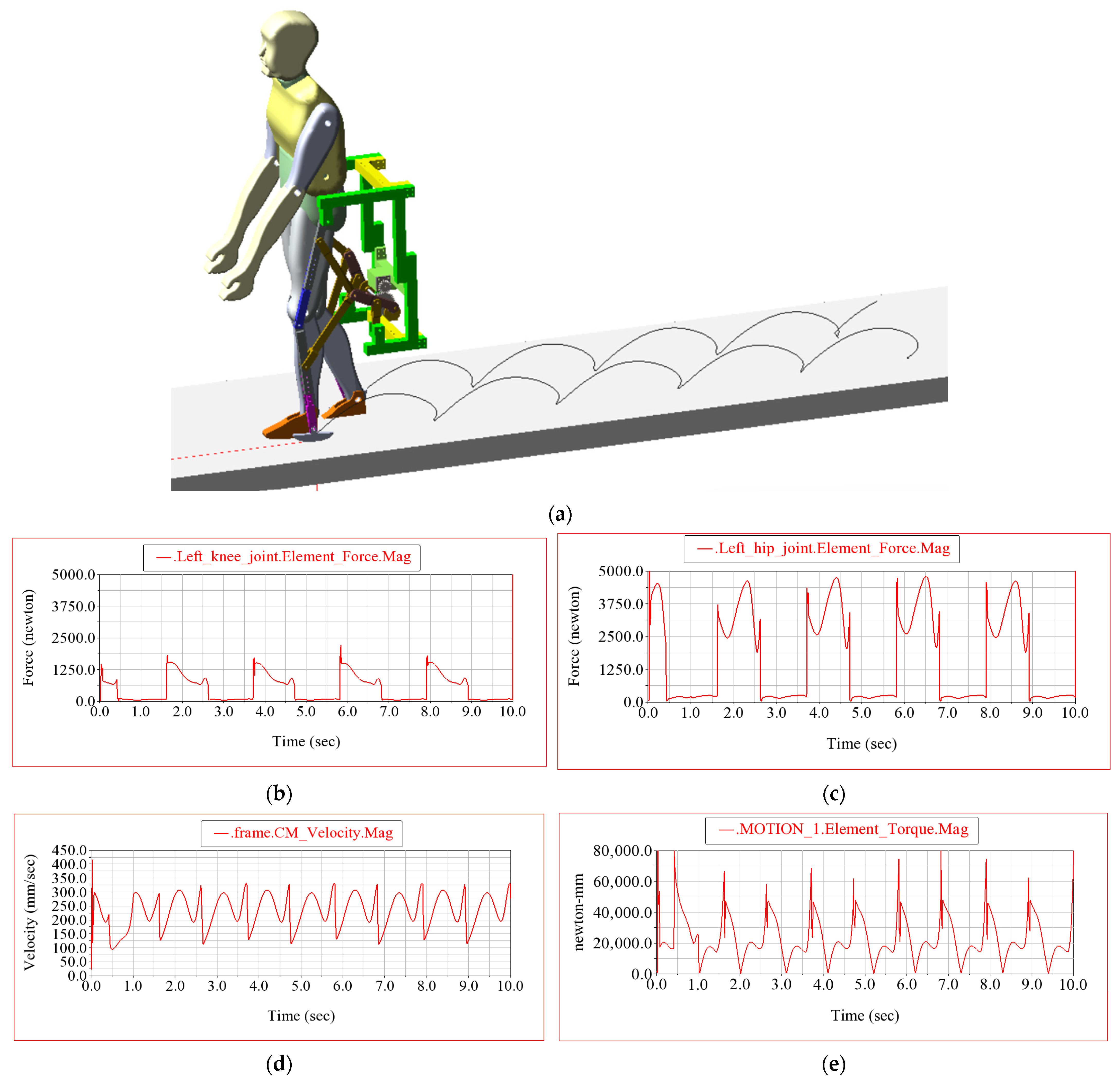
To obtain gait-relevant joint loads representative of human-assisted gait, the exoskeleton multibody model was coupled with a virtual mannequin in MSC ADAMS (Figure 15a). The mannequin provides a biomechanically meaningful reference for segment proportions, joint locations, and inertial properties, while the coupling was implemented by aligning the exoskeleton hip and knee revolute joints with the corresponding mannequin joint centers and by defining kinematic constraints between the exoskeleton attachment points and the corresponding thigh and shank segments. In this configuration, the exoskeleton guides the sagittal-plane motion, whereas the mannequin contributes realistic limb geometry and inertia. Compared with a stand-alone mechanism simulation, this mannequin-coupled setup yields more representative joint reactions because it captures the inertia-driven load transfer during support and swing phases under forward progression.

The virtual mannequin used in the coupled MSC ADAMS simulations represents a nominal adult subject with a total body mass of 70 kg and body height of 1.68 m. Based on standard anthropometric proportions and body-segment parameter tables, the lower-limb dimensions used in the present model were estimated as follows: thigh length 411.6 mm, shank length 413.3 mm, and effective foot segment length 255.4 mm. The corresponding segment masses were 7.00 kg for the thigh, 3.255 kg for the shank, and 1.015 kg for the foot. For the sagittal-plane multibody model, the representative centroidal mass moments of inertia about the mediolateral axes were taken as 0.124 kg·m² for the thigh, 0.051 kg·m² for the shank, and 0.015 kg·m² for the foot. These values were adopted as nominal literature-based estimates for the mannequin-coupled simulations [36,37].

The coupled model enables direct extraction of reaction forces and moments in the exoskeleton joints under gait-like motion, which are subsequently used as input loads for the structural analyses in ANSYS (Section 4). Compared to a stand-alone mechanism simulation, the mannequin-coupled approach improves the physical relevance of the computed joint reactions because it accounts for the inertia of the limb segments and preserves realistic joint kinematics and segment coordination. Consequently, the resultant connection forces obtained in the terminal joints during operation are treated as representative operational loads for the optimization-driven design of the load-bearing links.

In the present work, biomechanical compatibility is addressed at a nominal first-order level by aligning the exoskeleton hip and knee revolute joints with the corresponding mannequin joint centers in the reference posture, by adapting the main leg dimensions to the intended user geometry, and by restricting assistance to sagittal-plane flexion/extension. However, no explicit sensitivity analysis with deliberate hip/knee misalignment was carried out, and parasitic interaction forces arising from residual offset were not quantified in the current study. Therefore, the reported results should be interpreted as nominal aligned-operation results, suitable for mechanism screening and structural load extraction, rather than as a complete human–robot interaction compatibility validation.

Figure 18b–e illustrates typical outputs extracted from the coupled simulation for a horizontal-plane case. The left knee and left hip joint force magnitudes exhibit cyclic peaks synchronized with the gait cycle, with the hip joint generally carrying the larger load level. In addition, the frame CM velocity magnitude confirms stable progression with periodic oscillations, while the left hip joint torque magnitude highlights the actuation demand required to sustain the cyclic motion under the imposed gait-like progression. The different colors adopted in the ADAMS model serve only to visually differentiate the main structural and kinematic components of the exoskeleton, thus improving the clarity of the virtual prototype representation. These time histories are subsequently used to define representative operational loads (peak resultant forces and torques) that are transferred to the ANSYS Static Structural model for the optimization and verification of the load-bearing links (Section 4).

5.4. Extraction of Joint Loads for Structural Optimization

A key outcome of the ADAMS simulations is the set of resultant connecting (reaction) forces computed in the mechanism joints during operation. In particular, the reaction forces at the hip and knee joints were exported and used to define the loading conditions in the ANSYS Static Structural analyses. This approach ensures that the structural optimization in Section 4 is driven by realistic operational loads derived from the multibody dynamics model, rather than arbitrary static test cases.

5.5. Discussion of Dynamic Findings and Link to Design Decisions

The ADAMS results confirm the suitability of the Chebyshev-driven pantograph solution for gait assistance, as it produces a foot-point trajectory and joint kinematics compatible with locomotor patterns while providing the necessary mechanical advantage for actuation. Furthermore, the computed joint reactions and drive torque profiles highlight the critical load paths in the mechanism, supporting (i) the selection of the most loaded links for early structural optimization and (ii) the definition of admissible deformation and stress targets used in the Workbench optimization workflow.

The purpose of the ADAMS scenarios is not to claim clinical proof that the device can assist a human user through ramp, stair, or incline tasks. Rather, these simulations are used to verify mechanism-level feasibility under representative motions and environmental contacts, and to extract drive torque and joint reaction loads required for structural sizing. Consequently, the reported results should be interpreted as multibody dynamic load analyses of the exoskeleton mechanism coupled to a nominal mannequin model, not as subject-specific demonstrations of rehabilitation efficacy. Demonstrating effective human assistance will require interaction-force measurements, subject-specific musculoskeletal modeling, and controlled human trials.

6. Rapid Prototyping and Experimental Motion Analysis

6.1. Rapid Prototyping by 3D Printing

To enable fast iteration and low-cost validation of the proposed exoskeleton leg mechanism, a rapid prototype was manufactured using additive manufacturing. The optimized CAD geometry of the load-bearing links (Section 4) was exported to STL format and prepared for printing using a standard slicing workflow. Print orientation was selected to (i) reduce the need for support material in joint regions, (ii) improve dimensional accuracy of hole features, and (iii) align the main load-carrying directions with the stronger printed material directions whenever possible. In addition, small design adjustments compatible with the optimization bounds (e.g., fillet continuity and minimum wall thickness) were retained to ensure manufacturability and avoid fragile thin sections.

The prototype links were manufactured by fused filament fabrication (FFF) using a Tronxy X5SA Pro 3D printer (build volume 330 × 330 × 400 mm) and PLA filament with a nominal diameter of 1.75 mm. A 0.4 mm nozzle was used, and the parts were printed with a fine layer height of 0.15 mm to improve dimensional accuracy and surface quality in joint and contact regions. The printing parameters (infill pattern/percentage and wall thickness) were selected to provide sufficient stiffness for functional testing while keeping the build time reasonable. After printing, the components were post-processed by removing supports, lightly finishing contact surfaces, and reaming the joint holes to nominal size when required. The final parts were assembled using standard fasteners and joint pins, resulting in a functional prototype suitable for kinematic and dynamic validation.

6.2. Prototype Assembly and Test Configuration

The assembled prototype reproduces the kinematic architecture of the Chebyshev–pantograph solution implemented in the ADAMS virtual model. Revolute joints were realized using pins, ensuring free rotation in the sagittal plane and minimizing parasitic friction. The test configuration was prepared to reproduce the simulation assumptions as closely as possible (e.g., fixed-frame tests and progression scenarios), while maintaining safe operation and repeatability. For progression tests, the prototype was operated on controlled surfaces (horizontal plane and steps), matching the scenario definitions used in the multibody simulations.

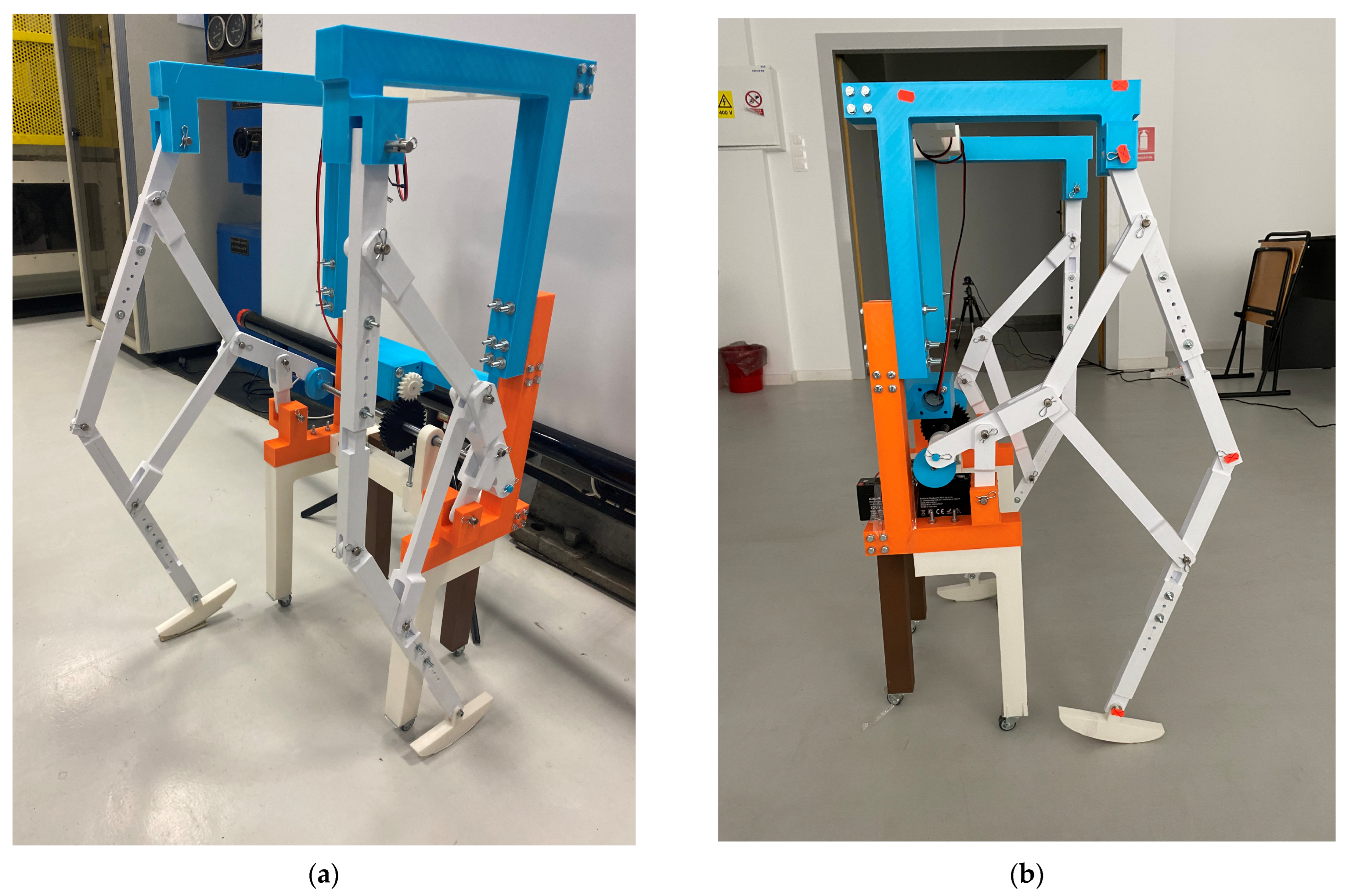
The experimental prototype and setup used for CONTEMPLAS-based motion analysis is shown in Figure 19 (see also Video S2 in the Supplementary Material). The prototype was first evaluated in a bench configuration to verify repeatability and marker visibility, and then tested on the dedicated rig under controlled motion cycles for high-speed video acquisition.

6.3. Experimental Motion Capture Using CONTEMPLAS and High-Speed Cameras

Experimental validation of the mechanism motion was performed by video-based kinematic analysis using CONTEMPLAS motion analysis software version 2025 and high-speed video cameras. The measurement setup consisted of two cameras arranged to provide full visibility of the leg motion in the sagittal plane, while minimizing perspective errors and occlusions in joint areas. Uniform illumination was used to ensure stable marker detection and reduce motion blur at high frame rates.

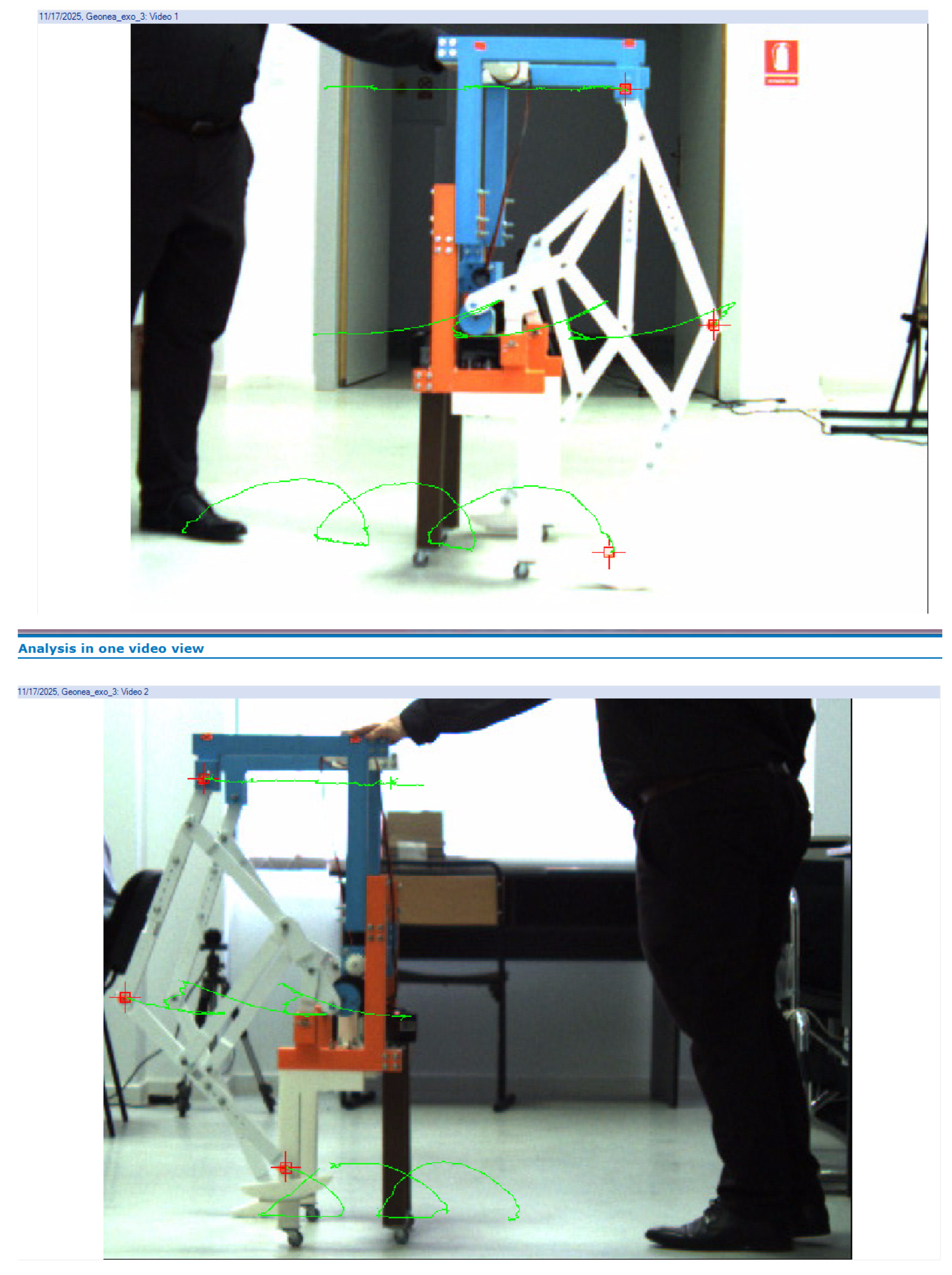
A calibration procedure was performed prior to acquisition using a standard calibration target, enabling transformation of image coordinates into real-world coordinates. A global reference frame was defined consistently with the simulation coordinate system (horizontal X, vertical Y), allowing direct comparison between experimental trajectories and ADAMS outputs. Physical markers (high-contrast circular targets) were attached to key points of the mechanism, including the hip joint center, knee joint center, and the distal point M (tracked as the foot point). The marker corresponding to point M was used to extract the horizontal and vertical displacement histories, consistent with MARKER_108 outputs used in the simulation results.

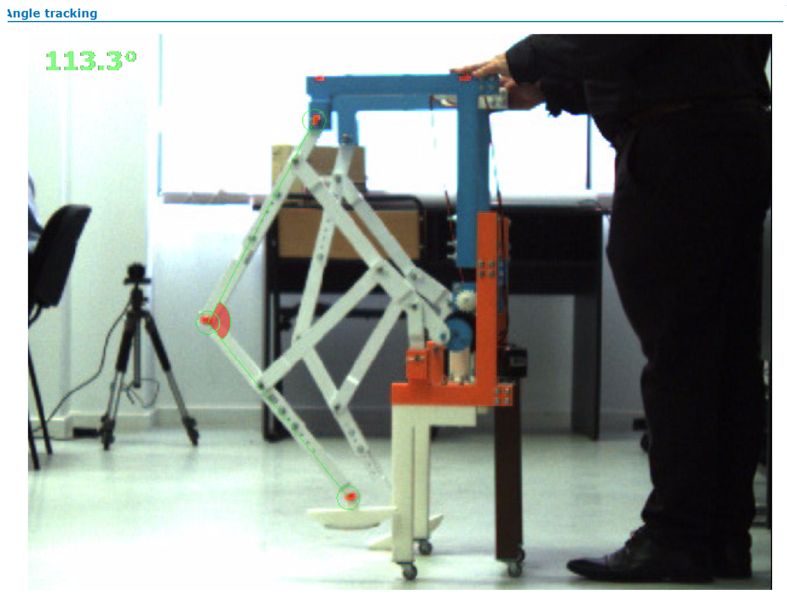
Video-based motion capture was carried out using the CONTEMPLAS software by tracking high-contrast markers attached to key points of the mechanism. Figure 20 illustrates a representative tracking frame, where the detected marker positions are superimposed on the recorded high-speed video and the corresponding trajectories are reconstructed in the sagittal plane. The tracked points included the hip and knee joint regions, as well as the distal point M (foot point), enabling the extraction of X(t) and Y(t) displacement histories and the subsequent computation of joint angles from relative marker motion.

To ensure repeatability, marker visibility was checked over the entire cycle and the acquisition was performed under controlled illumination and camera placement. The exported marker trajectories were then post-processed to obtain cycle-averaged kinematics and to quantify the agreement with the ADAMS simulations through RMSE-based metrics (Section 6.5).

6.4. Measurement Protocol and Extracted Quantities

For each test case, the mechanism was actuated using a DC geared motor (SG27-B round gear motor) [38] as the input drive, providing a repeatable motion profile over a 2.6 s interval corresponding to three consecutive cycles. Video acquisition was performed at 300 frames per second (fps), with the exposure time set sufficiently short to avoid motion blur and to ensure robust marker detection throughout the cycle. The following kinematic quantities were extracted from the tracked marker trajectories:

○

planar trajectory of the foot point M, expressed as X_M(t) and Y_M(t);

○

hip and knee rotation angles obtained either directly (if angular tracking was configured) or computed from the relative marker positions on adjacent links;

○

cycle timing indicators (period, stance/swing-like intervals), obtained from the periodic features of Y_M(t) and/or joint angle profiles.

To reduce measurement noise while preserving the relevant kinematic content, the recorded marker trajectories were smoothed using a low-pass Butterworth filter (cut-off frequency 6 Hz), applied consistently to all exported X(t) and Y(t) signals. The same post-processing workflow was used across all scenarios to ensure comparability.

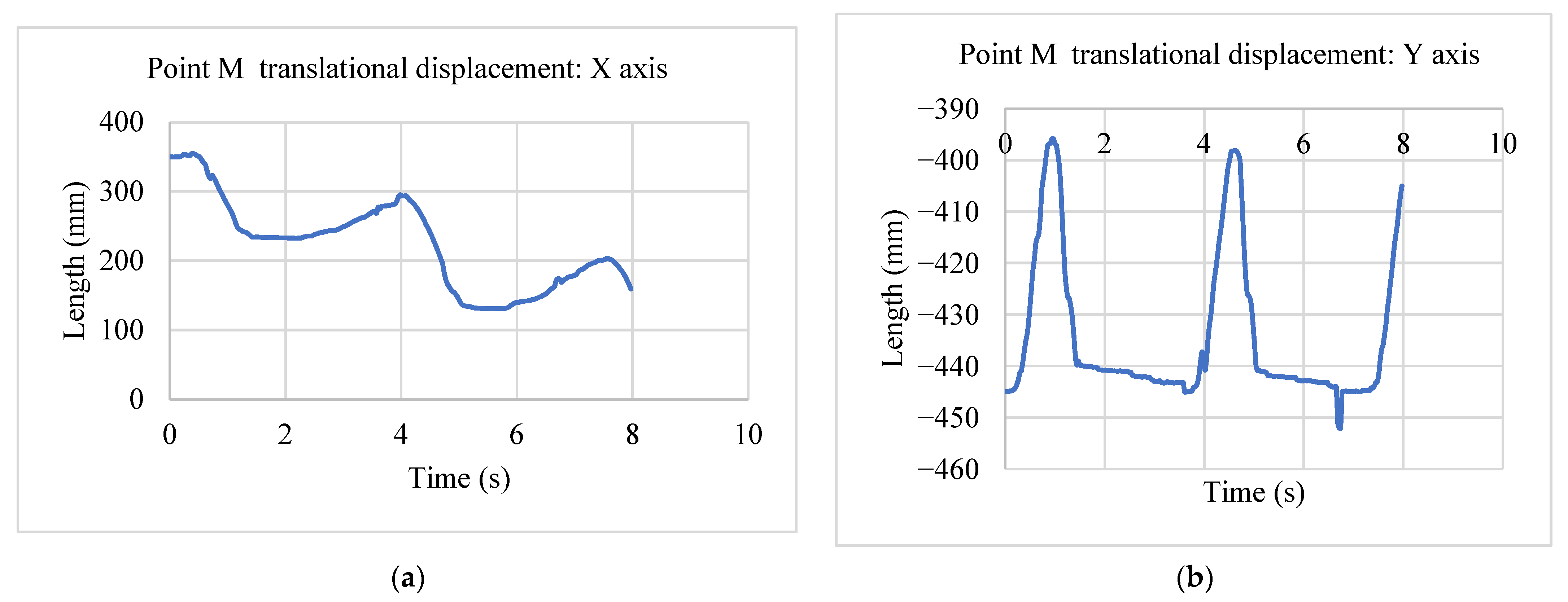
Figure 21 reports the experimentally measured displacement histories of point M (foot point) obtained from the CONTEMPLAS marker tracking. The horizontal displacement X_M(t) (Figure 21a) shows a repeatable gait-like pattern over the recorded interval (0–8 s), with values ranging approximately from ~130 mm to ~350 mm (ΔX ≈ 220 mm). The curve exhibits a gradual decrease followed by a recovery, which is consistent with alternating stance-like and swing-like phases in the fixed-frame experimental test.

The vertical displacement Y_M(t), (Figure 21b) remains bounded between approximately −455 mm and −395 mm (ΔY ≈ 60 mm) and displays distinct periodic peaks (at about 0.9 s and 4.6 s), corresponding to the foot clearance phase. From the timing of consecutive peaks, the cycle period is approximately 3.7 s, confirming stable periodic motion. These experimental trajectories provide the reference dataset used in the subsequent validation step, where the agreement between measured and simulated kinematics is quantified through RMSE-based metrics (Section 6.5).

Overall, the measured X_M(t) and Y_M(t) trends are consistent with the ovoid end-point motion predicted by the ADAMS model, supporting the validity of the simulation-driven design.

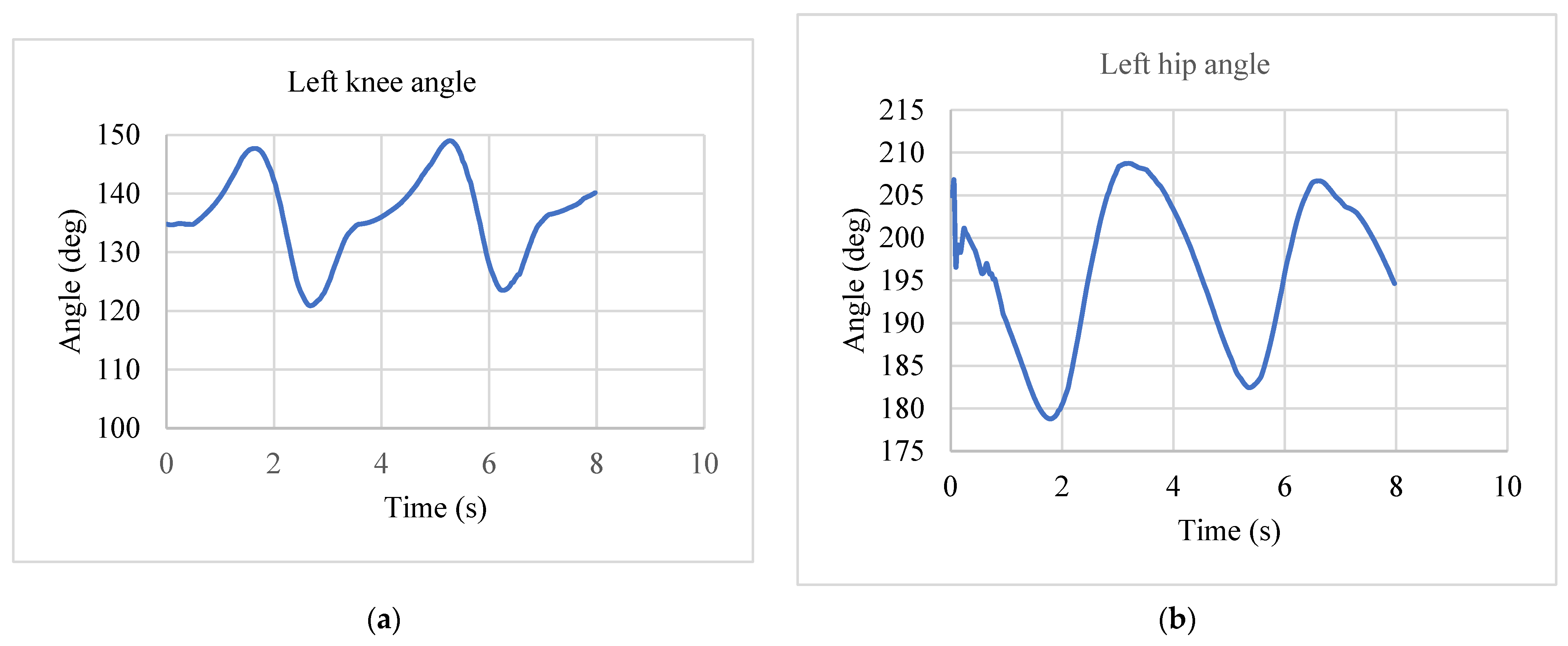
In addition to the end-point displacements, the joint kinematics were also quantified from the tracked marker trajectories (Figure 22). Using the planar assumption (sagittal-plane motion), the hip and knee rotation angles were computed from the relative orientation of adjacent link segments defined by marker pairs placed on the corresponding rigid bodies. This processing provides time histories θ_H(t) and θ_K(t) that can be directly compared to the ADAMS joint-angle outputs under identical operating conditions.

The measured angle profiles are periodic and synchronized with the displacement histories of point M. The knee angle exhibits a larger excursion (flexion peak during the clearance phase), while the hip angle shows a smoother, lower-amplitude modulation that drives the global limb swing. The cycle-to-cycle repeatability observed in the measured θ_H(t) and θ_K(t) confirms stable prototype operation and supports the subsequent quantitative validation against simulation results using RMSE-based metrics (Section 6.5).

6.5. Comparison with ADAMS Simulations

The experimentally measured trajectories and joint angle histories were compared to the corresponding ADAMS simulation outputs for the same scenario definitions. The comparison focused on (i) the overall shape of the foot trajectory (ovoid pattern and step-like progression), (ii) peak-to-peak amplitudes in X_M and Y_M, and (iii) timing consistency (cycle period and phase relationship between hip and knee motion).

Quantitative agreement was evaluated using standard metrics such as the root-mean-square error (RMSE) and maximum absolute deviation:

For a continuous signal evaluated over a time interval [0, T]:

$$\begin{gathered} {\mathrm{R}\mathrm{M}\mathrm{S}\mathrm{E}}_X=\sqrt{{\displaystyle \frac{1}{T}}{\int }_0^T{\left(X^{\mathrm{e}\mathrm{x}\mathrm{p}}\left(t\right)-X^{\mathrm{s}\mathrm{i}\mathrm{m}}\left(t\right)\right)}^2\hspace{0.17em}dt} \\ {\mathrm{R}\mathrm{M}\mathrm{S}\mathrm{E}}_Y=\sqrt{{\displaystyle \frac{1}{T}}{\int }_0^T{\left(Y^{\mathrm{e}\mathrm{x}\mathrm{p}}\left(t\right)-Y^{\mathrm{s}\mathrm{i}\mathrm{m}}\left(t\right)\right)}^2\hspace{0.17em}dt} \end{gathered}$$

(14)

For sampled data with N samples:

$$\begin{gathered} {\mathrm{R}\mathrm{M}\mathrm{S}\mathrm{E}}_X=\sqrt{{\displaystyle \frac{1}{N}}\sum _{i=1}^N{\left(X_i^{\mathrm{e}\mathrm{x}\mathrm{p}}-X_i^{\mathrm{s}\mathrm{i}\mathrm{m}}\right)}^2} \\ {\mathrm{R}\mathrm{M}\mathrm{S}\mathrm{E}}_Y=\sqrt{{\displaystyle \frac{1}{N}}\sum _{i=1}^N{\left(Y_i^{\mathrm{e}\mathrm{x}\mathrm{p}}-Y_i^{\mathrm{s}\mathrm{i}\mathrm{m}}\right)}^2} \\ {\mathrm{R}\mathrm{M}\mathrm{S}\mathrm{E}}_{2\mathrm{D}}=\sqrt{{\displaystyle \frac{1}{N}}\sum _{i=1}^N\left[{\left(X_i^{\mathrm{e}\mathrm{x}\mathrm{p}}-X_i^{\mathrm{s}\mathrm{i}\mathrm{m}}\right)}^2+{\left(Y_i^{\mathrm{e}\mathrm{x}\mathrm{p}}-Y_i^{\mathrm{s}\mathrm{i}\mathrm{m}}\right)}^2\right]} \end{gathered}$$

(15)

When the trajectory error is evaluated jointly in the (X, Y) plane:

$${\mathrm{R}\mathrm{M}\mathrm{S}\mathrm{E}}_{2\mathrm{D}}=\sqrt{{\displaystyle \frac{1}{N}}\sum _{i=1}^N\left[{\left(X_i^{\mathrm{e}\mathrm{x}\mathrm{p}}-X_i^{\mathrm{s}\mathrm{i}\mathrm{m}}\right)}^2+{\left(Y_i^{\mathrm{e}\mathrm{x}\mathrm{p}}-Y_i^{\mathrm{s}\mathrm{i}\mathrm{m}}\right)}^2\right]}$$

(16)

Quantitative agreement between the CONTEMPLAS measurements and the MSC ADAMS outputs was assessed over a representative gait-like cycle. Because experimental and simulated signals may exhibit slight timing differences, the trajectories were time-normalized to a 0–100% cycle and resampled to N = 101 points before comparison. The knee angle measured experimentally was converted to flexion as θ_K = 180° − θ_K,exp, while the hip angle was referenced to the neutral posture as θ_H = θ_H,exp − 180° to match the ADAMS joint rotation conventions. The resulting RMSE values were 28.1 mm for X_M(t) and 35.7 mm for Y_M(t), while the joint-angle RMSE reached 13.4° for the hip and 6.35° for the knee. Minor discrepancies are primarily attributed to differences between the experimental angle definition (marker-based reconstruction) and the ideal revolute-joint definition used in the multibody model, as well as small timing shifts compensated by cycle normalization. Overall, the measured trajectories preserve the same periodic structure and amplitude hierarchy predicted by ADAMS, confirming that the simulation-driven model provides a valid representation of the prototype kinematics.

In addition, peak values of the hip and knee angles per cycle were compared to verify that the prototype reproduces the expected joint coordination identified in the fixed-frame and progression simulations.

7. Discussion

The results support an integrated design workflow in which multibody dynamics is used not only to assess kinematic suitability but also to generate representative operational loads for structural design. The selected Chebyshev-driven pantograph architecture produces a repeatable, gait-relevant end-point motion, with synchronized hip–knee coordination across all investigated scenarios (fixed-frame, ramp, stair ascent, and inclined-plane walking). Importantly, the ADAMS simulations provide joint reaction force histories that are physically consistent with task difficulty: the hip joint generally represents the dominant load path, while the knee joint exhibits lower but clearly cyclic force peaks. This trend is coherent with the mechanism’s role of transferring support and propulsion loads through the proximal joint during stance and uphill/step negotiation.

From a structural standpoint, the surrogate-based ANSYS optimization demonstrates that meaningful mass reduction can be achieved while respecting stiffness and strength constraints when the design space is parameterized through manufacturable geometric variables. The response surfaces highlight a clear mass–stiffness–strength coupling: thickness-related parameters and the global width parameter (P1 and the extrusion-related dimensions) strongly affect mass and deformation, while fillet radii primarily influence stress concentrations. By combining DoE sampling, response surface surrogates, and MOGA, the optimization converges to feasible candidates that satisfy P7 ≤ 0.2 mm and P8 ≤ 50 MPa while minimizing mass, resulting in a lightweight configuration suitable for rapid prototyping and iterative testing.

The experimental campaign complements the simulation results by providing measured point-M trajectories and joint-angle histories obtained from CONTEMPLAS high-speed video tracking. The measured X_M(t) and Y_M(t) histories preserve the expected periodic features (clearance peaks in Y_M and cycle-to-cycle repeatability), supporting the qualitative validity of the ADAMS-predicted ovoid end-point motion. In addition, the experimentally reconstructed hip and knee angles exhibit the expected amplitude hierarchy (larger knee excursion during clearance), consistent with the simulated coordination. The agreement is quantified in Section 6.5 through RMSE-based metrics, enabling an objective validation of the simulation-driven design approach.

Several limitations should be acknowledged. First, the mechanism is modeled as planar and primarily rigid, which neglects out-of-plane dynamics and compliance in joints and links that may become relevant under higher loads or faster actuation. Second, the ground contact model and environmental interaction in ADAMS represent simplified contact assumptions, which can influence peak force predictions. Third, the rapid prototype manufactured by 3D printing is intended for kinematic validation rather than final load-bearing performance; material anisotropy and joint wear can affect the measured trajectories. Future work will address these aspects by extending the model to include compliant elements and joint clearances, performing fatigue-oriented structural assessment for metallic or composite implementations, and developing closed-loop control strategies with human-in-the-loop experiments under standardized gait rehabilitation protocols.

A further limitation stems from the anatomical simplification adopted in the present mechanism. The human lower limb does not behave as an ideal serial chain with perfectly fixed hip and knee axes; in particular, the knee exhibits polycentric behavior, and the effective hip center may vary with pelvic motion. The proposed exoskeleton approximates these biomechanics by means of fixed revolute joints in a planar architecture, which is acceptable only as a first engineering approximation for controlled sagittal-plane rehabilitation scenarios. A more anatomically compatible implementation would require passive self-alignment degrees of freedom, compliant interfaces [39,40], or dedicated polycentric joint mechanisms, and this constitutes an important direction for future work.

8. Conclusions

This paper presented a planar lower-limb rehabilitation exoskeleton leg based on a pantograph-derived architecture driven by a Chebyshev Lambda linkage and validated through an integrated simulation–optimization–experiment workflow. Multibody simulations in MSC ADAMS demonstrated gait-relevant end-point motion and provided representative joint reaction forces under multiple scenarios (fixed-frame, ramp progression, stair ascent, and inclined-plane walking). These loads were transferred to ANSYS Workbench, where a surrogate-based optimization (DoE + response surfaces + MOGA) enabled mass minimization under stiffness and strength constraints, yielding a lightweight feasible design for rapid prototyping.

A rapid prototype was manufactured by 3D printing and experimentally evaluated using CONTEMPLAS high-speed video tracking. The measured point-M trajectories and joint-angle histories confirmed stable periodic motion and qualitative consistency with the simulated kinematics. Quantitative comparison is formulated through RMSE-based metrics, providing an objective basis for validating the simulation-driven design methodology. Overall, the proposed workflow supports fast iteration of linkage-based exoskeleton mechanisms by linking dynamic load prediction, manufacturable structural optimization, and video-based experimental verification.

The present results establish mechanism-level feasibility, representative joint-loading conditions, and prototype-motion consistency, but they do not yet constitute a full validation of biomechanical compatibility or clinical assistance efficacy in human subjects.

9. Patents

Geonea, I.D.; Dumitru, N.; Dumitru, S.; Copiluși, P.C.; Ciurezu-Gherghe, L. Exoskeleton meant for human walking assistance and rehabilitation. Romanian Patent RO134430A1, 30 September 2020 [32].

Geonea, I.D.; Tarnita, D. Modular exoskeleton with applications in human lower-limb locomotor recovery. Romanian Patent RO132701B1, 30 October 2024 [33].

References

1. Flor-Unda, O.; Arcos-Reina, R.; Toapanta, C.; Villao, F.; Bustos-Estrella, A.; Suntaxi, C.; Palacios-Cabrera, H. Challenges in the Development of Exoskeletons for People with Disabilities. Technologies 2025, 13, 291. [Google Scholar] [CrossRef]
2. Hasan, S.; Alam, N. Comprehensive Comparative Analysis of Lower Limb Exoskeleton Research: Control, Design, and Application. Actuators 2025, 14, 342. [Google Scholar] [CrossRef]
3. Lin, W.; Dong, H.; Gao, Y.; Wang, W.; Long, Y.; He, L.; Mao, X.; Wu, D.; Dong, W. A Systematic Review of Locomotion Assistance Exoskeletons: Prototype Development and Technical Challenges. Technologies 2025, 13, 69. [Google Scholar] [CrossRef]
4. Cenciarini, M.; Dollar, A.M. Biomechanical Considerations in the Design of Lower Limb Exoskeletons. In Proceedings of the 2011 IEEE International Conference on Rehabilitation Robotics (ICORR), Zurich, Switzerland, 29 June–1 July 2011; pp. 1–6. [Google Scholar] [CrossRef]
5. Thalman, C.; Artemiadis, P. A Review of Soft Wearable Robots That Provide Active Assistance: Trends, Common Actuation Methods, Fabrication, and Applications. Wearable Technol. 2020, 1, e3. [Google Scholar] [CrossRef]
6. Sanchez-Villamañan, M.D.C.; Gonzalez-Vargas, J.; Torricelli, D.; Moreno, J.C.; Pons, J.L. Compliant Lower Limb Exoskeletons: A Comprehensive Review on Mechanical Design Principles. J. Neuroeng. Rehabil. 2019, 16, 55. [Google Scholar] [CrossRef]
7. Lu, J.; Lv, X.; Liu, J.; Liu, H.; Huang, T. Fully Flexible Wearable Pouch Pneumatic Artificial Muscle Based on Asymmetric Expansion. Chin. J. Mech. Eng. 2026, 39, 100085. [Google Scholar] [CrossRef]
8. Cho, Y.; Kim, W.; Park, H.; Kim, J.; Na, Y. Bidirectional Double-Spring Pneumatic Artificial Muscle with Inductive Self-Sensing. IEEE Robot. Autom. Lett. 2023, 8, 8160–8167. [Google Scholar] [CrossRef]
9. Bettella, F.; Tortora, S.; Menegatti, E.; Petrone, N.; Del Felice, A. A Scoping Review on Lower Limb Exoskeleton Actuation’s Description and Characteristics. Robotica 2025, 43, 1572–1589. [Google Scholar] [CrossRef]
10. Xu, X.; Chen, C.; Sun, Z.; Xian, W.; Ma, L.; Liu, Y. Research on Control Strategy of Lower Limb Exoskeleton Robots: A Review. Sensors 2026, 26, 355. [Google Scholar] [CrossRef]
11. Song, Z.; Zhao, P.; Wu, X.; Yang, R.; Gao, X. An Active Control Method for a Lower Limb Rehabilitation Robot with Human Motion Intention Recognition. Sensors 2025, 25, 713. [Google Scholar] [CrossRef]
12. Zhang, P.; Gao, X.; Miao, M.; Zhao, P. Design and Control of a Lower Limb Rehabilitation Robot Based on Human Motion Intention Recognition with Multi-Source Sensor Information. Machines 2022, 10, 1125. [Google Scholar] [CrossRef]
13. Rosales-Luengas, Y.; Espinosa-Espejel, K.I.; Lopéz-Gutiérrez, R.; Salazar, S.; Lozano, R. Lower Limb Exoskeleton for Rehabilitation with Flexible Joints and Movement Routines Commanded by Electromyography and Baropodometry Sensors. Sensors 2023, 23, 5252. [Google Scholar] [CrossRef]
14. Guo, Y.; He, M.; Tong, X.; Zhang, M.; Huang, L. Research on the Motion Control Strategy of a Lower-Limb Exoskeleton Rehabilitation Robot Using the Twin Delayed Deep Deterministic Policy Gradient Algorithm. Sensors 2024, 24, 6014. [Google Scholar] [CrossRef] [PubMed]
15. Lee, J.; Huber, M.E.; Hogan, N. Gait Entrainment to Torque Pulses from a Hip Exoskeleton Robot. IEEE Trans. Neural Syst. Rehabil. Eng. 2022, 30, 656–667. [Google Scholar] [CrossRef] [PubMed]
16. Khan, N.A.; Jamwal, P.K.; Hussain, F.; Spratford, W.; Hussain, S. Quantum Enhanced Transformer Network for Learning Transactive Energy During Physical Human-Robot Interaction. IEEE Trans. Hum. -Mach. Syst. 2025, 55, 930–939. [Google Scholar] [CrossRef]
17. Khan, N.A.; Jamwal, P.K.; Hussain, F.; Ghayesh, M.H.; Hussain, S. Reinforcement Learning-Driven Path Generation for Ankle Rehabilitation Robot Using Musculoskeletal-Informed Energy Optimization. IEEE Trans. Neural Syst. Rehabil. Eng. 2025, 33, 1774–1784. [Google Scholar] [CrossRef]
18. Khan, N.A.; Hussain, S.; Spratford, W.; Goecke, R.; Kotecha, K.; Jamwal, P.K. Deep Learning-Driven Analysis of a Six-Bar Mechanism for Personalized Gait Rehabilitation. J. Comput. Inf. Sci. Eng. 2025, 25, 011001. [Google Scholar] [CrossRef]
19. Yao, Y.; Shao, D.; Tarabini, M.; Moezi, S.A.; Li, K.; Saccomandi, P. Advancements in Sensor Technologies and Control Strategies for Lower-Limb Rehabilitation Exoskeletons: A Comprehensive Review. Micromachines 2024, 15, 489. [Google Scholar] [CrossRef]
20. Huo, C.; Shao, G.; Chen, T.; Li, W.; Wang, J.; Xie, H.; Wang, Y.; Li, Z.; Zheng, P.; Li, L.; et al. Effectiveness of unilateral lower-limb exoskeleton robot on balance and gait recovery and neuroplasticity in patients with subacute stroke: A randomized controlled trial. J. Neuroeng. Rehabil. 2024, 21, 213. [Google Scholar] [CrossRef]
21. Zhang, Y.; Zhao, W.; Wan, C.; Wu, X.; Huang, J.; Wang, X.; Huang, G.; Ding, W.; Chen, Y.; Yang, J.; et al. Exoskeleton Rehabilitation Robot Training for Balance and Lower Limb Function in Sub-Acute Stroke Patients: A Pilot, Randomized Controlled Trial. J. Neuroeng. Rehabil. 2024, 21, 98. [Google Scholar] [CrossRef]
22. Louie, D.R.; Mortenson, W.B.; Durocher, M.; Schneeberg, A.; Teasell, R.; Yao, J.; Eng, J.J. Efficacy of an Exoskeleton-Based Physical Therapy Program for Non-Ambulatory Patients during Subacute Stroke Rehabilitation: A Randomized Controlled Trial. J. Neuroeng. Rehabil. 2021, 18, 149. [Google Scholar] [CrossRef] [PubMed]
23. Wall, A.; Borg, J.; Vreede, K.; Palmcrantz, S. A Randomized Controlled Study Incorporating an Electromechanical Gait Machine, the Hybrid Assistive Limb, in Gait Training of Patients with Severe Limitations in Walking in the Subacute Phase after Stroke. PLoS ONE 2020, 15, e0229707. [Google Scholar] [CrossRef]
24. Hsu, T.H.; Tsai, C.L.; Chi, J.Y.; Hsu, C.Y.; Lin, Y.N. Effects of Wearable Exoskeletons on Post-Stroke Gait Rehabilitation: A Systematic Review and Meta-Analysis. Ann. Phys. Rehabil. Med. 2023, 66, 101674. [Google Scholar] [CrossRef]
25. Rodríguez-Fernández, A.; Lobo-Prat, J.; Font-Llagunes, J.M. Systematic Review on Wearable Lower-Limb Exoskeletons for Gait Training in Neuromuscular Impairments. J. Neuroeng. Rehabil. 2021, 18, 22. [Google Scholar] [CrossRef]
26. Liu, S.; Chen, F.; Yin, J.; Wang, G.; Yang, L. Comparative Efficacy of Robotic Exoskeleton and Conventional Gait Training in Patients with Spinal Cord Injury: A Meta-Analysis of Randomized Controlled Trials. J. Neuroeng. Rehabil. 2025, 22, 121. [Google Scholar] [CrossRef]
27. Yoo, H.-J.; Bae, C.R.; Jeong, H.; Ko, M.-H.; Kang, Y.-K.; Pyun, S.-B. Clinical efficacy of overground powered exoskeleton for gait training in patients with subacute stroke: A randomized controlled pilot trial. Medicine 2023, 102, e32761. [Google Scholar] [CrossRef] [PubMed]
28. Guo, S.; Yang, Y.; Wang, M.; Wang, D.; Zhang, Y.; Wang, Q.; Deng, Y. Effects of an Exoskeleton Robot on Motor Function in Patients with Spinal Cord Injuries: A Systematic Review and Meta-Analysis. Syst. Rev. 2025, 14, 218. [Google Scholar] [CrossRef]
29. Shi, D.; Zhang, W.; Zhang, W.; Ding, X. A Review on Lower Limb Rehabilitation Exoskeleton Robots. Chin. J. Mech. Eng. 2019, 32, 74. [Google Scholar] [CrossRef]
30. Chen, C.F.; Du, Z.J.; He, L.; Shi, Y.J.; Wang, J.Q.; Xu, G.Q.; Zhang, Y.; Wu, D.M.; Dong, W. Development and Hybrid Control of an Electrically Actuated Lower Limb Exoskeleton for Motion Assistance. IEEE Access 2019, 7, 169107–169122. [Google Scholar] [CrossRef]
31. Geonea, I.; Copilusi, C.; Tarnita, D. Development of a New Leg Mechanism for Exoskeleton Robots: Structural Synthesis, Dynamic Analysis, and Prototype Implementation. In International Workshop IFToMM for Sustainable Development Goals; Springer Nature: Cham, Switzerland, 2025; pp. 310–318. [Google Scholar]