Model-Based Design of the 5-DoF Light Industrial Robot

Abstract

With the application and rapid development of light industrial robots, it is vital to accelerate the prototype design to fulfill the demands of shortening the robot’s production cycle, owing to rapid update iterations. Since the traditional design method cannot intuitively and efficiently check the deficiencies in the design preparation, the secondary design iterations will result in higher equipment costs, longer design cycles, and lower development efficiency. The MBD (model-based design), a full 3D (three-dimensional) design and manufacturing method, is proposed to swiftly finish the prototype design for solving the above problems. Firstly, the robot design preparation is completed with the design requirements to generate a robot 3D model. Secondly, several design methods are used: (i) the rapid prototyping, which includes the joint component verification and selection to further optimize the 3D model; (ii) the robot kinematics algorithm, which provides a theoretical foundation for the 3D model design; (iii) the robot kinematics simulation, which verifies the correctness of the kinematics algorithm. Finally, the feasibility of the MBD is verified by the robot prototype and the motion control system test. Taking the MBD to design a 5-DoF (five-degrees-of-freedom) robot as an example, the joint verification and selection are finished quickly and accurately to build the robot prototype without the need for secondary design processing, and the kinematic algorithm verified by the co-simulation platform can be used directly in the actual motion control of the robot prototype, which accelerates the development of the robot motion control system.

1. Introduction

With the advancement of computer technology, CAD/CAM and digital twin technologies have been widely applied in robotic system modeling and control. However, CAD/CAM is mainly used in early design, while digital twins are employed after prototype fabrication for simulation and control [1,2,3]. This separation leads to low integration between design and control, making it difficult to detect flaws early and often resulting in costly secondary design iterations, prolonged cycles, and reduced development efficiency [4,5]. To bridge this gap, this paper proposes an integrated model-based design (MBD) approach that unifies design, simulation, and control. The method is demonstrated using a PRRRR five-axis robot to standardize prototype design and motion control development, effectively shortening the development cycle and supporting control optimization.

The designed five-axis PRRRR (prismatic–revolute–revolute–revolute–revolute) robot is a lightweight industrial robot, which has the advantages of lightweight, high mobility, and high precision, such as the UR cooperative robot [6,7,8] and Kuka robot [9,10,11]. The process of the MBD of the robot follows these steps: Firstly, according to the related robot design requirements, the robot design preparation is completed to generate a robot 3D model in the early stage of the robot MBD, which includes both the robot structure design and the robot 3D model design. Secondly, several design methods are adopted in the process of the MBD of the robot: (i) the rapid prototyping, which includes the joint component verification and selection of the robot to further optimize the robot 3D model by the robot Adams kinematics model; (ii) the robot kinematics algorithm, which includes kinematics analysis and trajectory planning, for realizing the motion control of the robot to provide a theoretical basis for the robot 3D model design and prove the reasonability of the motion control of the robot by the generated robot mathematical model; (iii) the robot kinematics simulation, which consists of building the co-simulation platform of Matlab 2018b and Vrep Edu and the simulation verification, completed by the robot urdf model to verify whether the robot can complete the given task according to the planned trajectory and the correctness of the robot kinematics algorithm. Finally, the correctness of the trajectory planning algorithm and the feasibility of the MBD of the robot are verified by the generation output of the robot prototype and the test of the developed motion control system. The design flow chart of the robot is shown in Figure 1.

This 3D modeling method, including the robot hardware, software, simulation, and algorithm, is based on MBD, which allows for analysis of the robot during the early design to effectively correct the defects, enhance the efficiency of the robot design, and reduce the development costs [12].

Many institutions at home and abroad have achieved good results in product design using the MBD method, which has overwhelmingly shortened the design cycle [13]. Researchers have found that the whole process of the product design cycle can be optimized using computer-aided design to create a detailed list of the future design indexes of products and perform the simulation, algorithm, and control tests according to research and design parameters and design requirements. This MBD system has achieved the first and greatest success in the fields of automobiles and aerospace. Saurabh Mahapatrash developed a hybrid electric vehicle system using the MBD, which can effectively help automotive engineers design electric drives [14]. Airbus employed the MBD to model and control the fuel system of the Airbus A380, greatly accelerating the coordinated development of various departments and completing the design of the fuel management system months in advance without additional manpower [15]. Building on these mature applications, several innovative extensions of MBD have been developed to address the unique challenges of reconfigurable robots: morphological templates enable rapid design variations, including serial/parallel joint switching configurations [16]; configuration-aware code generation automatically optimizes the control strategy for each topological variation [17]; and an automated documentation system ensures that the entire design process complies with industrial safety standards [18]. These advances specifically address the dynamic reconfiguration requirements and real-time control challenges inherent in modern robotic systems while retaining the proven advantages of the MBD approach.

The successful application of the MBD method in the automotive and aerospace industries has inspired advancements in robot control. Researchers, both domestically and internationally, are beginning to explore the use of the MBD approach to design control systems for robots. Alex Kai-Yuan Lo completed the design and evaluation of an active waist monkey robot using the MBD method, which can perform continuous braid movement on a swinging rod [19]. However, it is essential to build a simulation platform for the active waist monkey robot to verify the control algorithm.

Daniel employed the MBD method with the co-simulation platform of Inventor and Simulink to build the motion simulation and develop the control algorithm for the snake-like robot [20]. Beyond these examples, MBD has proven particularly valuable for reconfigurable robot design, as evidenced by recent work on origami-inspired metamorphic mechanisms that demonstrate remarkable kinematic adaptability through integrated 8R, 6R, and 4R configurations [21].

However, the developed control algorithm was not applied to a real prototype of the robot. Therefore, this paper proposed a general method of the MBD of a 5-Dof light industrial robot, including the robot design preparation, the robot design methods, and the robot generation output, which helps rapidly build the robot prototype by quickly and accurately completing the joint verification and selection without the need for secondary design processing. It is reasonable that the kinematic algorithm based on the robot 3D model verified by the co-simulation platform can be directly used in the actual motion control of the robot prototype, which accelerates the development of the robot motion control system.

This paper is organized as follows: Section 2 introduces the robot design preparation, which includes the robot structure design and the robot 3D model design. In Section 3, the robot design methods are introduced: (i) the rapid prototyping, which includes the joint component verification and selection of the robot; (ii) the robot kinematics algorithm, which includes kinematics analysis consisting of the establishment of the coordinate system, the forward kinematic analysis, the inverse kinematic analysis, and trajectory planning consisting of the joint space trajectory planning and the trajectory planning of Cartesian space; (iii) the robot kinematics simulation, which includes the co-simulation platform of Matlab 2018b and Vrep Edu, simulation verification of joint space trajectory planning, and simulation verification of Cartesian space trajectory planning. Section 4 introduces the robot prototype, the robot motion control system, and the test. In the last section, the conclusion and further supplementary work of this paper are discussed.

2. MBD: Robot Design Preparation

To quickly design the robot prototype using the MBD, it is necessary to complete the robot design preparation, including the structure design and 3D model design, in the early stage according to the related robot design requirements.

2.1. Robot Structure Design

Given that the robot is commonly required to perform welding tasks at multiple stations in the automatic welding production line, the structure of using a linear sliding table as a prismatic joint instead of a revolute joint can overwhelmingly expand the robot’s working space. This design ensures that the robot can efficiently complete welding tasks at various stations. The structure of the industrial robot designed in this paper is determined to be PRRRR type, which consists of one prismatic joint and four revolute joints. The robot structure is shown in Figure 2.

2.2. Robot 3D Model Design

The welding task requires high repetitive positioning accuracy for the robot’s end effector. The revolute joint will adapt the joint module connecting and driving the manipulator, which includes two encoders and a frameless direct drive motor to ensure sufficient repetitive positioning accuracy to complete the welding task.

At the same time, the welding task also requires the robot to operate smoothly while ensuring that the joint load is sufficient. Firstly, the RISllZ-14 joint module is selected as the drive component of the revolute joint 5. The material of connecting arm 1 is an aluminum alloy. Then, the RISlZ-14 joint module is selected as the drive component of the revolute joint 4, and the material of connecting arm 2 is an aluminum alloy. Similarly, the RISllZ-17 joint module is selected as the drive component of the revolute joint 3 and revolute joint 2. Finally, the overall weight of the manipulator is obtained, and the linear slide table with enough load is selected.

The three-dimensional model of the robot is designed in SolidWorks 2019 software [22] according to the above requirements and is shown in Figure 3.

3. MBD: Robot Design Methods

3.1. MBD: Rapid Prototyping

To shorten the prototype design cycle and reduce the cost associated with secondary development, rapid prototyping using MBD is the most effective for robot design, which includes the joint components verification and selection of the robot. This approach has the benefit of allowing the robot’s 3D model to be immediately optimized using the robot’s kinematics model without the requirement for secondary design iterations.

3.1.1. Joint Components Verification

Before selecting the joint components, it is essential to analyze the output torque or force curve of each joint in the Adams 2019 software to ensure a reasonable selection [23].

The robot Adams kinematic model is generated by importing the 3D model of the robot into the Adams software, shown in Figure 4, which can provide the basis of physical movement to further optimize the 3D model according to the output torque or force curve of each joint.

Before starting the simulation, each part is renamed and material properties are added. Then, a revolute pair is added to each revolute joint, a moving pair is added to the prismatic joint, and other parts are fixed connections. Finally, the sine excitation drive is added to each joint, and the simulation is carried out.

The joint force or torque curve is generated by verification, which is also shown in Figure 5.

In Figure 5, the torque curves of joints 2–5 are shown from top to bottom. According to the curve analysis, the maximum force of joint 1 during motion is 123.23 N; the maximum torque of joint 5 during operation is 0.30 Nm; the maximum torque of joint 4 is 9.61 Nm; the maximum torque of joint 3 during operation is 21.43 Nm; the maximum torque of joint 2 is 33.96 Nm.

3.1.2. Joint Components Selection

According to the comparison between the maximum torque value of each joint and the average load torque in the parameters of the two types of joint modules in

Table 1. MBD: component parameter table.

Component	Output	Maximum Speed	Weight	Positioning Accuracy	Communication Protocol
RJSIIZ-14 joint module	13.5 (Nm)	47.5 (rpm)	1.0 (kg)	0.015 (°)	EtherCAT
RJSIIZ-17 joint module	49.0 (Nm)	35.0 (rpm)	1.9 (kg)
Linear slide table	367(N)	1.0 (m/s)	/	±0.005 (mm)

, it can be seen that RJSIIZ-14 joint modules are selected for joints 4 and 5, and RJSIIZ-17 joint modules are selected for joints 1 and 2 to complete a reasonable selection of joint components. At the same time, the total weight of the manipulator measured by SolidWorks is 9.72083 kg, and the selection of the slide table is completed within the horizontal load range of the linear slide table parameters in Table 1.

The reasonability of joint component selection was finally verified by the robot kinematics, and kinematics simulation was used for completing rapid prototyping. The component parameters are shown in Table 1, which includes the RJSIIZ-14 joint module parameter, the RJSIIZ-17 joint module parameter, and the linear slide table parameter.

Thus, compared with the traditional CAD/CAM design method, the joint verification and selection are completed quickly and accurately to generate the optimized 3D model of the robot by the MBD in the early stage of robot prototype design.

3.2. MBD: Robot Kinematics Algorithm

In order to control the MBD robot to complete a given task, it is critical to carry out kinematic analysis and trajectory planning for the robot’s 3D model design and demonstrate the reasonability of the motion control of the robot after the early stage of robot prototype design.

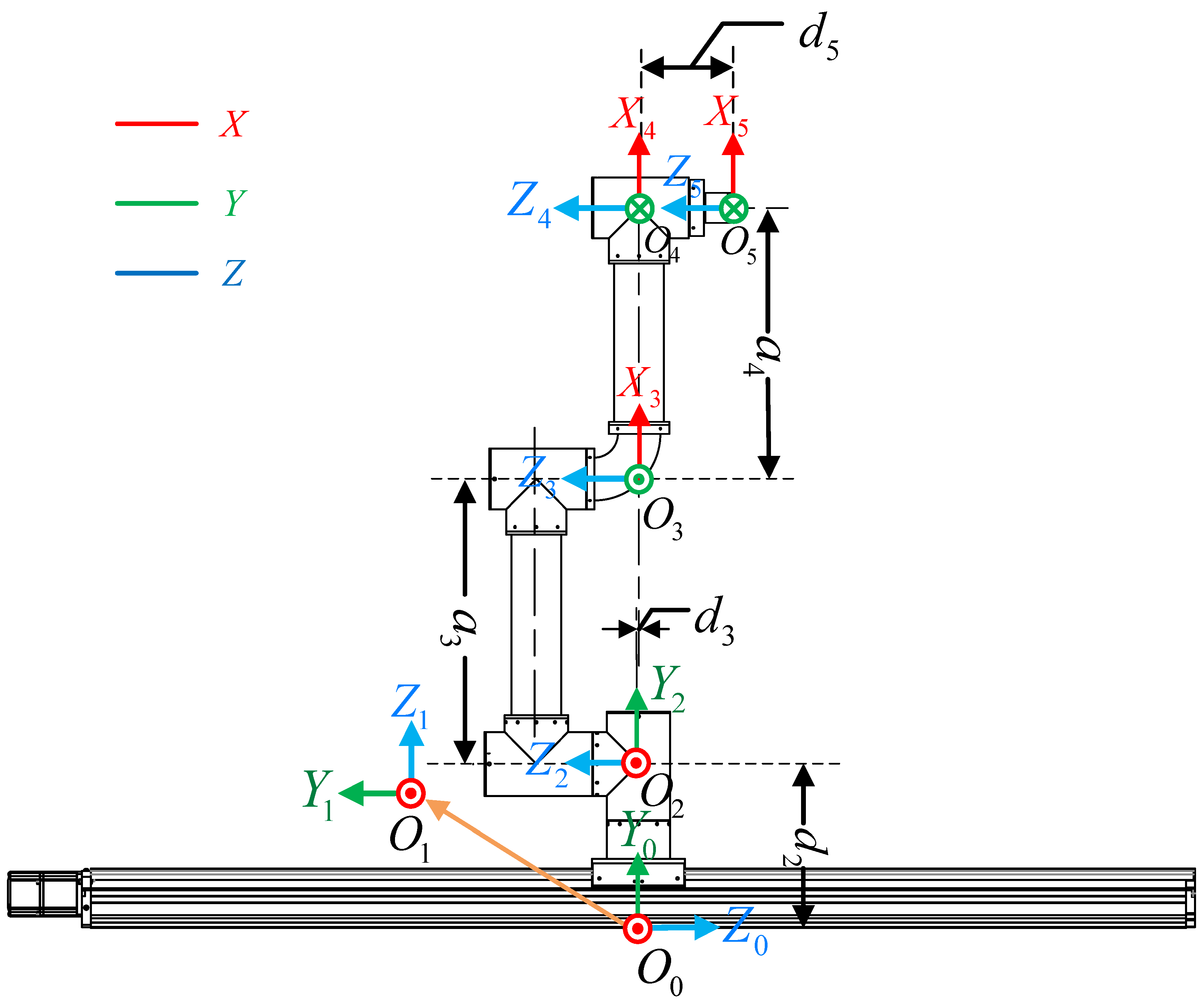
3.2.1. Kinematics Analysis

The robot kinematics analysis, which entails the establishment of the coordinate system, the forward kinematic analysis, and the inverse kinematic analysis, is the first step in realizing the digitization and programmability of the MBD robot. It also serves as a crucial foundation for confirming that the designed robot conforms to the robot kinematics principle.

• Establishment of the coordinate system

In robot kinematics analysis, the D-H (Denavit–Hartenberg) method is often used to establish the robot coordinate system. The D-H method includes the SD-H (standard Denavit–Hartenberg) method [24] and the MD-H (modified Denavit–Hartenberg) method [25]. The robot coordinate system established by the SD-H method is shown in Figure 6. A coordinate system is fixed on each link of the robot, and a 4 × 4 homogeneous transformation matrix, represented by ${\theta }_i$, $d_i$, $a_i,$ and ${\alpha }_i$ parameters, is used to describe the spatial relationship between two adjacent links. The position of the end effector relative to the base coordinate system is derived by sequential transformation to establish the kinematic equation of the robot.

According to the established robot coordinate system, the D-H parameters of the robot are shown in

Table 2. MBD: the robot D-H parameter table.

$\mathit{Joint} \mathit{i}$	${\mathit{\theta }}_{\mathit{i}} (\mathbf{deg})$	${\mathit{d}}_{\mathit{i}} \left(\mathbf{m}\mathbf{m}\right)$	${\mathit{a}}_{\mathit{i}} \left(\mathbf{m}\mathbf{m}\right)$	${\mathit{\alpha }}_{\mathit{i}} (\mathbf{deg})$
1	$\pi /2$	$d_1$	0	$\pi /2$
2	${\theta }_2$	209	0	$\pi /2$
3	${\theta }_3$	−5.89	379.5	0
4	${\theta }_4$	0	364	0
5	${\theta }_5$	−126.89	0	0

, which are measured in the SolidWorks 2019 software.

In the table, $i$ is the number of joints, and ${\theta }_i$, $d_i$, $a_i$, and ${\alpha }_i$ are link parameters of joint $i$. For example, ${\theta }_i$ is the rotation angle from $x_{i-1}$ to $x_i$ around axis $z_{i-1}$, $d_i$ is the moving distance from $x_{i-1}$ to $x_i$ along axis $z_i$,$a_i$ is the moving distance from $z_{i-1}$ to $z_i$ along axis $x_i$, and ${\alpha }_i$ is the rotation angle from $z_{i-1}$ to $z_i$ around axis $x_i$.

B.

Forward kinematic analysis

The forward kinematics analysis of the robot determines the position and orientation of the end effector based on the specific values of the given robot joint variables. Given the D-H parameters of the robot, the homogeneous transformation matrix of the end effector coordinate system relative to the base coordinate system is obtained. The homogeneous transformation matrix between adjacent connecting rods $T_i^{i-1}$ is as follows [26,27]:

$$T_i^{i-1}={Rot}_{z,{\theta }_i}{Trans}_{z,d_i}{Trans}_{x,a_i}{Rot}_{x,{\alpha }_i}=\left[\begin{array}{cccc}{c}_i& -s_i{c}_{{\alpha }_i}& s_i{s}_{{\alpha }_i}& a_i{c}_i\\ s_i& c_i{c}_{{\alpha }_i}& {-c}_{{\theta }_i}{s}_{{\alpha }_i}& a_i{s}_i\\ 0& s_{{\alpha }_i} & c_{{\alpha }_i}& d_i \\ 0& 0& 0& 1 \end{array}\right],$$

(1)

where $c_i={\cos \theta }_i$, $s_i={\sin \theta }_i$, $s_{{\alpha }_i}=\mathrm{s}\mathrm{i}\mathrm{n}{\alpha }_i$, $c_{{\alpha }_i}={\cos \alpha }_i$.

By multiplying the homogeneous transformation matrices of each link in turn, the forward kinematics equation of the end effector is obtained as follows:

$$T_5^0=T_1^0·T_2^1·T_3^2·T_4^3·T_5^4=\left[\begin{array}{cccc}{n}_x& o_x& a_x& p_x\\ n_y& o_y& a_y& p_y\\ n_z& o_z& a_z& p_z\\ 0& 0& 0& 1\end{array}\right],$$

(2)

where $\left[\begin{array}{ccc}{n}_x& o_x& a_x\\ n_y& o_y& a_y\\ n_z& o_z& a_z\end{array}\right]$ shows the orientation vector and forms the rotation matrix, while $\left[\begin{array}{c}{p}_x\\ p_y\\ p_z\end{array}\right]$ represents the end effector’s position.

C.

Inverse kinematic analysis

The analysis of robot inverse kinematics is intended to solve the corresponding joint variables through the position and attitude of the end effector. Inverse kinematics includes the analytical method, geometric method, and iterative method. In this paper, the analytical method is used to solve the joint variables of a five-degrees-of-freedom light industrial robot [28]. By using the variable separation method, the inverse matrix a of a single matrix is multiplied by the left side with equal left and right sides. The value of the joint variable can thus be obtained.

(1)

Solve joint variable 2 as follows:

$$\begin{array}{c}{\theta }_2=A\mathrm{t}\mathrm{a}\mathrm{n}2\left(a_y,-a_z\right). \end{array}$$

(3)

(2)

Solve joint variable 4 as follows:

$$\begin{array}{c}{\theta }_4=A\mathit{tan}2\left(\pm \sqrt{1-{c_4}^2},c_4\right),\end{array}$$

(4)

where $c_4={\displaystyle \frac{\frac{(p_y-s_2{d}_5-s_2{d}_3{)}^2}{{c_2}^2}+{(p_x-d_2)}^2-{a_3}^2-{a_4}^2}{2a_3{a}_4}}$.

(3)

Solve joint variable 3 as follows:

$$\begin{array}{c} {\theta }_3=A\mathit{tan}2\left(a_4{s}_4,-\left(a_4{c}_4+a_3\right)\right)-A\mathit{tan}2\left(p_x-d_2,\pm \sqrt{\begin{array}{c}(a_4{c}_4+a_3{)}^2+(a_4{s}_4{)}^2\\ -(p_x-d_2{)}^2\end{array}}\right) .\end{array}$$

(5)

(4)

Solve joint variable 5 as follows:

$$\begin{array}{c} {\theta }_5=A\mathit{tan}2\left(n_x,o_x\right)-{\theta }_3-{\theta }_4. \end{array}$$

(6)

(5)

Solve joint variable 1 as follows:

$$\begin{array}{c} d_1=p_z-\left(-c_2{d}_5+s_2{c}_3{a}_4{c}_4-s_2{s}_3{a}_4{s}_4+s_2{a}_3{c}_3-c_2{d}_3\right).\end{array}$$

(7)

3.2.2. Trajectory Planning

After completing the robot kinematics analysis, trajectory planning is the second step in realizing the digitization and programmability of the MBD robot. Meanwhile, to measure the physical performance of a robot and its ability to complete the given task quickly and accurately, it is essential for the robot to plan its trajectory, which includes both joint space trajectory planning and Cartesian space trajectory planning, as a prerequisite for the later simulation and experiment to prove the feasibility of the MBD of the robot.

• Workspace analysis of the robot

Before planning the robot motion trajectory, the workspace of the robot must be solved first, which is the area that the end effector can reach in the welding space during the welding process of the industrial robot, which is related to the welding task being completed accurately. Secondly, the parameters of each link and D-H coordinate system information are obtained after establishing the mathematical model of the robot by adapting the Monte Carlo method [29] and the Robotics Toolbox [30] in Matlab 2018b software, shown in Figure 7.

Substituting the initial joint angle (0,0, pi/2,0,0) into Formula (2), we can obtain $T_0$ as follows, which is the same as the generated mathematical model in Figure 8, to verify the correctness of the forward kinematic analysis and provide the theoretical basis for the robot 3D model in the MBD process.

$$T_0=T_5^0=T_1^0·T_2^1·T_3^2·T_4^3·T_5^4=\left[\begin{array}{cccc}0& 0& 0& 0.9525\\ 0& -1& 0& 0\\ 0& 0 & -1& 0.1328\\ 0& 0 & 0& 1\end{array}\right].$$

(8)

Then, the rand function is used to randomly select each joint angle within the joint range, and N = 30,000 sampling points are taken for the calculation. The corresponding end position is obtained by the forward kinematics solution. After drawing, the 3D view of the robot workspace is obtained, as shown in Figure 8a.

It can be seen from the simulation results in Figure 8b–d that the motion range of the robot in the direction is as follows: $-0.5332 \mathrm{m}\le X\le 0.9525 \mathrm{m}$, $-0.7152 \mathrm{m}\le Y\le 0.7435 \mathrm{m}$, and $0.7152 \mathrm{m}\le Z\le 2.3100 \mathrm{m}$. The result is that the robot can reach all the spaces in the maximum working range of $-0.4 \mathrm{m}\le X\le 0.8 \mathrm{m}$, $-0.6 \mathrm{m}\le Y\le 0.6 \mathrm{m}$, and $0.6 \mathrm{m}\le Z\le 2.0 \mathrm{m}$ required by the design of this paper, which preliminarily proves the rationality of the 3D model.

B.

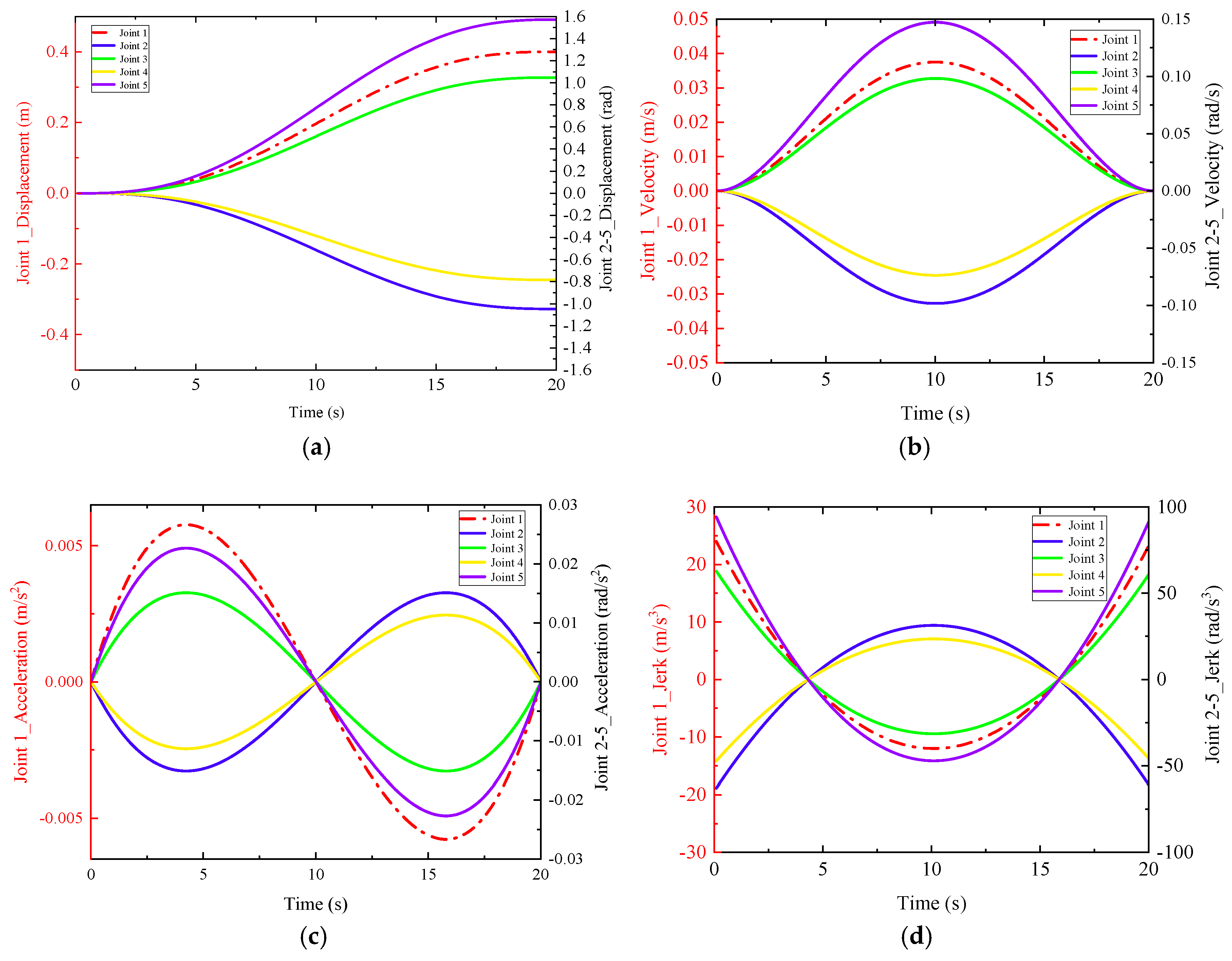
Joint space trajectory planning

Robot motion generally needs to be converted into a representation of joint space. When only the start and end time constraints are provided, this process is referred to as point-to-point path planning. During the planning, it is necessary to select a certain interpolation function in the joint space and select the optimal interpolation method according to the energy principle. There are many common interpolation functions, such as trapezoidal velocity interpolation [31], cubic polynomial interpolation [32], quintic polynomial interpolation [33], and so on. However, the velocity curve of the velocity trapezoid interpolation planning is not a smooth curve, which leads to the overshoot phenomenon caused by the acceleration mutation, and the cubic polynomial interpolation cannot constrain the acceleration of the beginning and end positions, which cannot plan a multi-segment continuous smooth trajectory. Therefore, quintic polynomial interpolation can solve the above problems caused by trapezoidal velocity interpolation and cubic polynomial interpolation because it can constrain the acceleration to ensure the continuity and smoothness of the trajectory. Thus, the joint value function $\theta \left(t\right)$, joint velocity function $\dot{\theta }\left(t\right)$, and joint acceleration function $\ddot{\theta }\left(t\right)$ changing with time $t$ are expressed as follows:

$$\begin{array}{c}\theta \left(t\right)=A_0+A_{1}t+A_2{t}^2+A_3{t}^3+A_4{t}^4+A_5{t}^5,\end{array}$$

(9)

$$\begin{array}{c}\dot{\theta }\left(t\right)=A_1+2A_{2}t+3A_3{t}^2+4A_4{t}^3+5A_5{t}^4,\end{array}$$

(10)

$$\begin{array}{c}\ddot{\theta }\left(t\right)=2A_2+6A_{3}t+12A_4{t}^2+20A_5{t}^3,\end{array}$$

(11)

where $A_i$ is the coefficient of time variable t of order $i$.

C.

Cartesian space trajectory planning

For conditions where the end effector must move along the planned trajectory, joint space trajectory planning with polynomial interpolation cannot achieve the desired planning effect. Thus, it is essential to plan the robot’s motion trajectory for completing welding tasks more accurately in Cartesian space. There are several common trajectory planning algorithms in Cartesian space, such as linear trajectory planning, circular trajectory planning, spline trajectory planning, and so on. The linear trajectory planning algorithm has the advantages of a simple algorithm, easy implementation, and good stability, and it can be used to verify the correctness of the urdf model.

We assume that the three-dimensional coordinates of the beginning and end points of the trajectory in Cartesian space are $P_0(X_0,Y_0,Z_0)$ and $P_1(X_1,Y_1,Z_1)$, respectively. The interpolation time interval is $\Delta t$ and the number of interpolations is $i$. The increments of adjacent interpolation points in each axis and the straight-line distance $L$ between the two points and are calculated as follows:

$$\begin{array}{c}\left\{\begin{array}{c}\Delta X={\displaystyle \frac{X_1-X_0}{N}}\\ \Delta Y={\displaystyle \frac{Y_1-Y_0}{N}}\\ \Delta Z={\displaystyle \frac{Z_1-Z_0}{N}}\end{array}\right.,\end{array}$$

(12)

$$\begin{array}{c}L=\sqrt{{\Delta X}^2+{\Delta Y}^2+{\Delta Z}^2}.\end{array}$$

(13)

Then, the total interpolation number is $N$. The interpolation distance $S_i$ of the time period $i·\Delta t$ and are calculated as follows:

$$\begin{array}{c}{S}_i={\displaystyle \frac{L}{N}}·i.\end{array}$$

(14)

Finally, the coordinates of the interpolation point $P_i$ are obtained as follows:

$$P_i=\left[\begin{array}{c}{X}_i\\ Y_i\\ Z_i\end{array}\right]=\left\{\begin{array}{c}{\displaystyle \frac{S_i}{L}}\times \Delta X+X_0\\ {\displaystyle \frac{S_i}{L}}\times \Delta Y+Y_0\\ {\displaystyle \frac{S_i}{L}}\times \Delta Z+Z_0\end{array}\right..$$

(15)

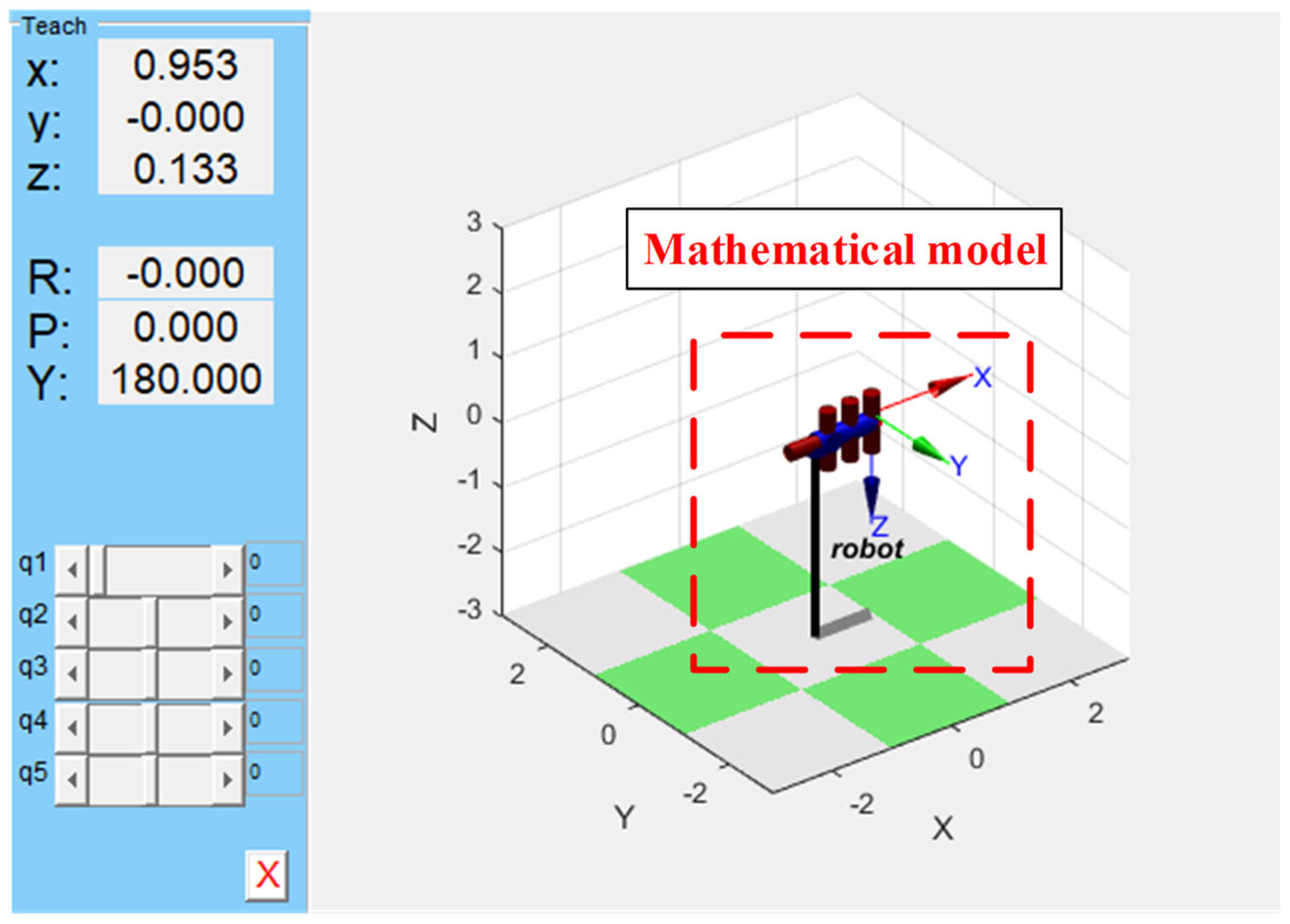
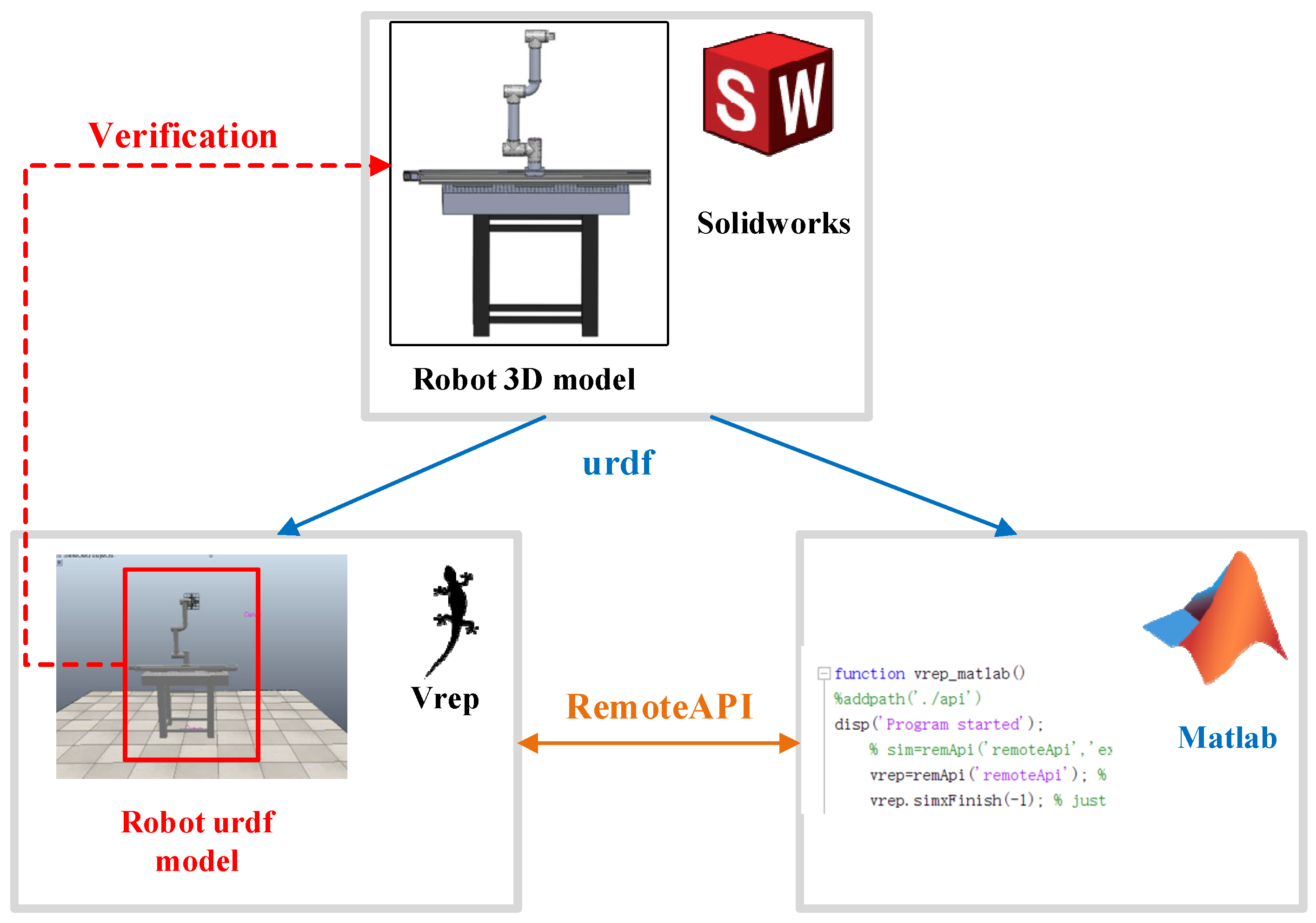
3.3. MBD: Robot Kinematics Simulation

The robot kinematics simulation, which includes the building of a co-simulation platform of Matlab 2018b and Vrep Edu and the simulation verification of trajectory planning, is a fast, low-cost, and effective method used to verify the correctness of the robot kinematics algorithm based on the robot 3D model and whether the robot of the MBD can complete the given task accurately and smoothly according to the planned trajectory, and it can further speed up the robot design process to shorten the development cycle and reduce costs.

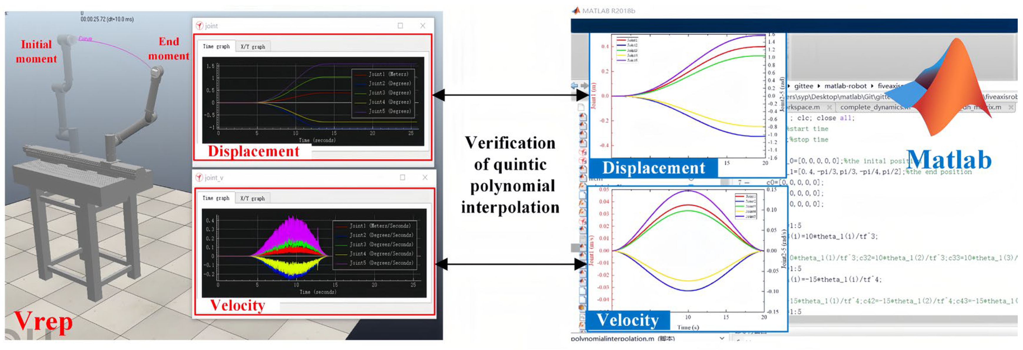
3.3.1. Co-Simulation Platform of Matlab 2018b and Vrep Edu

Vrep Edu (virtual robot experimentation platform) [34] is a software specially used for robot simulation. Its biggest advantage is that it can simulate synchronously or asynchronously with Matlab 2018b through scripts. The supported languages include C/C++, Python, Java, Lua, Matlab 2018b, and so on. A co-simulation platform of Matlab 2018b and Vrep Edu is built to test the linear trajectory planning algorithm. After designing the robot 3D model in Solidworks, it is imported into the Vrep Edu scene to generate the robot urdf model. RemoteAPI is used to communicate between Matlab 2018b and Vrep Edu to realize robot motion control. In addition, the reasonability of the robot urdf model can be verified by the physical engine of Vrep Edu, which provides a basis for the optimization of the robot 3D model. The robot simulation platform architecture is shown in Figure 9.

3.3.2. Simulation Verification of Trajectory Planning

The correctness of the trajectory planning algorithm can be verified using a co-simulation platform of Matlab 2018b and Vrep Edu, which includes the simulation verification of joint space trajectory planning and the simulation verification of Cartesian space trajectory planning. It demonstrates that the MBD robot can complete a given task accurately and smoothly according to the planned trajectory.

• Simulation verification of joint space trajectory planning

Firstly, according to the known conditions, including the joint value of the initial moment ${\theta }_0(\mathrm{0,0},\mathrm{0,0},0)$, the joint value of the end moment ${\theta }_f(0.4,-pi/3,pi/3,-pi/4,pi/2)$, initial joint velocity $v_0(=0 \mathrm{m}/\mathrm{s})$, end joint velocity $v_f(=0 \mathrm{m}/\mathrm{s})$, initial joint acceleration $a_0(=0 \mathrm{m}/{\mathrm{s}}^2)$, end joint acceleration $a_f(=0 \mathrm{m}/{\mathrm{s}}^2)$, starting time $t_0=0 \mathrm{s}$, and ending time $t_f=20 \mathrm{s}$, the coefficients $A_0$, $A_1$, $A_2$, $A_3$ can be solved as follows:

$$\begin{array}{c} A_0={\theta }_0{;A}_1=0{;A}_2=0{;A}_3={\displaystyle \frac{10}{{t_f}^3}}\left({\theta }_f-{\theta }_0\right){;A}_4={\displaystyle \frac{-15}{{t_f}^4}}\left({\theta }_f-{\theta }_0\right){;A}_5={\displaystyle \frac{6}{{t_f}^5}}\left({\theta }_f-{\theta }_0\right) .\end{array}$$

(16)

Then, a program using a quintic polynomial interpolation function to plan the robot joint space trajectory is written in Matlab 2018b. The plot function is used to plot the displacement, velocity, acceleration, and jerk curves of each joint during motion, as shown in Figure 10.

Finally, the displacement and velocity of each joint are sent to Vrep Edu in real time, which are recorded by a graph module.

It can be seen from Figure 11 that the displacement and velocity curve of each joint in Vrep Edu are the same as in Figure 10a,b, which verifies the correctness of the quintic polynomial interpolation algorithm and the urdf model and ensures the smoothness of the trajectory of the MBD robot in motion control.

B.

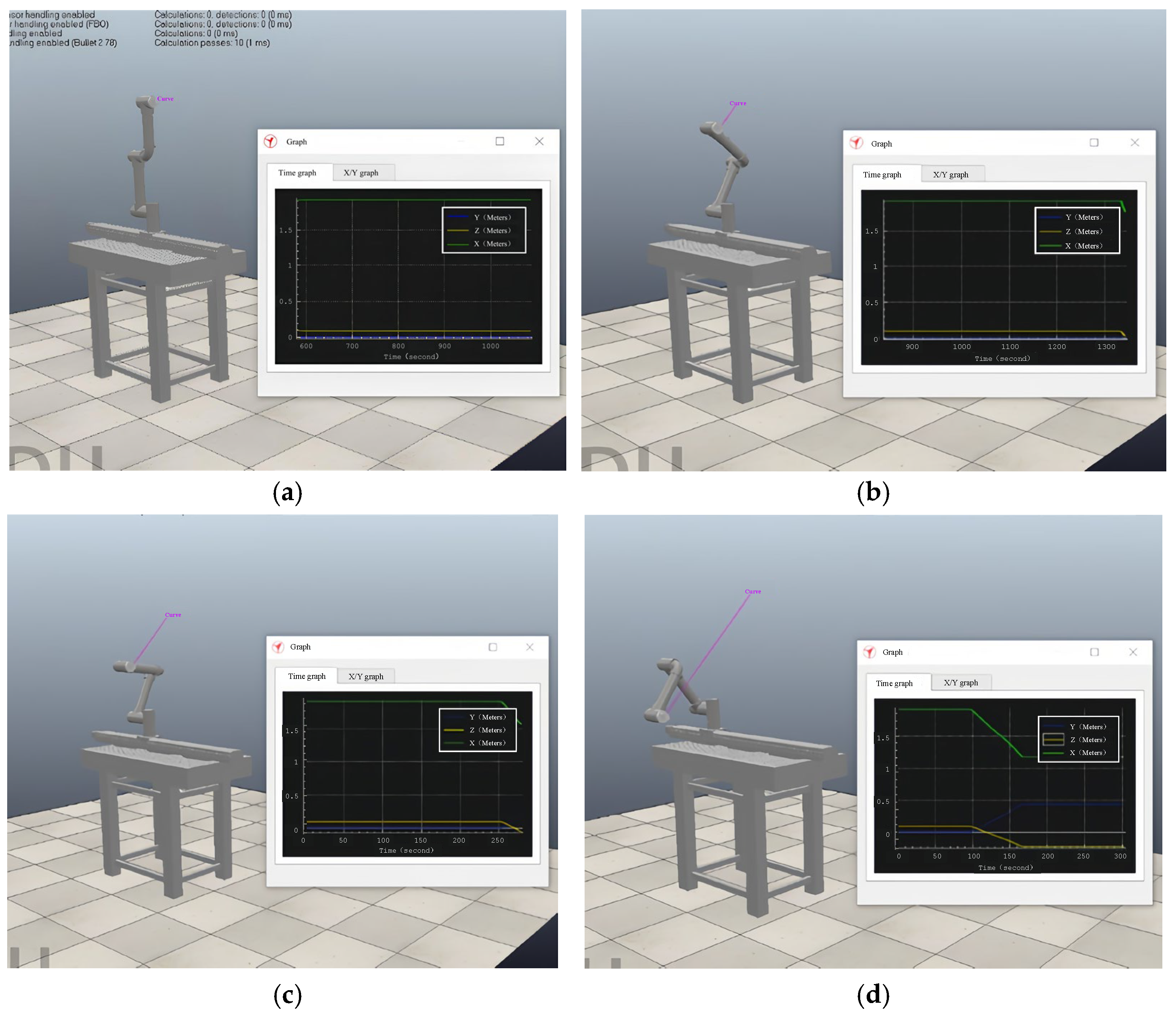
Simulation verification of Cartesian space trajectory planning

After setting the total interpolation number N to be 2000 and time T to be 20 s, according to Formula (15), the joint values of the robot corresponding to the interpolation point are obtained using a linear trajectory planning program written in Matlab 2018b and sent to Vrep Edu to control each joint move in real time. Thus, the real-time end effector position of the robot in Vrep Edu is shown in Figure 12. Since the coordinate system of joint 5 is shown in Figure 6 and the height h from the bottom of the slide table to the ground is 0.955 m, the real-time end effector position of the robot is as shown in Figure 12b, whose X is calculated by the X of Figure 12a, deducting the height h. Therefore, it can be seen from Figure 12 that the position curves of the end effector in the XYZ direction are the same as in Vrep Edu and are the same as the position curves in Matlab 2018b.

At the same time, the motion trajectory of the end effector at each moment is shown in Figure 13a–d, and its position is also recorded, using a graph module in Cartesian space.

It can be seen from Figure 13 that the motion trajectory is a straight line and the curve is continuous and smooth, which verifies the correctness of the linear trajectory planning algorithm. The completed joint space and Cartesian space trajectory planning simulation proves the ability of the MBD robot to complete a given task according to the planned trajectory and the correctness of the robot kinematics based on the 3D model.

4. Results and Discussion

After completing the rapid prototyping, robot kinematics, and robot kinematics simulation, the robot prototype is generated. Since there is a need to integrate it into the automatic welding production line, it is necessary to test the actual operational ability of the MBD robot prototype, which includes the development of the robot motion control system and the test of the MBD robot.

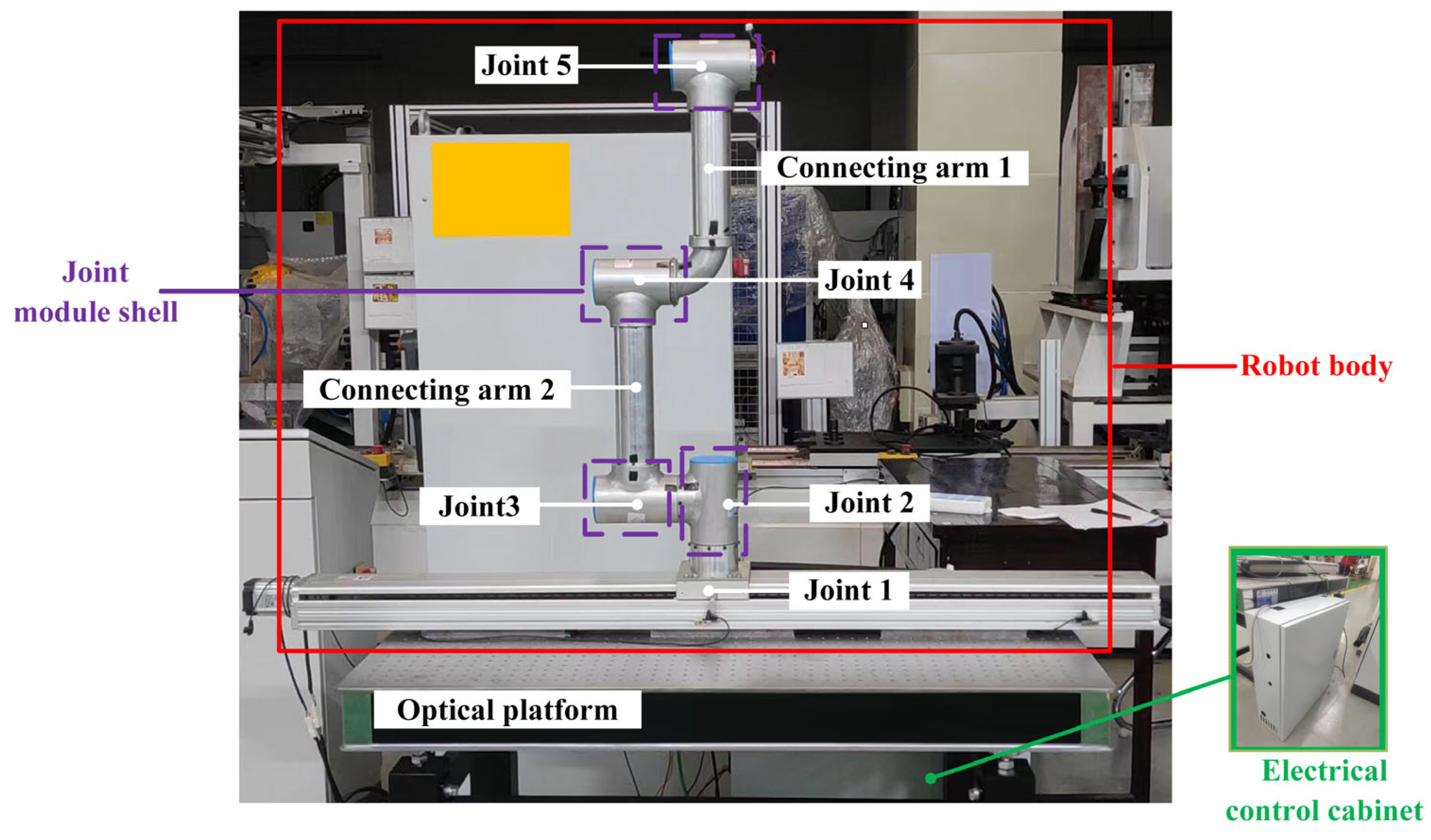
4.1. MBD: Robot Prototype

For lightweight purposes, the built robot prototype using MBD is shown in Figure 14, whose material of all connecting arms and joint module shells is made of aluminum alloy after completing the full optimization process of the robot 3D model. The robot body, composed of connecting arms and main components, is located on an optical platform and driven by the electrical control cabinet.

From the 3D model to the built prototype of the whole robot design process, the advantage of the MBD is that it can directly use the optimized three-dimensional model to complete the manufacturing quickly, reduce the possibility of secondary processing, and help quickly establish the MBD information node in the early stage of the design.

4.2. MBD: Robot Motion Control System and Test

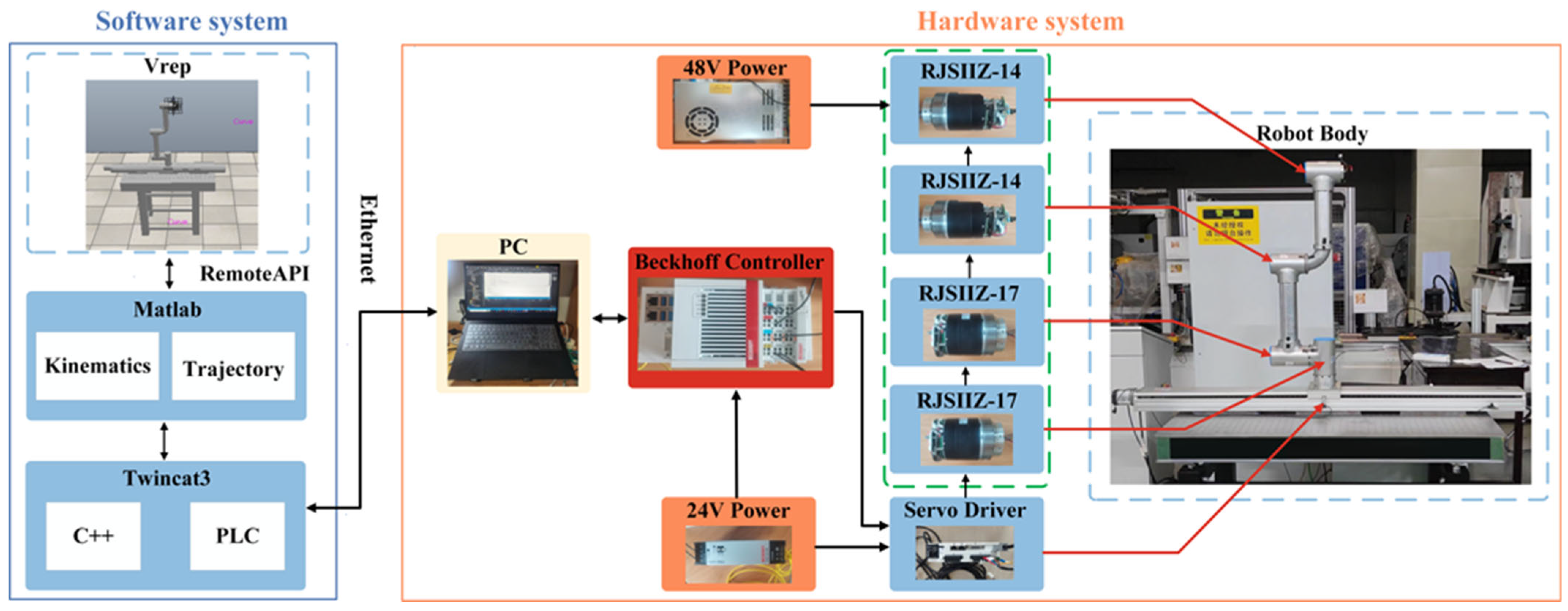
4.2.1. Robot Motion Control System

To realize the real control of the 5-DOFs light industrial MBD robot prototype, the robot motion control system is developed before testing the robot, which is shown in Figure 15. The robot motion control system consists of a software system and a hardware system. The software system includes Vrep Edu, Matlab 2018b, and Twincat3 software, which performs robot motion simulation and connects with the hardware system. The software system should complete kinematics and trajectory analysis by Matlab 2018b, robot motion simulation by the co-simulation platform of Matlab 2018b and Vrep Edu, C++ kinematics algorithm, and PLC control program writing by Twincat3 software [35], which develops motion control programs to generate motion control instructions. After the hardware system receives motion control instructions by Ethernet, the four joint modules and servo driver drive four revolute joints and the prismatic joint of the robot body, respectively, following the processed joint value signals by the Beckhoff controller through the EtherCAT protocol.

4.2.2. Robot Test

The test of the robot prototype quickly built by the 3D model is used to further verify the correctness of the trajectory planning algorithm in the actual operation of the motion control and the feasibility of designing a 5-DoFs light industrial robot based on MBD. It compares the prototype test results and the trajectory planning simulation results carried out by the model for consistency, and it includes the joint space trajectory planning experiment and the Cartesian space trajectory planning experiment.

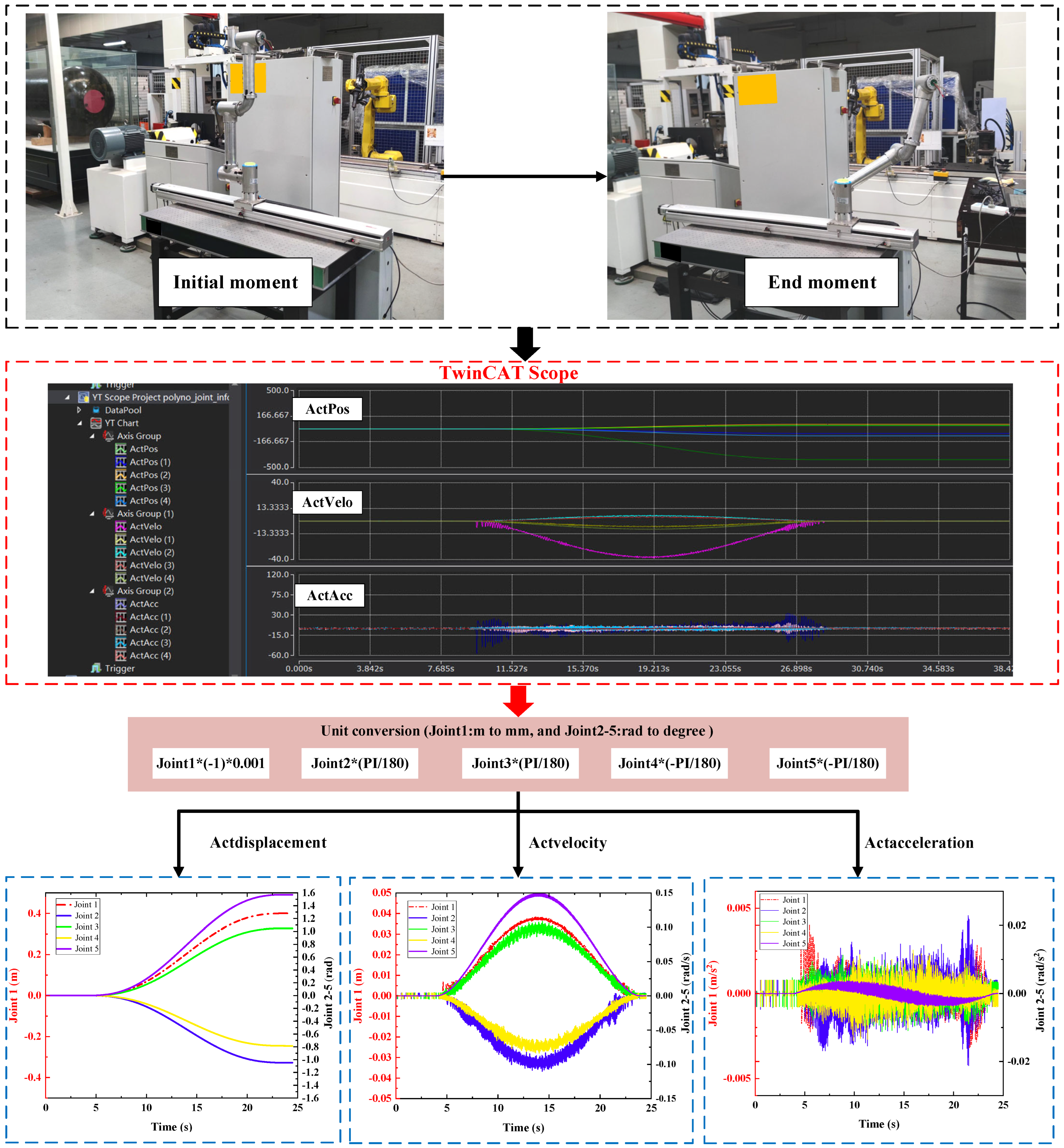
• Experiment with joint space trajectory planning

The correctness of the quintic polynomial interpolation algorithm (see Equations (9)–(11)) is tested by the designed robot motion control system. Figure 16 shows the joint position of the initial and end moment, which is recorded by the scope of Twincat in a total of 20 s. Thus, the curves of the actual displacement, velocity, and acceleration of each joint are generated through joint transformation.

B.

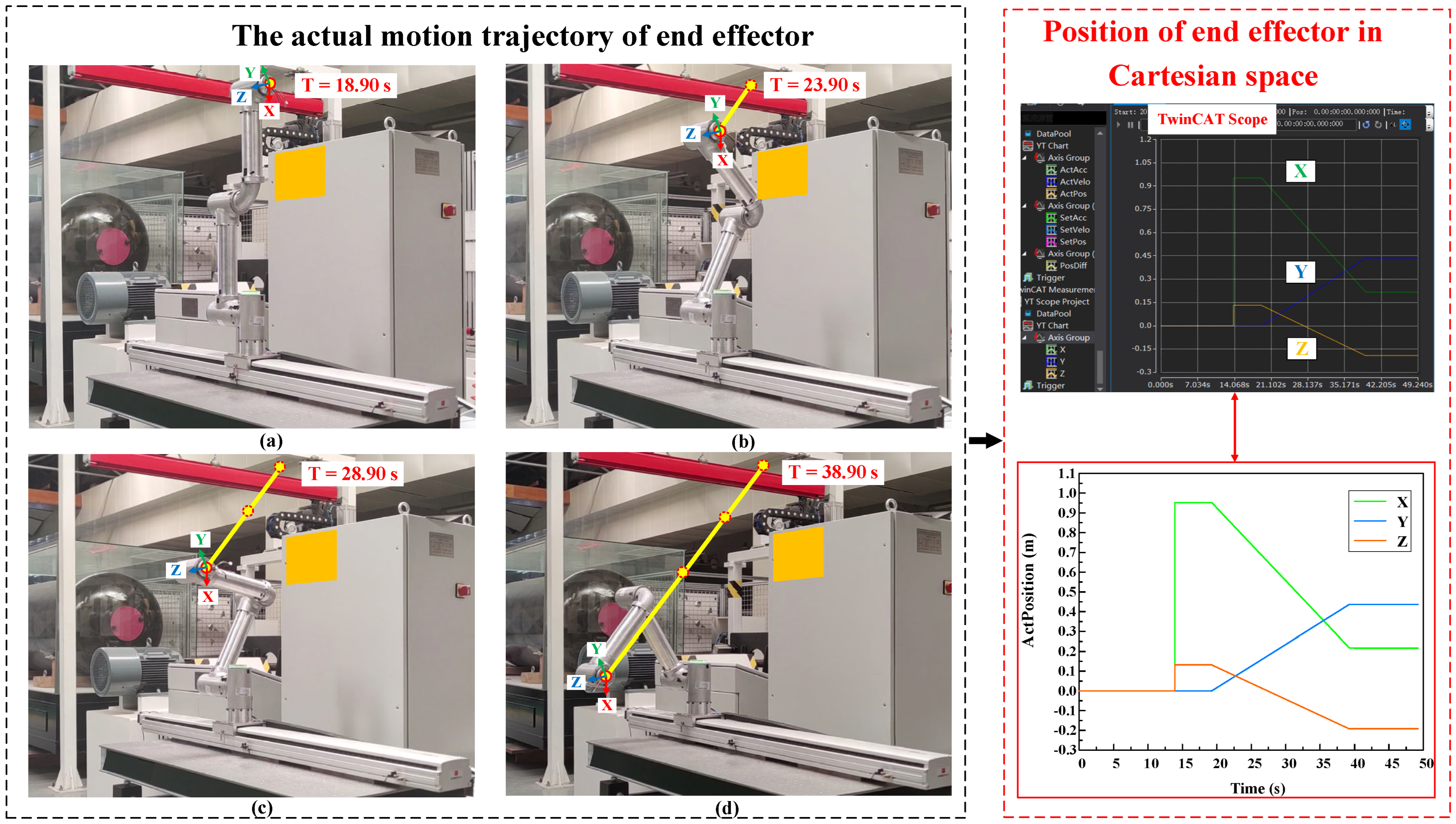
Experiment of Cartesian space trajectory planning

To guarantee that the robot can accurately track the planned trajectory, it is important to verify the correctness of the linear trajectory planning algorithm (see Equation (16)) in the Cartesian space through the above robot motion control system. Therefore, the motion trajectory of the end effector is carried out in the experiment and is shown in Figure 17.

It can be seen from Figure 17a–d that the actual motion trajectory of the end effector is a straight line from the initial moment 18.09 s to the end moment 38.90 s and the actual position of the end effector in the Cartesian space is recorded by TwinCAT scope, which not only proves the correctness of the linear trajectory algorithm but also verifies the feasibility of MBD by combining the experiment of joint space trajectory planning. The experimental video is available online (https://github.com/sypaaaaa/The-straight-line-motion-trajectory.git accessed on 10 September 2024).

5. Conclusions

In this paper, the MBD method of a 5-DoF light industrial robot is proposed. The robot’s 3D model is generated by completing the robot design preparation according to the robot design requirements. The robot design can be finished using several design methods, such as rapid prototyping, robot kinematics, and robot kinematics simulation. The joint component verification and selection of the robot are used to further optimize the robot’s 3D model by the robot’s Adams kinematics model for rapid prototyping. To realize the motion control of the MBD robot according to robotics, the robot kinematics algorithm provides a theoretical basis for the robot’s 3D model design and proves the reasonability of the motion control of the robot by the generated mathematical model, including kinematics analysis and trajectory planning. The robot kinematics simulation verifies whether the robot can complete a given task according to the planned trajectory, and the correctness of the robot kinematics algorithm is verified by the robot urdf model. Finally, the correctness of the trajectory algorithm and the feasibility of MBD have been verified by the generation output of the robot prototype and the test of the developed motion control system. This MBD of a 5-DOF light industrial robot in this paper is a general method of robot design, which helps complete the process of the robot prototype design quickly and effectively to shorten the prototype design cycle and reduce the cost of secondary selection design, as well as accelerate the development of the robot motion control system. However, some specific automation conditions cannot be satisfied by the trajectory planning of the robot.

Future work will focus on integrating robot dynamics into the MBD framework to enable optimal trajectory planning under dynamic constraints and support real-time adaptive control, thereby improving motion performance and system robustness. There is also a plan to implement MBD in more complex industrial robots with larger DoF to verify the feasibility of the approach. Although the proposed MBD approach demonstrates high efficiency, it may not directly apply to systems with dynamic uncertainties or environments requiring high payloads.

References

1. Alghazzawi, T.F. Advancements in CAD/CAM technology: Options for practical implementation. J. Prosthodont. Res. 2016, 60, 72–84. [Google Scholar] [CrossRef] [PubMed]
2. Della Bona, A.; Nogueira, A.D.; Pecho, O.E. Optical properties of CAD–CAM ceramic systems. J. Dent. 2014, 42, 1202–1209. [Google Scholar] [CrossRef] [PubMed]
3. Derby, S. Workcell Based Robot Design Methodologies. In Proceedings of the International Design Engineering Technical Conferences and Computers and Information in Engineering Conference, American Society of Mechanical Engineers, Atlanta, GA, USA, 13–16 September 1998; p. USAV01BT01A016. [Google Scholar]
4. Wen, L.G.; Wu, H.T.; Liu, H.B. The Design of Mechanical Arm of Hot Extruding and Upsetting Machine Based on SolidWorks. Adv. Mater. Res. 2013, 655–657, 269–272. [Google Scholar] [CrossRef]
5. Mekhnacha, K.; Mazer, E.; Bessière, P. The design and implementation of a Bayesian CAD modeler for robotic applications. Adv. Robot. 2001, 15, 45–69. [Google Scholar] [CrossRef]
6. Liu, Q.; Yang, D.; Hao, W.; Wei, Y. Research on kinematic modeling and analysis methods of UR robot. In Proceedings of the 2018 IEEE 4th Information Technology and Mechatronics Engineering Conference (ITOEC), Chongqing, China, 14–16 December 2018; IEEE: Piscataway, NJ, USA, 2018; pp. 159–164. [Google Scholar]
7. Ponsà Cobas, S. Strategies for Remote Control and Teleoperation of a UR Robot; Universitat Politècnica de Catalunya: Barcelona, Spain, 2020. [Google Scholar]
8. Zafra Navarro, A.; Guillén Pastor, J. UR Robot Scripting and Offline Programming in a Virtual Reality Environment; Universidad de Alicante: Alicante, Spain, 2021. [Google Scholar]
9. Arbo, M.; Eriksen, I.; Sanfilippo, F.; Gravdahl, J. Comparison of KVP and RSI for controlling KUKA robots over ROS. IFAC-PapersOnLine 2020, 53, 9841–9846. [Google Scholar] [CrossRef]
10. Schreiber, G.; Stemmer, A.; Bischoff, R. The fast research interface for the kuka lightweight robot. In Proceedings of the IEEE Workshop on Innovative Robot Control Architectures for Demanding (Research) Applications How to Modify and Enhance Commercial Controllers (ICRA 2010), Anchorage, Alaska, 3 May 2010; pp. 15–21. [Google Scholar]
11. Shepherd, S.; Buchstab, A. Kuka robots on-site. In Robotic Fabrication in Architecture, Art and Design 2014; Springer: Berlin/Heidelberg, Germany, 2014; pp. 373–380. [Google Scholar]
12. Gao, X.; Jiang, H.; Zhang, H. Research and Application of Spacecraft Pipeline Digital Development Mode Based on MBD Technology. J. Phys. Conf. Ser. 2021, 1865, 032028. [Google Scholar] [CrossRef]
13. Zhu, H.; Li, J. Research on three-dimensional digital process planning based on MBD. Kybernetes 2018, 47, 816–830. [Google Scholar] [CrossRef]
14. Mahapatra, S. Using model-based design for hybrid electric vehicle systems. Electron. Wkly. 2010, 2416. [Google Scholar]
15. Steinbauer, T.; Leiprecht, G.; Havraneck, W. High performance HIL real time for the Airbus A380 electrical backup hydraulic actuators. In Proceedings of the UKACC Control 2004 Mini Symposia, Bath, UK, 8 September 2004. [Google Scholar]
16. Yim, M.; Shen, W.M.; Salemi, B.; Rus, D.; Moll, M.; Lipson, H.; Klavins, E.; Chirikjian, G.S. Modular self-reconfigurable robot systems [grand challenges of robotics. IEEE Robot. Autom. Mag. 2007, 14, 43–52. [Google Scholar] [CrossRef]
17. Mamani-Saico, A.; Yanyachi, P.R. Implementation and performance study of the micro-ros/ros2 framework to algorithm design for attitude determination and control system. IEEE Access 2023, 11, 128451–128460. [Google Scholar] [CrossRef]
18. Franklin, C.S.; Dominguez, E.G.; Fryman, J.D.; Lewandowski, M.L. Collaborative robotics: New era of human–robot cooperation in the workplace. J. Saf. Res. 2020, 74, 153–160. [Google Scholar] [CrossRef] [PubMed]
19. Lo, A.K.-Y.; Yang, Y.-H.; Lin, T.-C.; Chu, C.-W.; Lin, P.-C. Model-based design and evaluation of a brachiating monkey robot with an active waist. Appl. Sci. 2017, 7, 947. [Google Scholar] [CrossRef]
20. Daniel Alamsyah, M.I.; Erwin Tan, S. Serpentine Robot Model and Gait Design Using Autodesk Inventor and Simulink SimMechanics. EPJ Web Conf. 2014, 68, 1–4. [Google Scholar] [CrossRef]
21. Wang, R.; Song, Y.; Dai, J.S. Reconfigurability of the origami-inspired in-tegrated 8R kinematotropic metamorphic mechanism and its evolved 6R and 4R mechanisms. Mech. Mach. Theory 2021, 161, 104245. [Google Scholar] [CrossRef]
22. Sabnis, C.; Anjana, N.; Talli, A.; Giriyapur, A.C. Modelling and simulation of industrial robot using SolidWorks. In Advances in Industrial Machines and Mechanisms: Select, Proceedings of the IPROMM 2020, Telangana, India, 21–22 December 2020; Springer: Berlin/Heidelberg, Germany, 2020; pp. 173–182. [Google Scholar]
23. Cheraghpour, F.; Vaezi, M.; Jazeh, H.E.S.; Moosavian, S.A.A. Dynamic modeling and kinematic simulation of Stäubli© TX40 robot using MATLAB/ADAMS co-simulation. In Proceedings of the 2011 IEEE International Conference on Mechatronics, Istanbul, Turkey, 13–15 April 2011; pp. 386–391. [Google Scholar]
24. Wang, Z.; Liu, Y.; Liu, L. Research on SDH Model Calibration Algorithm for Robotic Arm Based on Differential Transform. Math. Probl. Eng. 2022, 2022, 1–9. [Google Scholar] [CrossRef]
25. Deng, X.; Ge, L.; Li, R.; Liu, Z. Research on the kinematic parameter calibration method of industrial robot based on LM and PF algorithm. In Proceedings of the 2020 Chinese Control And Decision Conference (CCDC), Hefei, China, 22–24 August 2020; pp. 2198–2203. [Google Scholar]
26. Jia, G.; Li, B.; Dai, J.S. Oriblock: The origami-blocks based on hinged dissection. Mech. Mach. Theory 2024, 203, 105826. [Google Scholar] [CrossRef]
27. Liu, H.; Yan, Z.; Xiao, J. Pose error prediction and real-time compensation of a 5-DOF hybrid robot. Mech. Mach. Theory 2022, 170, 104737. [Google Scholar] [CrossRef]
28. Peng, W.; Yiren, Z.; Nan, Y. An Inverse Solution Algorithm for Industrial Robot. J. Phys. Conf. Ser. 2022, 2173, 469. [Google Scholar]
29. Janson, L.; Schmerling, E.; Pavone, M. Monte Carlo motion planning for robot trajectory optimization under uncertainty. In Robotics Research; Springer: Berlin/Heidelberg, Germany, 2017; Volume 2, pp. 343–361. [Google Scholar]
30. Long, D.T.; Binh, T.; Hoa, R.; Anh, L.; Toan, N. Robotic arm simulation by using matlab and robotics toolbox for industry application. Int. J. Electron. Commun. Eng. 2020, 7, 1–4. [Google Scholar] [CrossRef]
31. Heo, H.-J.; Son, Y.; Kim, J.-M. A Trapezoidal Velocity Profile Generator for Position Control Using a Feedback Strategy. Energies 2019, 12, 1222. [Google Scholar] [CrossRef]
32. Cai, Z. Cubic Polynomial Smooth Support Vector Machine Used in Intrusion Detection. In Proceedings of the 2016 3rd International Conference on Materials Engineering, Manufacturing Technology and Control, Taiyuan, China, 27–28 February 2016; pp. 1236–1239. [Google Scholar]
33. Lu, S.; Ding, B.; Li, Y. Minimum-jerk trajectory planning pertaining to a translational 3-degree-of-freedom parallel manipulator through piecewise quintic polynomials interpolation. Adv. Mech. Eng. 2020, 12, 1687814020913667. [Google Scholar] [CrossRef]
34. Fontanelli, G.A.; Selvaggio, M.; Ferro, M.; Ficuciello, F.; Vendittelli, M.; Siciliano, B. A v-rep simulator for the da vinci research kit robotic platform. In Proceedings of the 2018 7th IEEE International Conference on Biomedical Robotics and Biomechatronics (Biorob), Enschede, The Netherlands, 26–29 August 2018; pp. 1056–1061. [Google Scholar]
35. Lovrec, D.; Tič, V.J.I. Comparison of different position controllers implemented with a Beckhoff controller and TwinCAT 3 software. Elektron. Viri 2022, 10, 83–86. [Google Scholar]
Figure 1. MBD: The design flow chart of the robot.
Robotics 14 00103 g001
Figure 2. MBD: The robot structure.
Robotics 14 00103 g002
Figure 3. MBD: The robot 3D model.
Robotics 14 00103 g003
Figure 4. MBD: The robot Adams kinematics model, where joint 1 is the prismatic joint, and joints 2–5 are revolute joints.
Robotics 14 00103 g004
Figure 5. MBD: A joint force/torque curve after verification.
Robotics 14 00103 g005
Figure 6. MBD: The robot coordinate system established by SD-H.
Robotics 14 00103 g006
Figure 7. MBD: The robot mathematical model in Matlab 2018b.
Robotics 14 00103 g007
Figure 8. MBD: The robot workspace cloud map: (a) 3D view; (b) x o z planar projection; (c) y o z planar projection; (d) x o y planar projection.
Robotics 14 00103 g008
Figure 9. MBD: The robot simulation platform architecture.
Robotics 14 00103 g009
Figure 10. MBD: The information of each joint in Matlab 2018b: (a) displacement; (b) velocity; (c) acceleration; (d) jerk.
Robotics 14 00103 g010
Figure 11. MBD: Real-time joint information in Vrep Edu.
Robotics 14 00103 g011
Figure 12. MBD: The real-time end effector position: (a) Vrep Edu; (b) Matlab 2018b.
Robotics 14 00103 g012
Figure 13. MBD: The motion trajectory of the end effector in Vrep Edu: (a) T = 0 s initial moment; (b) T = 5 s middle time; (c) T = 10 s middle time; (d) T = 20 s middle time.
Robotics 14 00103 g013
Figure 14. MBD: The robot prototype.
Robotics 14 00103 g014
Figure 15. MBD: The robot motion control system.
Robotics 14 00103 g015
Figure 16. MBD: The actual information of each joint in Twincat3.
Robotics 14 00103 g016
Figure 17. MBD: The actual motion trajectory of the end effector: (a) T = 18.90 s initial moment; (b) T = 23.90 s middle moment; (c) T = 28.90 s middle moment; (d) T = 38.90 s end moment.
Robotics 14 00103 g017