Methodology for Modeling Coupled Rigid Multibody Systems Using Unitary Quaternions: The Case of Planar RRR and Spatial PRRS Parallel Robots

Abstract

Quaternions are used in various applications, especially in those where it is necessary to model and represent rotational movements, both in the plane and in space, such as in the modeling of the movements of robots and mechanisms. In this article, a methodology to model the rigid rotations of coupled bodies by means of unit quaternions is presented. Two parallel robots were modeled: a planar RRR robot and a spatial motion PRRS robot using the proposed methodology. Inverse kinematic problems were formulated for both models. The planar RRR robot model generated a system of 21 nonlinear equations and 18 unknowns and a system of 36 nonlinear equations and 33 unknowns for the case of space robot PRRS; both systems of equations were of the polynomial algebraic type. The systems of equations were solved using the Broyden–Fletcher–Goldfarb–Shanno nonlinear programming algorithm and Mathematica V12 symbolic computation software. The modeling methodology and the algebra of unitary quaternions allowed the systematic study of the movements of both robots and the generation of mathematical models clearly and functionally.

1. Introduction

The kinematic and dynamic study of parallel robots is difficult and complicated since they are made up of several loops and closed kinematic chains [1]. There are important differences between serial and parallel configuration robots, for example, due to the latter’s robust structure, higher load capacity, versatility, and excellent positioning accuracy [2].

In fact, in industrial automation, parallel manipulators have been considered an alternative to traditional automation to achieve a high load capacity and precise positioning for higher quality and more economical processes [3]. The main disadvantages of parallel robots are their small workspace and the singularities that can appear within them [2].

Parallel robots are currently used in various applications, such as machining operations [4], additive manufacturing for construction [5], and dimensional metrology [6]. This type of robot is also used for medical operations [7] and in rehabilitation [8], as well as in flight simulators [9] and in telescope mechanisms [10], among others.

For the kinematic modeling of parallel robots, there are several mathematical methods and tools. Homogeneous matrices and Denavit–Hartenberg parameters [D-H] are regularly used for the kinematic modeling of this type of robot [11,12]. Also, geometrical methods have been used to study the planar motion of parallel-type robots [13,14] and their singularities [15]. Screw theory is also used in the modeling of parallel robots [16,17]. Complex number algebra [18] and quaternions [19,20] are used to model robot rotations in the plane and in space, respectively. Other versions of quaternions, such as dual representations, are also applied to the modeling of parallel robots [21,22].

While each mathematical tool and modeling method used to study parallel robots has its advantages and disadvantages, quaternions stand out due to their compact notation and ease of composition, and they are more efficient than matrix methods, involving fewer algebraic operations and, hence, less computational storage. In fact, the performance of dual quaternions has been shown to improve by 30–40% in forward kinematics over conventional homogeneous transformation matrices [23]. These and other important features of quaternions and their representations make them ideal for modeling parallel robots. Recently, a PUMA robot has been modeled with the algebra of quaternions [24]. In this work, the systematization of the quaternions developed in 1990 at INRIA France [25,26] was applied. The results showed that it was possible to model the rotations of the links of an open chain robot clearly and systematically, performing all the operations in the vector space of quaternions and avoiding the use of trigonometric relations during modeling. The PUMA robot was modeled using sequences of rotations, and the numerical solution of the mathematical model associated with the inverse kinematics was obtained with the Newton–Raphson method.

In other works, quaternions have been applied to the analysis and synthesis of parallel robots; for example, in [27], the kinematic synthesis problem of a planar parallel robot of RPR configuration was modeled using Quaternions. The generated model allowed for achieving any desired configuration, and the definition of the problem in the space of planar quaternions resulted in a definition of the workspace of the parallel manipulator as the intersection of quadratic equations. In another study, the modes of operation and transition configurations of the parallel cylindrical mechanism 1-RPU-2-UPU were analyzed [28]. In that study, a reconfiguration analysis of a parallel manipulator was performed, and the constraint equations were modeled using the Euler parameter quaternion. Liu et al. [29] proposed an analytical algorithm using unitary quaternions to model the direct kinematics of a 6-UPS parallel robot with an additional displacement sensor mounted at the top and bottom platform centers. Birlescu et al. [30] proposed a mathematical method to redefine motion parameterizations based on the joint space representation of parallel robots. The mathematical models were developed using dual quaternions, and the main feature of the model was that, instead of directly studying the motion of the moving platform, the joint space of the mechanism was analyzed by eliminating the study parameters. Finally, Dong et al. [31] analyzed the motions of a 6RUS parallel manipulator using dual quaternions.

On the other hand, many mathematical models related to robot motions and mechanisms consider the unitary norm of quaternions, which implies that the systems of equations are nonlinear. To solve this type of problem, the Newton–Raphson method is commonly used [24]. Quasi-Newton methods and the Davidon–Fletcher–Powell (DFP) algorithm have also been used to solve mathematical models of robots and mechanisms. For example, in [32], the DFP algorithm was applied to determine the numerical solution and optimization of some dependent motions accompanying some independent motions called “parasitic motions” of a 3 DOF parallel robot. There are several variants of the quasi-Newton methods, and in all of them, the idea is to consider the Hessian matrix in the quadratic model. The Broyden–Fletcher–Goldfarb–Shanno (BFGS) method is a variant of the DFP method and was used by Kashyap and Parhi (Kumar; Dayal) [33] to solve a path planning problem for a humanoid robot. In turn, Xie et al. [34] used the BFGS algorithm, the Newton–Raphson method, and the Levenberg–Marquardt algorithm to compute the inverse kinematic problem for a 7 DOF open-chain robot.

On the other hand, the spatial PRRS configuration robot and the RRR parallel robot stand out among the existing set of spatial robots and parallel planes. The PRRS space robot has been studied in [35], where its design was developed using structural synthesis modeling and degrees of freedom analysis. On the other hand, the RRR planar robot, due to its simple configuration, has been used to test different kinematic and dynamic modeling [36,37]. In other works, this robot was used to develop artificial intelligence tests [38,39] and to test different control models [40,41], as well as for the study and analysis of singularities [42,43].

This paper describes and applies a novel methodology using unitary quaternions to study parallel robot motions of PRRS and RRR configurations, respectively. This methodological proposal is a continuation of the modeling method described in [24] and aims to extend the applications of the quaternion systematization developed by Reyes [25,26] to other types of robots, in this case, to the study of parallel robots. With the mathematical models generated for each robot analyzed, inverse kinematic problems were formulated. These problems were solved using the formal calculation platform Mathematica V12. The novelties of this work with respect to the results presented in [24] are as follows: (1) for the modeling of the robots under study, two configurations are not considered, (2) the mathematical models generated are nonsquare and nonlinear, and (3) the solution method used was the BFGS optimization method [44,45,46]. Although there are already several methodologies that take quaternions into account as the basis for modeling robot motions [24,47,48,49,50,51,52], the method proposed in this paper is general and can be applied to model parallel robots in the plane and in space.

2. Materials and Methods

In this section, a summary of the theoretical framework of Quaternion algebra and the methodology to systematize rotations using unitary quaternions is presented. In addition, modeling of RRR and PRRS robots of parallel configuration is developed. The inverse kinematic problems for both robots are formulated, and the BFGS optimization method with which the generated mathematical models were solved is described.

2.1. Preliminaries of the Algebra of Quaternions

A systematic way of constructing the algebra of quaternions with a modern linear algebra focus is presented in [24,25,26]. Let the set ℜ⁴, on which the binary operations are defined ⊕: ℜ⁴ × ℜ⁴→ℜ⁴, and ∗: ℜ⁴ × ℜ⁴→ℜ⁴ be expressed:

(i) (a,b,c,d) ⊕ (α,β,γ,δ) = (a + α, b + β, c + γ, d + δ)

(1)

(ii) (a,b,c,d) ∗ (α,β,γ,δ) = (aα − bβ − cγ − dδ, aβ + bα + cδ − dγ, aγ − bδ + cα + dβ,
aδ + bγ − cβ + dα ), ∀ (a,b,c,d), (α,β,γ,δ) ∈ ℜ^4.

The pairs (ℜ⁴,⊕) and (ℜ⁴,∗) form a commutative additive group and a non-commutative multiplicative group, respectively. The triple (ℜ⁴,⊕,∗) forms a non-commutative field. This is as follows:

(i)

The operation ∗:ℜ⁴×ℜ⁴→ℜ⁴ is associative, since

p∗(q∗s) = (p∗q)∗s; ∀ p, q, s∈ℜ⁴.

(2)

(ii)

The element 1 = (1,0,0,0) ∈ ℜ⁴ is such that: 1∗p = p∗1 = p, ∀p∈ℜ⁴. This element is known as the neutral element of the multiplication in ℜ⁴.

(iii)

∀p∈ℜ⁴, p ≠ (0,0,0,0); p′∈ℜ⁴ such that p∗p′ = 1. The element p′ is called the multiplicative inverse of the quaternion p.

(iv)

The operation ∗:ℜ⁴ × ℜ⁴→ℜ⁴ is not commutative. This is p∗q ≠ q∗p.

(v)

The following distributive properties are satisfied:

(a) (p⊕q)∗s = p∗s ⊕ q∗s
       (b) p∗(q⊕s) = p∗q ⊕ p∗s, ∀p, q, s∈ℜ⁴

(3)

On the other hand, the operation •: ℜ × ℜ⁴→ℜ⁴ is defined by the following:

α•(a,b,c,d)= (αa,αb,αc,αd),  ∀(a,b,c,d)∈ℜ⁴, α∈ℜ

(4)

It is a scalar product on ℜ⁴, so the term (ℜ⁴, ⊕, •) is a real vector space. The transformation <•,•>:ℜ⁴ × ℜ⁴→ℜ, is defined by the following:

$$<\mathbf{p},\mathbf{q}>={\sum }_{\mathrm{i}=0}^3{\mathrm{p}}_{\mathrm{i}}{\mathrm{q}}_{\mathrm{i}}\in \Re$$

(5)

It is an inner product in ℜ⁴ and, therefore, the structure Q = (ℜ⁴, ⊕, ∗, •, <•, •>) is a real vector space with inner product, and the norm associated with this inner product is the following:

‖p‖ = <p,p>^1/2 = (p₀² + p₁² + p₂² + p₃²)^1/2

(6)

For which the structure Q = (ℜ⁴,⊕,∗,•, |•|) is a normed space, which will be called the vector space of quaternions, and its elements will be called quaternions [25].

It is possible to represent a quaternion as the sum of a real quaternion and a vector quaternion. Let the following subsets be as follows:

Q_r = {(a,0,0,0): a∈ℜ}⊂Q,
 Q_v = {(0,b,c,d): b,c,d∈ℜ}⊂Q

(7)

The transformations are defined by the following:

T_r(a,0,0,0) = a    ∀(a,0,0,0)∈Q_r
T_v(0,b,c,d) = (b,c,d)  ∀(0,b,c,d)∈Q_v

(8)

are isomorphic, and, therefore, if p = (a,b,c,d)∈Q, then

$$\mathbf{p} ={\mathbf{T}}_{\mathbf{r}}^{-1}\left(\mathrm{a}\right) \oplus {\mathbf{T}}_{\mathbf{v}}^{-1}(\mathrm{b}, \mathrm{c}, \mathrm{d})$$

(9)

In a similar way to the algebra of complex numbers, a conjugate quaternion can be defined as follows:

$$\stackrel{\_}{\mathbf{p}}=\left(\mathrm{a},-\mathrm{b},-\mathrm{c},-\mathrm{d}\right)$$

(10)

given p = (p₀, p₁, p₂, p₃) and q = (q₀, q₁, q₂, q₃) ∈Q, then

$$(1) \stackrel{\_}{\mathbf{p}\oplus \mathbf{q}}=\stackrel{\mathrm{\_}}{\mathbf{p}}\oplus \stackrel{\mathrm{\_}}{\mathbf{q}}$$

(11)

$$(2) \stackrel{\mathrm{\_}}{\mathbf{p}\ast \mathbf{q}}=\stackrel{\mathrm{\_}}{\mathbf{q}}\ast \stackrel{\mathrm{\_}}{\mathbf{p}}$$

$$(3) \mathbf{p}\ast \stackrel{\mathrm{\_}}{\mathbf{p}}=\stackrel{\mathrm{\_}}{\mathbf{p}}\ast \mathbf{p}\in {\mathbf{Q}}_{\mathbf{r}}$$

2.2. Parametric Representation of Rotations of a Rigid Body

Let ρ(p,•):Q→Q, p∈Q be a linear transformation defined by the following:

$$\rho \left(\mathbf{p},\mathbf{q}\right)=\mathbf{p}\ast \mathbf{q}\ast {\mathbf{p}}^{-1}={\displaystyle \frac{1}{{‖\mathbf{p}‖}^2}}•\left(\mathbf{p}\ast \mathbf{q}\ast \stackrel{\mathrm{\_}}{\mathbf{p}}\right),\forall \mathbf{p},\mathbf{q}\in \mathbf{Q}$$

(12)

This function is a rotation that preserves the inner product, the norm, and the angle [25]. The transformation ρ(p,•):Q→Q, is linear, orthogonal, and ρ(p, q)∈Q_v, by all q∈Q_v. Let θ∈[0, nπ], n∈ℵ, w∈Q_v, ‖w‖ = 1; then, the quaternion p∈Q, with p₀∈ℜ−{0} and p_v = ±sinθw, is such that ρ(p, w) = w, where p₀ satisfies the equation

4 p₀⁴ − 4 p₀² ‖p‖²cosθ − ‖p‖⁴sin²θ = 0

(13)

The quaternion p represents a rotation of angle θ∈[0, nπ], with axis w∈Q_v, giving the following:

p₀ = ‖p‖ cos(θ/2), p_v = ±‖p‖sin(θ/2)w

(14)

In general, the norm of p can be arbitrary. Unit quaternions will be used in this article; that is, ‖p‖ = 1, so expression (14) reduces to the following:

p₀ = cos(θ/2), p_v = ±sin(θ/2)w

(15)

2.3. Kinematic Modeling of Coupled Bodies

In this section, a methodology based on quaternion algebra is presented and applied to model the rotations of kinematic chains associated with robots and mechanisms. This methodology will be applied to subsequently model the robots of RRR and PRRS configurations studied in this work. The modeling process involves a representation of a rigid body to determine the position of a point on it with respect to an inertial reference system. To achieve a systematic representation of the rotations, it is necessary to define functions that allow transforming vectors defined in ℜ³ to the Q space and vice versa.

2.3.1. Isomorphism of the Vectors of ℜ³ to the Vector Space Q

It is possible to define a function T_v: Q_v→ℜ³, between the subspace of the vector quaternion Q_v and the vector space ℜ³, according to expressions (8). This is as follows:

T_v(0,b,c,d) = (b,c,d); ∀(0,b,c,d) ∈Q_v

Subsequently, the transformations described by expressions (8) are isomorphic; then, there is an inverse transformation ${\mathbf{T}}_{\mathbf{v}}^{-1}$: ℜ³→Q_v, such that

$${\mathbf{T}}_{\mathbf{v}}^{-1}(\mathrm{b},\mathrm{c},\mathrm{d})=(0,\mathrm{b},\mathrm{c},\mathrm{d}); \forall (\mathrm{b},\mathrm{c},\mathrm{d})\in {\Re }^3$$

(16)

Therefore, any vector of ℜ³ can be considered an element of the vector space of quaternions [25]. Thus, by applying the proposed isomorphism of expression (16) to the canonical basis in ℜ³ defined by the following:

B = {(1,0,0), (0,1,0), (0,0,1)}

(17)

the following is obtained: T⁻¹

$$\begin{gathered} {\underset{\_}{\mathbf{e}}}_1={\mathbf{T}}_{\mathbf{v}}^{-1}(1,0,0)=(0,1,0,0) \\ {\underset{\_}{\mathbf{e}}}_2 ={\mathbf{T}}_{\mathbf{v}}^{-1}(0,1,0)=(0,0,1,0) \\ {\underset{\_}{\mathbf{e}}}_3={\mathbf{T}}_{\mathbf{v}}^{-1}(0,0,1)=(0,0,0,1) \end{gathered}$$

(18)

Here, {e_j}∈ℜ⁴ and j = 0,1,2,3, are vectors of the canonical base of ℜ⁴, which is completed with the vector e₀ = (1,0,0,0). It is important to note that the above isomorphism allows us to work with the elements of ℜ³ using the algebraic properties of the space of the quaternions Q.

2.3.2. Rotation of a Cartesian Frame of Reference

This section presents the procedure to apply a rigid rotation with the algebra of quaternions. The linear transformation ρ(p,•):Q→Q, with p = (p₀,p₁,p₂,p₃) fixed, described in expression (12), is a rotation [24,25]. The components of rotation are described by expressions (15), where θ∈[0, nπ] is the angle of rotation and w = (w₁,w₂,w₃), w∈Q_v, is the axis of rotation. If we consider using unit norm quaternions, the expression (12) is written as follows:

$$\rho \left(\mathbf{p},\mathbf{q}\right)=\mathbf{p}\ast \mathbf{q}\ast \stackrel{\mathrm{\_}}{\mathbf{p}}$$

(19)

Expression (19) is very useful in kinematics applications when one reference system has to be associated with another, relating it by means of rotations of the base that forms each of these systems. To characterize a rotation between bases, an inertial base e_j∈ℜ³ is established for j = 1,2,3, and a local base e_jⁿ ∈ ℜ³ attached to a rigid body and rotating with it. The orientation of the body is defined by the orientation of the local base e_jⁿ.

We also establish the bases e_j ∈ ℜ⁴ and e_jⁿ ∈ ℜ⁴, which are associated with the bases e_j ∈ ℜ³ and e_jⁿ ∈ ℜ³, which will allow us to perform operations in the vector space of quaternions. These bases are related to each other by the transformations e_j = T_v(e_j) and e_jⁿ = T_v(e_jⁿ). To determine the relationships between the bases, the vectors e₁, e₂, and e₃ shown in Figure 1 can be directed along the x, y, and z coordinate axes, respectively. The unit vectors e₁ⁿ, e₂ⁿ, and e₃ⁿ associated with the rigid body shown in Figure 1 are directed along the x_n, y_n, z_n coordinate axes. At the beginning of the movement, both bases e_j and e_jⁿ coincide.

For any rotational movement of the body shown in Figure 1, there is a general quaternion p = (p₀, p₁, p₂, p₃) which defines the final orientation of the body and is expressed as follows:

$${\underset{\_}{\mathbf{e}}}_{\mathbf{j}}^{\mathbf{n}}=\rho \left(\mathbf{p},{\underset{\_}{\mathbf{e}}}_{\mathbf{j}}\right)=\mathbf{p}\ast {\underset{\_}{\mathbf{e}}}_{\mathbf{j}}\ast \stackrel{\mathrm{\_}}{\mathbf{p}}$$

(20)

For the case of a rigid body, its orientation in space is defined by means of three rotations on the Cartesian axes x, y, and z (although such rotations can also be defined on other axes) [53]. Therefore, Equation (20) must be expressed in terms of the composition of three rotating quaternions p = p₁∗p₂∗p₃, where p₁ = (p₁₀, p₁₁, 0, 0), p₂ = (p₂₀, 0, p₂₂, 0), and p₃ = (p₃₀, 0, 0, p₃₃). The order of quaternion composition is explained in Appendix A.

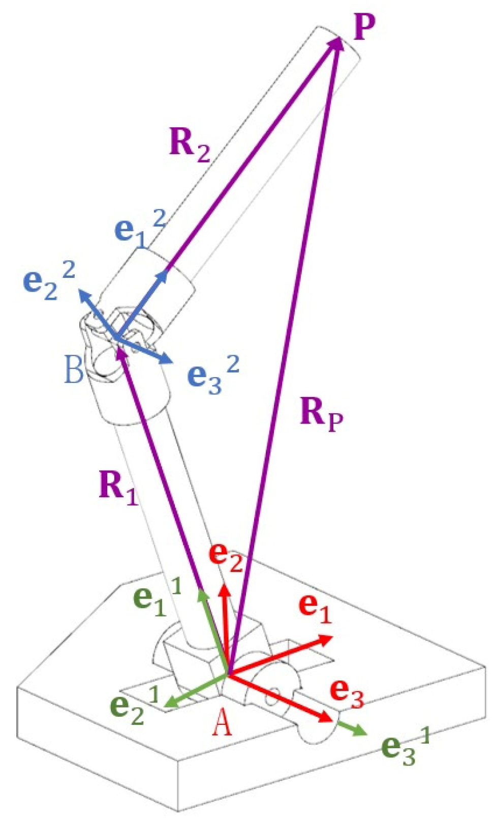
2.3.3. Configuration of Coupled Bodies

The objective of this section is to determine the relationships between the bases associated with coupled bodies. According to Figure 2, the links of a kinematic chain are represented by the vectors R₁, R₂∈ℜ³. The link R₁ is joined to the base by means of a rotational joint at point A. Link R₂ is joined to R₁ by means of a universal joint at point B. This allows modeling a general movement of the articulated links, which can then be applied to model mechanisms. To start the modeling process, a global reference system is first defined e_j and local reference systems e_jⁿ, j = 1, 2, 3 are defined over the links (see Figure 2). The position vector R_P and the vectors R₁, R₂ associated with the links are represented in ℜ⁴ as follows:

R_P = (0,x,y,z)
R₁ = r₁ e₁¹
R₂ = r₂ e₁²

(21)

Here, R₁, R₂, R_P ∈ℜ⁴, and r₁, r₂∈ℜ⁺ are the lengths of the links. Moreover, the bases e_jⁿ, j = 1, 2, 3 are orthogonal.

The modeling process is as follows:

The first step consists of determining the coordinates of point “P” shown in Figure 2 by means of the position vector R_P and the vectors R₁ and R₂. The vector R_P defines the position of the final end of the kinematic chain with respect to the global base e_j. This vector can be written as follows:

R_P = R₁ ⊕ R₂ = r₁ e₁¹ ⊕ r₂ e₁²

(22)

The second step consists of transforming the elements of the bases e₁¹ and e₁² to the canonical base e_j to obtain the vector R_P referenced to the global base. The cases of spatial and planar motion will be considered.

1. In the case of spatial movement, this is modeled through the composition of relative movements, and the bases are defined as follows:

e₁¹ = ρ(p₁, e₁)
 e₁² = ρ(q, e₁)

(23)

where

q = p₁∗p₂∗p₃

(24)

and where:

p₁ = (p₁₀, 0, 0, p₁₃)
 p₂ = (p₂₀, 0, 0, p₂₃)
 p₃ = (p₃₀, 0, p₃₂, 0)

(25)

2. For the case of motion in the plane, we have that p₂ = 0, and p₁ and p₃ have an axis of rotation in the z-axis. This movement can be modeled by the composition of relative movements or by mean absolute movements. For relative motion, the bases are defined as follows:

e₁¹ = ρ(p₁, e₁)
 e₁² = ρ(q, e₁)

(26)

Here,

q = p₁∗p₃

(27)

where

p₁ = (p₁₀, 0, 0, p₁₃)
 p₃ = (p₃₀, 0, 0, p₃₃)

(28)

For absolute motion, the bases are defined as follows:

e₁¹ = ρ(p₁, e₁)
 e₁² = ρ(p₃, e₁)

(29)

The last step consists of obtaining a general expression of Equation (22), and this is achieved by substituting, for the case of spatial movement, Equation (23) in Equation (22). This is as follows:

$$\begin{array}{ll}{\underset{\_}{\mathbf{R}}}_{\mathrm{P}}& ={\mathrm{r}}_1 \rho ({\mathbf{p}}_1 ,{\underset{\_}{\mathbf{e}}}_1)\oplus {\mathrm{r}}_2 \rho (\mathbf{q}, {\underset{\_}{\mathbf{e}}}_1)\\ & ={\mathrm{r}}_1\left({\mathbf{p}}_1\ast {\underset{\_}{\mathbf{e}}}_1\ast {\stackrel{\_}{\mathbf{p}}}_1\right)\oplus {\mathrm{r}}_2\left({\mathbf{p}}_1\ast {\mathbf{p}}_2\ast {\mathbf{p}}_3\ast {\underset{\_}{\mathbf{e}}}_1\ast \stackrel{\_}{{\mathbf{p}}_1\ast {\mathbf{p}}_2\ast {\mathbf{p}}_3}\right)\end{array}$$

(30)

2.4. Modeling of a RRR Planar Parallel Robot

This section presents the modeling of an RRR planar robot using the results of the previous sections. The formal definition of a parallel robot is as follows: A parallel robot is made up of an end-effector with n degrees of freedom, and of a fixed base, linked together by at least two independent kinematic chains. Motion is originated by n single actuators [54].

This definition is important because it has implications for the analysis and modeling of parallel robots. Modeling consists of determining a mathematical model by means of which it is possible to formulate the inverse kinematic problem. Figure 3 shows the RRR-type parallel robot with flat motion that is the subject of study in this research. To determine the degrees of freedom (DOFs) of the kinematic chain under study shown in Figure 3, the Grübler–Kutzbach criterion was applied [55]. Consequently, the robot has 3 DOFs.

The robot shown in Figure 3 consists of a mobile platform that moves freely along the work plane and six links, three of which are connected to three actuators, which provide movement, and three coupling links.

One of the first modeling steps consists of defining position vectors on each of the links composing the robot and associating vectors on points of interest, as shown in Figure 3. The links are classified into conductive or driving and driven. The former are connected to the ground and have an associated actuator that produces the movement, while the latter are connected to the moving platform. The robot configuration allows the formation of three vector loops.

The definition of the inverse kinematic problem related to the robot configuration shown in Figure 3 is as follows:

“Given the coordinates of the centroid of the moving platform and its angle of rotation measured with respect to the x-axis, find the angles of the links (conductive and driven) that make up the robot configuration shown in  Figure 3.”

The study of the parallel robot can be performed by modeling each vector loop separately. The steps to carry out the modeling are as follows:

(1)

Locate a coordinate system (x, y) and the fixed inertial base.

(2)

Select a kinematic chain (loop).

(3)

Associate vectors with each link of the selected kinematic chain.

(4)

Associate mobile bases for each rotation movement when going through the chain (Figure 4).

(5)

Construct the equation of position that locates the centroid of the platform with the origin (x, y).

(6)

Model the base rotations using expression (19).

(7)

Represent the position equation from step 5 in terms of quaternions.

(8)

Repeat the process for each of the remaining kinematic chains.

(9)

Formulate the inverse kinematic problem.

Figure 4 shows the inertial base and the moving bases associated with each link. Figure 5 shows the rotation angles of each link and of the mobile platform.

According to Figure 4, the bases or mobile systems are defined on the links that compose the robot with origin in each rotational joint, and the rotation angles of each chain are measured in relative terms (see Figure 5).

2.4.1. 3-RRR Robot Loop Equations

In this section, the loop equations related to each kinematic chain associated with the robot under study are generated. Each link is represented by the vectors R₂ⁱ, R₃ⁱ, R₄ⁱ∈ℜ³ on which the mobile bases e_j²ⁱ, e_j³ⁱ, and e_j⁴ⁱ are defined. Therefore, the position vector R_P∈ℜ³ that locates the platform centroid from the origin of the coordinates can be expressed in terms of the vector sum in ℜ⁴ for the case of the kinematic chains that make up the robot in the following way:

R₁ⁱ ⊕ R₂ⁱ ⊕ R₃ⁱ ⊕ R₄ⁱ = R_P

(31)

Furthermore, by considering unitary quaternions to represent the rotations of each link that make up each chain, unitary norm equations are generated. This is as follows:

  ‖p_2i‖² = 1
   ‖p_3i‖² = 1
   ‖p_4i‖² = 1

(32)

Each vector associated with the links can be represented in terms of its length and in the direction of a unitary vector, according to expressions (21), as follows:

R₁ⁱ = (0, x_i, y_i, 0)
 R₂ⁱ = r₂ⁱ e₁²ⁱ
 R₃ⁱ = r₃ⁱ e₁³ⁱ
 R₄ⁱ = r₄ⁱ e₁⁴ⁱ
 R_P = (0, x_P, y_P, 0)

(33)

where i = 1,2,3, in addition to r₂ⁱ, r₃ⁱ, and r₄ⁱ, are the lengths of the links. Each mobile base represents a rotation of the inertial base e_j (see Figure 4). Such rotations can be expressed in terms of relative quaternions. This is as follows:

e₁²ⁱ = ρ(q_2i, e₁); q_2i = p_2i
e₁³ⁱ = ρ(q_3i,e₁); q_3i = p_2i∗p_3i
e₁⁴ⁱ = ρ(q_4i, e₁); q_4i = p_2i∗p_3i∗p_4i
e_j⁵ⁱ = ρ(q_5i, e_j); q_5i = p_2i∗p_3i∗p_4i∗p_5i
e_j^P = ρ(q_P, e_j); q_P = p_P

(34)

or, in terms of absolute quaternions:

e₁²ⁱ = ρ(p_2i, e₁)
 e₁³ⁱ = ρ(p_3i, e₁)
 e₁⁴ⁱ = ρ(p_4i, e₁)
 e₁⁵ⁱ = ρ(s_5i, e₁); s_5i = p_4i∗p_5i

(35)

where

p_2i = (p_20i, 0, 0, p_23i)
 p_3i = (p_30i, 0, 0, p_33i)
 p_4i = (p_40i, 0, 0, p_43i)
 p_5i = (c(β_i/2), 0, 0, s(β_i/2))
 p_P = (c(θ_P/2), 0, 0, s(θ_P/2))

(36)

The quaternions p_2i, p_3i, and p_4i are associated with the angles θ_2i, θ_3i, and θ_4i. In addition, the quaternions p_2i, p_3i, and p_4i, allow the rotations of the first, second, and third link of each kinematic chain to be carried out.

2.4.2. Platform Orientation Equation

The mobile platform of the robot under study can be oriented in each movement. The orientation equation is obtained by considering the following equality:

e_j⁵ⁱ = e_j^P

(37)

For the case of relative quaternions, we have the following:

ρ(q_5i, e_j) = ρ(q_P, e_j)

(38)

if and only if

q_5i = q_P

(39)

Finally,

p_2i∗p_3i∗p_4i∗p_5i = p_P

(40)

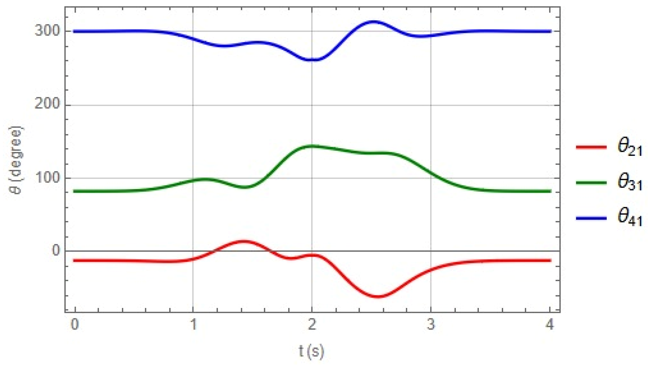
2.4.3. Formulation of the Inverse Kinematic Problem of the RRR Planar Parallel Robot

In this section, we formulate the inverse kinematic problem associated with the RRR parallel robot configuration shown in Figure 3. That is, “Given the coordinates of the centroid of the moving platform and the orientation of the base e_j^P (see Figure 4), find for j = 1,2,3 the angles (θ_2i, θ_3i, θ_4i) associated with the quaternions p_2i, p_3i, p_4i, such that Equations (31), (32) and (40) are satisfied”.

The formulation of the inverse problem of the RRR robot modeled with unitary quaternions generates a system of 21 nonlinear equations with 18 unknowns of the algebraic type.

For each loop, Equation (31) generates 2 algebraic equations in x and y, Equation (32) represents 3 unitary norm equations, and expression Equation (40) generates 2 other algebraic equations, so adding them together, 21 equations are obtained. Similarly, for each chain, there are six unknowns, which are the components of the quaternions p_2i, p_3i, and p_4i; that is, (p_2i0, p_2i3, p_3i0, p_3i3, p_4i0, p_4i3), and, therefore, there are 18 unknowns.

Once the quaternions p_2i, p_3i, and p_4i, have been calculated, the associated angles (θ_2i, θ_3i, and θ_4i) can be determined using the following relationships:

θ_2i = 2 tan⁻¹(p_2i3/p_2i0)
  θ_3i = 2 tan⁻¹(p_3i3/ p_3i0)
  θ_4i = 2 tan⁻¹(p_4i3/ p_4i0)

(41)

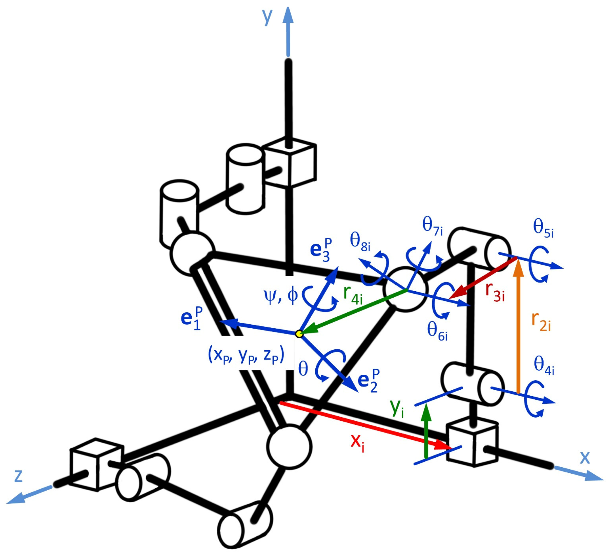
2.5. Modeling of a PRRS Spatial Parallel Robot

The objective of this section is to apply the unitary quaternion modeling methodology described in Section 2.3.3 to analyze the motions of a PRRS-type spatial parallel robot [35]. The robot under study has prismatic (P), rotational (R), and spherical (S) joints, which connect the links, as shown in Figure 6.

The robot shown in Figure 6 consists of three independent kinematic chains and a moving platform. The links that are connected to the ground of the system have associated prismatic joints (P) that move along the axes of a Cartesian system. Each chain has two links that are articulated by means of rotational joints (R), and, finally, the connection of the links with the mobile platform is by means of a spherical joint (see Figure 6).

The objective of the study is to determine a mathematical model that allows formulating the inverse kinematic problem associated with the configuration of the robot.

2.5.1. 3-PRRS Robot Loop Equations

According to Figure 6, to locate the coordinates of point “P” located at the centroid of the mobile platform from the origin of coordinates of the entire system, the closed-loop equations must be formulated. These expressions are obtained by means of the following vector equation:

R_1xⁱ ⊕ R_1yⁱ ⊕ R₂ⁱ ⊕ R₃ⁱ ⊕ R₄ⁱ = R_P

(42)

When considering unitary quaternions to model the rotations of the links with R- and S-type connections that make up each chain, unitary norm equations are generated. This is as follows:

‖p_4i‖² = 1
 ‖p_5i‖² = 1
 ‖p_6i‖² = 1
 ‖p_7i‖² = 1
 ‖p_8i‖² = 1

(43)

The vectors associated with the links that make up the robot under study can be written in terms of the local bases shown in Figure 7.

R_1xⁱ = xⁱ e₁¹ⁱ
 R_1yⁱ = yⁱ e₂¹ⁱ
 R₂ⁱ = r₂ⁱ e₂²ⁱ
 R₃ⁱ = r₃ⁱ e₂³ⁱ
 R₄ⁱ = r₄ⁱ e₁⁴ⁱ
 R_P = (0, x_P, y_P, z_P)

(44)

The local or mobile bases shown in Figure 7 can be written in terms of quaternions and as a function of the inertial or canonical basis as follows:

e_j¹ⁱ = ρ(q_1i, e₁); q_1i = p_1i∗p_2i∗p_3i
e₂²ⁱ = ρ(q_2i, e₁); q_2i = q_1i∗p_4i
e₂³ⁱ = ρ(q_3i,e₁); q_3i = q_2i∗p_5i
e₁⁴ⁱ = ρ(q_4i, e₁); q_4i = q_3i∗p_6i∗p_7i∗p_8i
e_j⁵ⁱ = ρ(q_5i, e_j); q_5i = q_4i∗p_9i
e_j^P = ρ(q_P, e_j) q_P = p_ψ∗p_θ∗p_ϕ

(45)

The configuration of each quaternion in terms of the rotation angles shown in Figure 8 is expressed as follows:

p_1i = (c(β_1i/2), 0, s(β_1i/2), 0)
 p_2i = (c(β_2i/2), 0, 0, s(β_2i/2))
 p_3i = (c(β_3i/2), s(β_3i/2), 0, 0)
 p_4i = (p_40i, p_41i, 0, 0)
 p_5i = (p_50i, p_51i, 0, 0)
 p_6i = (p_60i, 0, 0, p_63i)
 p_7i = (p_70i, 0, p_72i, 0)
 p_8i = (p_80i, 0, 0, p_83i)
 p_9i = (c(β_9i/2), 0, 0, s(β_9i/2))
 p_ψ = (c(ψ/2), 0, 0, s(ψ/2))
 p_θ = (c(θ/2), 0, s(θ/2), 0)
 p_ϕ = (c(ϕ/2), 0, 0, s(ϕ/2))

(46)

The rotation angles shown in Figure 8 are associated with the moving bases of each kinematic chain that integrates the robot and are defined, like the RRR robot, in relative terms.

2.5.2. Equation of Platform Orientation

To complete the modeling of the robot under study, it is necessary to construct the equations to define the orientation of the mobile platform. These equations are obtained considering the following equality:

e_j⁵ⁱ = e_j^P

(47)

Being

ρ(q_5i, e_j) = ρ(q_P, e_j)

(48)

and

q_5i = q_P

(49)

then

p_1i∗p_2i∗p_3i∗p_4i∗p_5i∗p_6i∗p_7i∗p_8i∗p_9i = p_ψ∗p_θ∗p_ϕ

(50)

2.5.3. Formulation of the PRRS-Type Inverse Problem

In this section, we formulate the inverse kinematic problem related to the PRRS robot configuration shown in Figure 6. That is, “Given the coordinates of the centroid of the moving platform and the angles (ψ,θ,ϕ), which define the position of the origin and the orientation of the base e_j^P (see Figure 8), find for j = 1,2,3, the magnitudes xⁱ and the angles (θ_4i, θ_5i, θ_6i, θ_7i, θ_8i) associated with the quaternions p_4i, p_5i, p_5i, p_6i, p_7i, p_8i, such that Equations (42), (43) and (50) are satisfied”.

The formulation of the inverse problem of the PRRS robot modeled with unitary quaternions generates a system of 36 nonlinear equations with 33 unknowns of the algebraic type.

For each loop, Equation (42) generates 3 algebraic equations in x, y, and z, while Equation (43) represents 5 unit norm equations, and expression (50) generates another 4 algebraic equations, giving a total of 36 equations. Similarly, for each loop, there are 11 unknowns, which are the components of the quaternions p_4i, p_5i, p_5i, p_6i, p_7i, and p_8i, that is, (p_40i, p_41i, p_50i, p_51i, p_60i, p_63i, p_70i, p_72i, p_80i, p_83i) and the displacement xⁱ of the prismatic joint.

Once the quaternions p_4i, p_5i, p_5i, p_6i, p_7i, and p_8i are calculated, the associated angles (θ_4i, θ_5i, θ_6i, θ_7i, and θ_8i) can be determined by means of the following relations:

θ_4i = 2 tan⁻¹(p_41i/p_4i0)
 θ_5i = 2 tan⁻¹(p_51i/p_50i)
 θ_6i = 2 tan⁻¹(p_63i/p_60i)
 θ_7i = 2 tan⁻¹(p_72i/p_70i)
 θ_8i = 2 tan⁻¹(p_83i/p_80i)

(51)

2.6. Numerical Experimentation

In this section, the numerical experimentation for the solution of the inverse kinematic problems of both robots is presented. To solve the systems of equations associated with the inverse kinematic problems of both robots (which turned out to be nonlinear and nonsquare), the nonlinear programming algorithm BFGS was used [46].

The Davidon–Fletcher–Powell (DFP) method is a quasi-Newton method that is used to find the unconstrained minimum of a differentiable function “f” of several variables and consists of generating successive approximations of the inverse of the Hessian of the function under study. The DFP method has been and remains a widely used gradient technique. The method tends to be robust; that is, it typically tends to perform well on a wide variety of practical problems and was first proposed by Davidon [56] and later reformulated by Fletcher and Powell [57]. A variant or improvement of the DFP is the BFGS algorithm [33,34], which is currently considered the most efficient of all quasi-Newton update formulas and is a computational iterative technique used to solve nonlinear optimization problems by using the first derivative and the Hessian matrix of the objective function [58]. The DFP update formula is effective but is outperformed by the BFGS formula [33,59]. In this paper, we propose the objective functions associated with the position kinematics of each robot studied and use the BFGS algorithm, which is automated in the Mathematica V12 formal computation library [46].

3. Results

This section presents the results obtained by solving the mathematical models of the robots studied in this work. An objective function and a trajectory are proposed for each analysis.

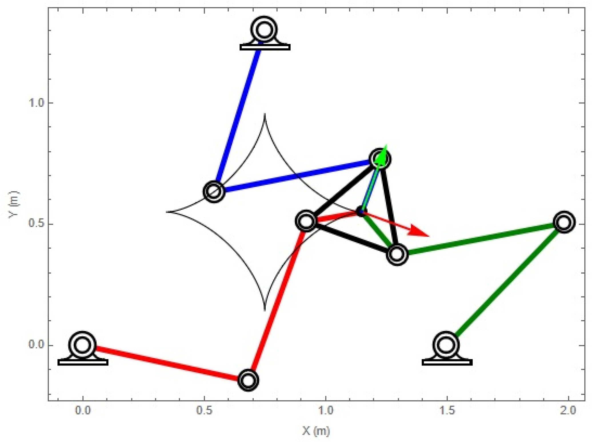
3.1. Numerical Model and Solution for the RRR Parallel Robot

The inverse problem of the RRR planar parallel robot generated a system of 21 nonlinear equations with 18 polynomial unknowns. To use the BFGS algorithm in the solution of the inverse problem related to the RRR-type robot, the following objective function was proposed:

$$F={\sum }_{i=1}^3\left({\sum }_{j=2}^3{({\underset{\_}{\mathbf{R}}}_1^i\oplus {\underset{\_}{\mathbf{R}}}_2^i\oplus {\underset{\_}{\mathbf{R}}}_3^i\oplus {\underset{\_}{\mathbf{R}}}_4^i-{\underset{\_}{\mathbf{R}}}_{\mathbf{P}})}_{ij}^2+{\sum }_{k=2}^4{({‖{\mathbf{p}}_{ki}‖}^2-1)}_{ik}^2+{\sum }_{l=1}^4{({\mathbf{p}}_{2i}\ast {\mathbf{p}}_{3i}\ast {\mathbf{p}}_{4i}\ast {\mathbf{p}}_{5i}-{\mathbf{p}}_{\mathrm{P}})}_{il}^2 \right)$$

(52)

Here, i = kinematic chain, j; l = component of the vector; and k = quaternion.

To solve the model, one trajectory was considered, and the interval was 0 ≤ t ≤ 4 s. That is,

s = 2π(10(t/4)³ − 15(t/4)⁴ + 6(t/4)⁵)
x_P = 0.75 + 0.4 cos(s)³
y_P = 0.55 + 0.4 sin(s)³

(53)

The following intervals are defined for platform orientation:

If 0 ≤ t < 2, then θ_P = s/6 − π/9
If 2 ≤ t ≤ 4, then θ_P = (2π − s)/6 − π/9

The initial configuration of the robot type RRR and the graph of the geometric place of the trajectory are shown in Figure 9.

Equation (52) was solved using the BFGS algorithm. The results obtained are plotted in the following figures.

Figure 10, Figure 11 and Figure 12 show the angular displacements associated with each kinematic chain integrating the robot calculated within the proposed time interval in the trajectory.

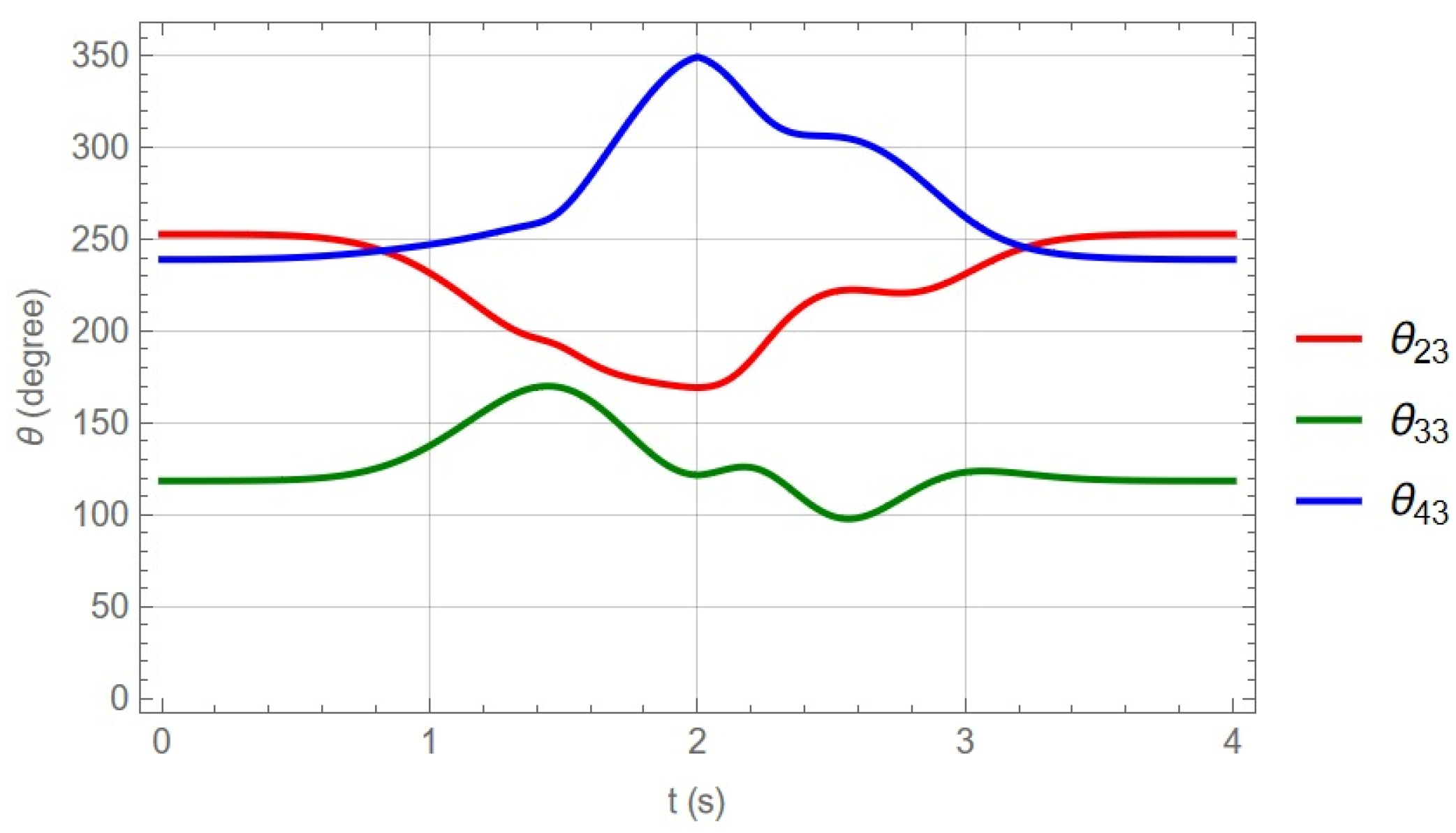
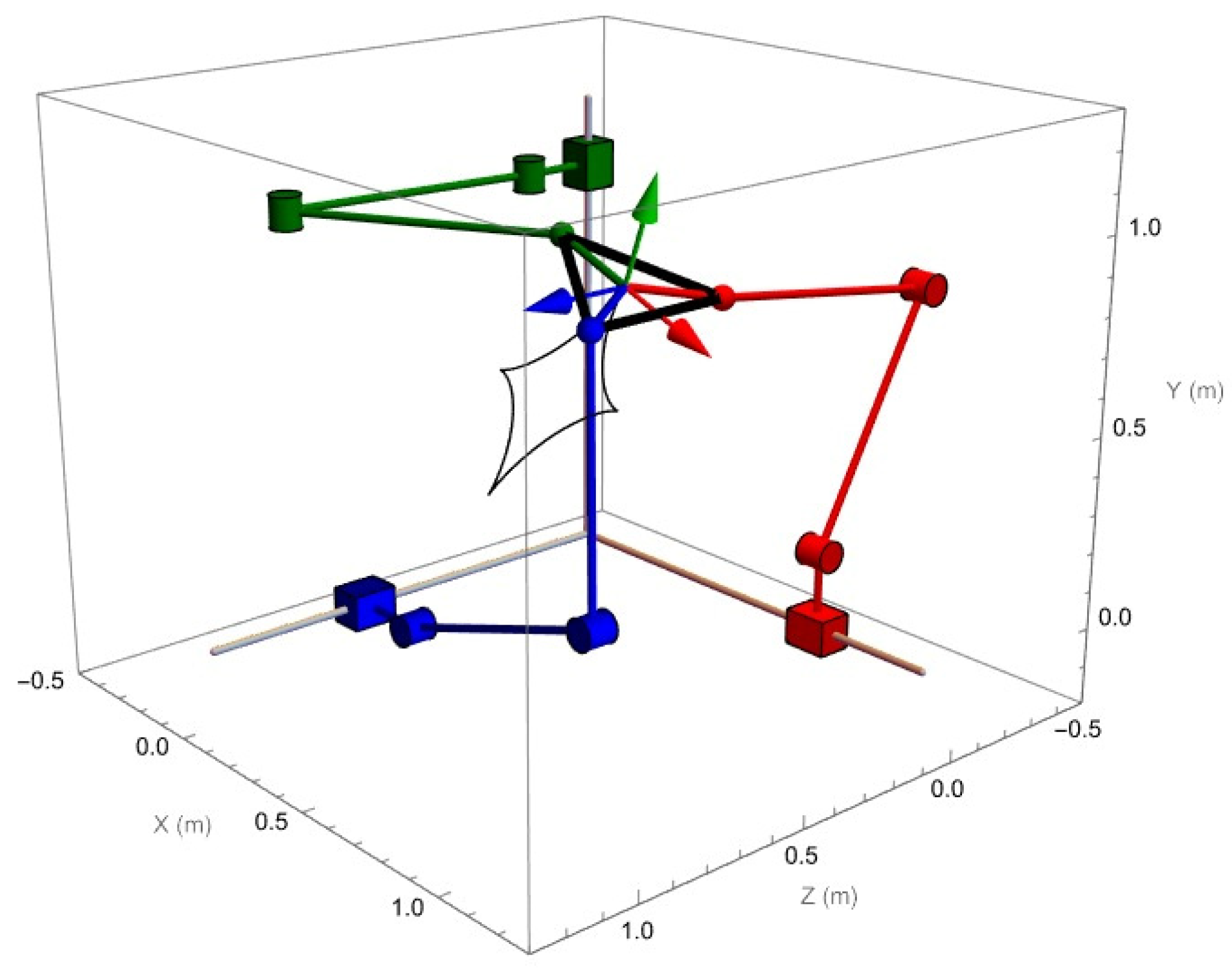
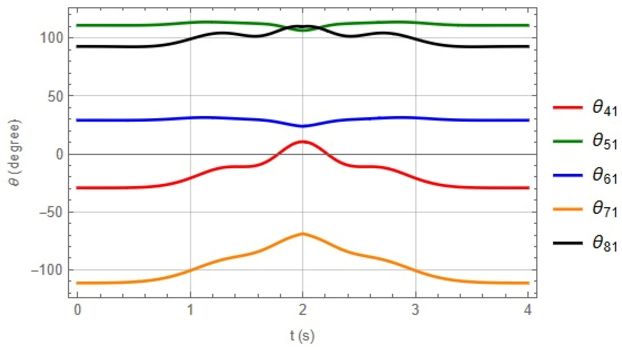
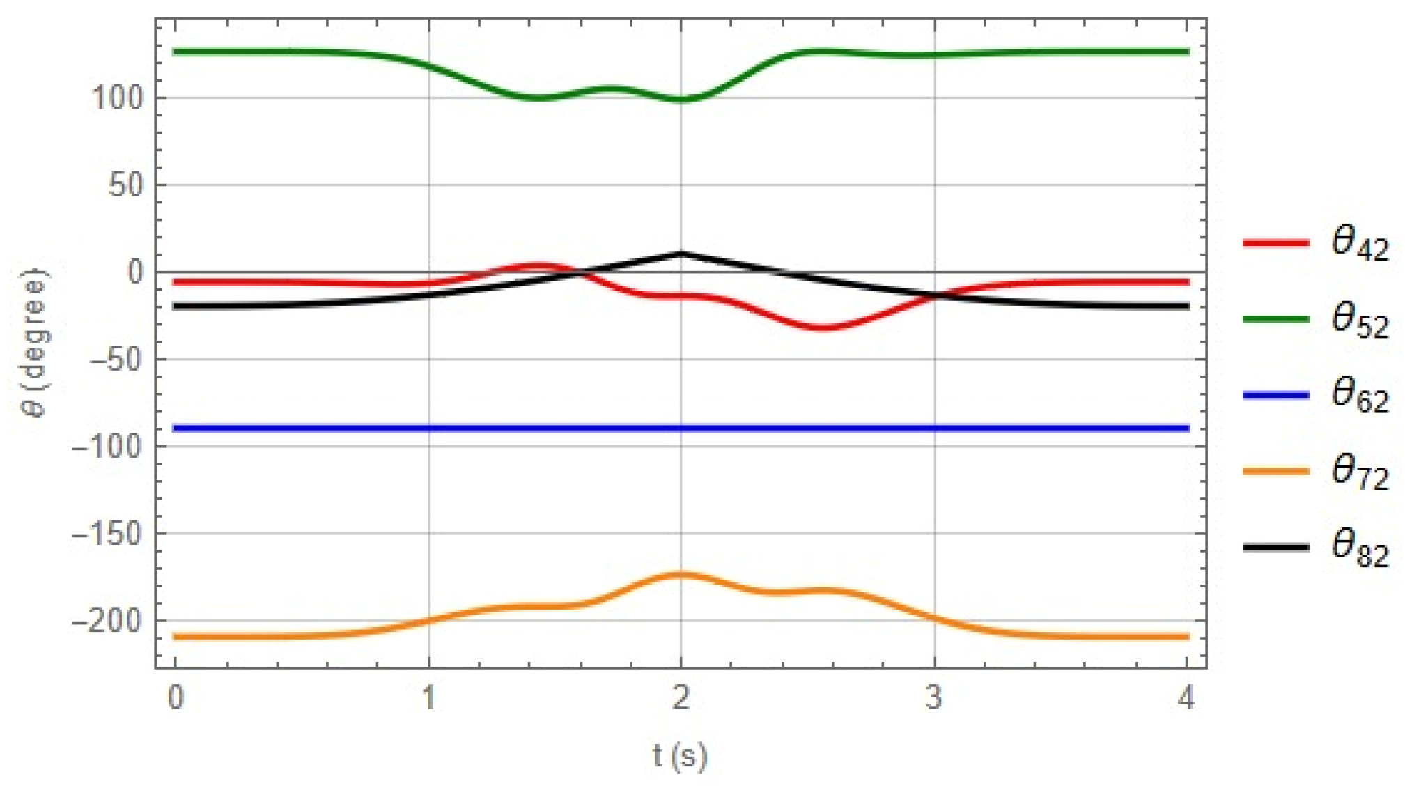
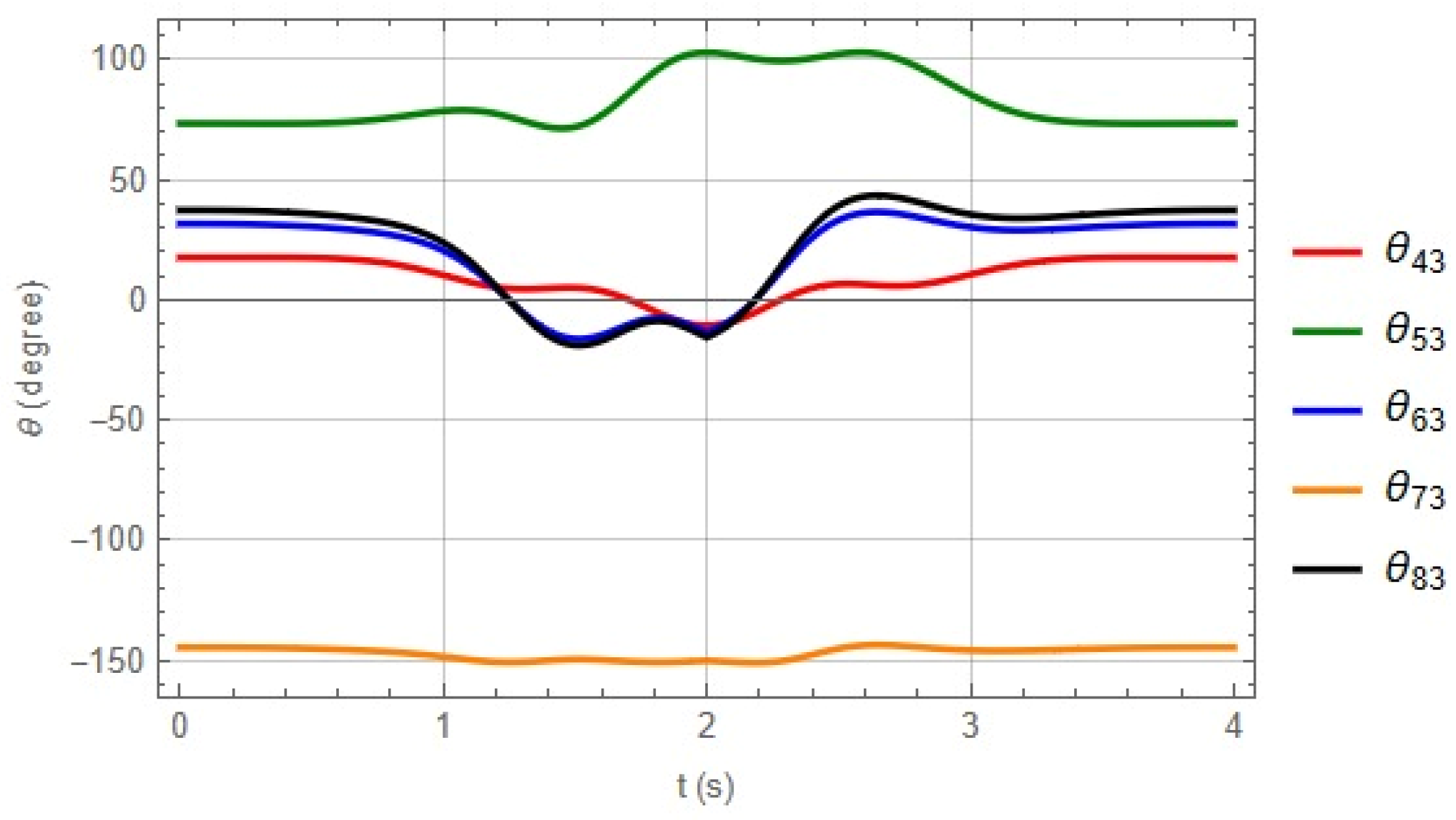
3.2. Numerical Model and Solution for the PRRS Parallel Robot

The mathematical model related to the PRRS robot consists of 36 nonlinear equations and 33 unknowns for each kinematic chain. To use the BFGS algorithm in the solution of the inverse problem related to the robot configuration shown in Figure 8, the following objective function was proposed:

$$\begin{gathered} F={\sum }_{i=1}^3\left({\sum }_{j=2}^4{\left({\underset{\_}{\mathbf{R}}}_{1\mathrm{x}}^i\oplus {\underset{\_}{\mathbf{R}}}_{1\mathrm{y}}^i\oplus {\underset{\_}{\mathbf{R}}}_2^i\oplus {\underset{\_}{\mathbf{R}}}_3^i\oplus {\underset{\_}{\mathbf{R}}}_4^i-{\underset{\_}{\mathbf{R}}}_{\mathbf{P}}\right)}_{ij}^2+{\sum }_{k=4}^8{\left({‖{\mathbf{p}}_{ki}‖}^2-1\right)}_{ik }^2+ \\ {\sum }_{l=1}^4{({\mathbf{p}}_{1i}\ast {\mathbf{p}}_{2i}\ast {\mathbf{p}}_{3i}\ast {\mathbf{p}}_{4i}\ast {\mathbf{p}}_{5i}\ast {\mathbf{p}}_{6i}\ast {\mathbf{p}}_{7i}\ast {\mathbf{p}}_{8i}\ast {\mathbf{p}}_{9i}-{\mathbf{p}}_{\psi }\ast {\mathbf{p}}_{\theta }\ast {\mathbf{p}}_{\Phi })}_{il}^2\right) \end{gathered}$$

(54)

where i = kinematic chain, j; l = component of the vector; and k = quaternion.

To visualize the movements of the robot, a trajectory and the time interval 0 ≤ t ≤ 4 s was proposed. That is,

s = 2π(10(t/4)³ − 15(t/4)⁴ + 6(t/4)⁵)
x_P = 0.75 + 0.2 sin(s)³
y_P = 0.75 + 0.2 cos(s)³
z_P = 0.75 − 0.2 cos(s)³

The following intervals are defined for platform orientation:

If 0 ≤ t < 2 then ψ = s/6 − π/9
If 2 ≤ t ≤ 4 then ψ = (2π − s)/6 − π/9
θ = 0
ϕ = 0

The initial configuration of the robot and the graph of the geometric place of the trajectory are shown in Figure 13.

Equation (54) was solved using the BFGS algorithm. The results obtained are plotted in the following figures.

Figure 14, Figure 15 and Figure 16 show the angular displacements associated with each kinematic chain that integrates the robot, and Figure 17 shows the displacements in the Cartesian axes, calculated in the time interval proposed in the trajectory.

4. Discussion

The methodology presented in this article made it possible to generate the inverse kinematic models of the RRR and PRRS parallel robots in a systematic manner so that this methodology can be applied to various configurations and types of parallel kinematic chains. The methodological proposal took into consideration the systematization of the quaternion algebra developed by Reyes [25] and applied by Jiménez et al. [24]. The kinematic modeling of the position was a function of the unknown quaternion parameters.

The binary operations defined by the expressions (1) and the linear transformation described by Equation (12) allowed us to establish the kinematic modeling in a vectorial way by means of loop equations and platform orientation equations as a multiplication of quaternions representing relative spins in x, y, and z axes. The kinematic modeling developed with the method proposed in this work does not require matrix representations, nor does it take into account in its development the trigonometric functions defined between the parameters of the quaternions given by Equation (15), which produces highly nonlinear polynomial equations, which were solved numerically to obtain the parameters or components of the quaternions. On the other hand, the movements of the moving platform of the PRRS robot were represented by 3 quaternions associated with the 3 DOFs required for its orientation, although a general quaternion can also be used, as was the case presented in [28,29].

It should be noted that the mathematical models associated with the inverse kinematic problems of each robot were solved by applying the Broyden–Fletcher–Goldfarb–Shanno method [46], which is automated in Mathematica V12 software. With the obtained solutions, it was possible to plot the movements of the robots (see Figure 9 and Figure 13). Two trajectories were taken into account to solve the inverse kinematic problem for each robot and the calculation was performed to determine the rotations of the RRR robot and the translations and rotations of the PRRS robot.

A methodology similar to that of the present work was proposed by Jiménez et al. [24]. It is possible to find four important differences between the methodology proposed in this paper and the modeling method developed by Jiménez et al. [24]: the first difference is presented in the study of the movements, since in [24], sequences of rotations were used and the axes of rotation of each rotation were updated in the modeling of the movements of an anthropomorphic RRR robot, while in the modeling of parallel robots developed in this article, it was not required to update the axes of rotations, since this process is performed by multiplying quaternions when representing relative spins, resulting in a reduction in operations. The second difference is in the modeling of the robot configurations, since in [24], the initial and final positions of the robot were considered for the construction of the model, while to develop the models of the parallel robots of the present study, only the initial position was required, thus simplifying the modeling of the kinematics. The third difference is presented in the configuration of the mathematical models, since in the work developed by Jiménez et al. [24], systems of square equations were formed (same number of equations and unknowns), while the modeling proposed in this article generated systems of nonlinear, nonsquare equations, due to the fact that the equation representing the platform orientation is constituted by a multiplication of quaternions that generates four-element vectors and produces extra equations. The advantage of having the orientation equation is that it allows us to calculate the angles at all joints. The fourth difference is in the numerical method used, since in [24], having a square system of equations and unknowns, the Newton–Raphson method was used to obtain the numerical solution of the kinematics of a 3 DOF PUMA robot, and, in the present study, the Broyden–Fletcher–Goldfarb–Shanno quasi-Newton method was applied to solve the rectangular systems of equations of each robot studied.

For the generalization of the modeling method with unitary quaternions presented in this article, it is necessary to include in future works the study of some more complex configurations of parallel robots, as is the case of the Stewart Platform and the Delta Space Robot [60,61], in order to know the efficiency and scope of the modeling method. In the same way, it will be necessary to apply the modeling method proposed in this article in conjunction with other proven methodologies, such as the Denavit–Hartenberg methodology [62], in order to know the positive or negative implications of the kinematic analysis. The D-H method is widely used in open-chain robot modeling, and although its application in parallel robots is not so popular, there are some important studies where this method has been applied, for example, in a recent research the D-H method was used to model a Spatial Delta Robot as a basis for applying the interior point algorithm optimization method to assign tolerances to the geometric parameters of the robot [63] and in another work the Denavit-Hartenberg method of the Lie group was applied to model the kinematics of a Hexapod Parallel Manipulator Robot [64].

On the other hand, the unitary quaternion modeling used in this paper has some disadvantages, such as the following:

• Quaternions can be considered abstract mathematical manipulations, and it can be understood that they have no direct physical meaning with rigid body rotations.
• One of the limitations of the modeling presented in this research is the analysis of the kinematics since it was developed using a quaternion com-position to express the orientations of a link with respect to the previous one, which generated a system of more equations than unknowns (parameters: p0, p1, p2, p3). It is possible to rewrite the vector loop equations to eliminate unknown quaternions and obtain an equal number of equations and unknowns.
• No established model of coordinate system assignment was followed, which allowed us to adjust to the specific problem, although other assignment methods, such as basic matrices [65], can be used, since both include translation and orientation information.
• The position and orientation equations, together with the quaternion norms, generate a system of nonlinear equations, which implies that the modeling method is highly dependent on numerical methods. This problem is also often encountered by some methods using Euler parameters [66] when solving the initial position of spatial mechanisms by the Broyden–Fletcher–Goldfarb–Shanno numerical method.
• The quaternion parameters are not independent since they must satisfy a normalization constraint, adding one more equation to the system of equations.

Modeling with quaternions has the following advantages:

• In this research, only one quaternion was used for each transformation, representing one axis orientation to obtain the coordinate system attached to each link.
• The kinematics was performed using vector equations of position and orientation, and these equations can be preserved for analysis with higher derivatives. A relevant fact in this work was that the equations that represented the orientations of the mobile platforms of the 3-RRR and 3-PRRS robots were of the vectorial type, when they are commonly represented in matrix form.

Despite its applications, some authors have pointed out that the D-H method presents some problems, such as the following:

• The modeling is relatively complicated since four transformations given by homogeneous matrices are required to obtain the coordinate system attached to each link.
• The use of rotations and translations on the x and z axes limits the modeling, and some parameters, such as distances or fixed angles, are not necessary to represent links and joints, as in the case of spherical joints.
• A disadvantage of the D-H method is the necessity of defining coordinate systems following a convention instead of fitting the specific problem.
• Some serious problems may arise when applying D-H in kinematic error calibration [67].

The D-H methodology has some important advantages, such as the following:

• The advantage of the D-H matrix method is its conceptual comprehensibility, allowing the user to describe complex systems of multibody systems in a straightforward manner with basic knowledge of matrix operations and their derivatives.
• Algorithms have been developed for the kinematics of open and closed loop systems. In addition, different types of kinematic joints commonly used in robots and mechanisms have been modeled with this method [68].
• In the same way, there are numerical methods developed for the solution of the equations obtained by constructing the equations of the matricial loops [68].

Finally, the development of new modeling methods that include an integration of D-H methodology and unitary quaternion modeling methods could improve the kinematic and dynamic analysis of parallel robots.

5. Conclusions

In this article, a methodology to model a rigid multibody in the plane and in space using unit quaternions was presented. The methodology was used to model the movements of two parallel robots. The main conclusions are summarized in the following points:

• The methodology proposed in this work and the application of unitary quaternions in the modeling process made it possible to build in a systematic and functional way the mathematical models that define the inverse kinematic problem of a flat RRR-type robot and a PRRS-type space robot.
• The mathematical models obtained by applying the methodology to each robot had the following characteristics: (1) the inverse kinematic problem associated with the RRR robot generated a system of 21 nonlinear equations with 18 polynomial-type unknowns, and (2) the inverse kinematic problem associated with the PRRS robot generated a system of 36 nonlinear equations with 33 polynomial-type unknowns.
• To solve the mathematical models generated from the inverse kinematic problem approach in both robots, two linear and angular trajectories were used, and the Broyden–Fletcher–Goldfarb–Shanno numerical method was used to calculate the parameters of the quaternions that define the rotations and displacements of each joint. The BFGS optimization method was used due to the high number of equations and unknowns related to the mathematical models of both robots and the advantage offered by formal calculation packages such as Mathematica V12, which has a such method programmed.
• The systematization of unitary quaternions developed by Reyes [25] and applied by Jiménez et al. [24] in the modeling of a PUMA robot allowed the construction of kinematic models of parallel robots using the binary operations of addition and multiplication between quaternions. Thus, it was possible to model open and closed kinematic chains in a systematic way, which increases the scope of the theory developed by [25].
• To improve and apply the methodology presented in this work, it will be necessary to model parallel robots with complex configurations, such as cable-driven parallel robots [69]. In addition, it will be necessary to compare the unitary quaternion methodology with other methodologies, such as the screw theory [70], in order to know their differences and similarities.

The methodology presented in this paper can be extended to the complete kinematic study of parallel robots by incorporating the velocity, acceleration, and higher derivative models, and with them, it will be possible to model the dynamics of parallel robots. Likewise, it will be possible to study the direct kinematic problem and mechanism synthesis problems by using and improving the methodology.

References

1. Pott, A.; Hiller, M. Kinematic Modeling, Linearization and First-Order Error Analysis. In Parallel Manipulators, Towards New Applications, 1st ed.; Wu, H., Ed.; Intechopen: Rijeka, Croatia, 2008; pp. 155–174. [Google Scholar] [CrossRef]
2. Merlet, J.; Gosselin, C. Parallel Mechanisms and Robots. In Springer Handbook of Robotics, 1st ed.; Siciliano, B., Khatib, O., Eds.; Springer: Berlin, Heidelberg, 2008; pp. 269–285. [Google Scholar]
3. Himam, S.; Satish, G.; Subba, N.V. Relative Kinematic Analysis of Serial and Parallel Manipulators. In IOP Conference Series: Materials Science and Engineering; IOP Publishing: Bristol, England, 2018; Volume 455, p. 012040. [Google Scholar] [CrossRef]
4. Olarra, A.; Axinte, D.; Uriarte, L.; Bueno, R. Machining with the WalkingHex: A walking parallel kinematic machine tool for in situ operations. CIRP Ann. 2017, 66, 361–364. [Google Scholar] [CrossRef]
5. Baptiste, J. On the Improvements of a Cable-Driven Parallel Robot for Achieving Additive Manufacturing for Construction. In Cable-Driven Parallel Robots. Mechanisms and Machine Science; Gosselin, C., Cardou, P., Bruckmann, T., Pott, A., Eds.; Springer: Cham, Switzerland, 2018; Volume 53, pp. 353–363. [Google Scholar] [CrossRef]
6. Li, P.; Shu, T.; Wen, X.; Tian, W. Dynamic Visual Servoing of A 6-RSS Parallel Robot Based on Optical CMM. J. Intell. Robot. Syst. 2021, 102, 40. [Google Scholar] [CrossRef]
7. Ersoy, O.; Yildirim, M.C.; Ahmad, A.; Yirmibesoglu, O.D.; Koroglu, N.; Bebek, O. Design and Kinematics of a 5-DOF Parallel Robot for Beating Heart Surgery. In Proceedings of the 2019 IEEE 4th International Conference on Advanced Robotics and Mechatronics (ICARM), Toyonaka, Japan, 12 September 2019; pp. 274–279. [Google Scholar] [CrossRef]
8. Vaida, C.; Birlescus, I.; Pisla, A.; Ionut, U.; Tarnita, D.; Carbone, J. Systematic Design of a Parallel Robotic System for Lower Limb Rehabilitation. IEEE Access 2020, 8, 34522–34537. [Google Scholar] [CrossRef]
9. Chang, Z.; Yue, F. Design and Analysis for a Three-Rotational-DOF Flight Simulator of Fighter-Aircraft. Chin. J. Mech. Eng. 2018, 31, 55. [Google Scholar] [CrossRef]
10. Wang, S.; Zheng, K.; Chen, Y.; Xu, M.; Wang, D. DOF and kinematics analysis of a 3-UPU parallel mechanism for telescope secondary mirror support. In AOPC 2021: Novel Technologies and Instruments for Astronomical Multi-Band Observations, 120690C; SPIE: Bellingham, WA, USA, 2021. [Google Scholar] [CrossRef]
11. Sholanov, K.S. Kinematics of One-Loop Parallel Manipulators. In Parallel Manipulators of Robots. Mechanisms and Machine Science; Springer: Cham, Switzerland, 2021; Volume 92, pp. 67–87. [Google Scholar] [CrossRef]
12. Zhang, Y.; Han, H.; Zhang, H.; Xu, Z.; Xiong, Y.; Han, K.; Li, Y. Acceleration analysis of 6-RR-RP-RR parallel manipulator with offset hinges by means of a hybrid method. Mech. Mach. Theory 2022, 169, 104661. [Google Scholar] [CrossRef]
13. Hamdoun, O.; El Bakkali, L.; Zahra, F. Analysis and Optimum Kinematic Design of a Parallel Robot. Procedia Eng. 2017, 181, 214–220. [Google Scholar] [CrossRef]
14. Yao, S.; Li, H.; Zeng, L.; Zhang, X. Vision-based adaptive control of a 3-RRR parallel positioning system. Sci. China Technol. Sci. 2018, 61, 1253–1264. [Google Scholar] [CrossRef]
15. Baron, N.; Philippides, A.; Rojas, N. A Geometric Method of Singularity Avoidance for Kinematically Redundant Planar Parallel Robots. In Advances in Robot Kinematics. ARK 2018; Springer Proceedings in Advanced Robotics; Lenarcic, J., Parenti, V., Eds.; Springer: Cham, Switzerland, 2019; Volume 8, pp. 187–194. [Google Scholar] [CrossRef]
16. Meng, Q.; Xie, F.; Liu, X.; Takeda, Y. Screw Theory-Based Motion/Force Transmissibility Analysis of High-Speed Parallel Robots with Articulated Platforms. J. Mech. Robot. 2020, 12, 041011. [Google Scholar] [CrossRef]
17. Chai, X.; Wang, M.; Xu, L.; Ye, W. Dynamic Modeling and Analysis of a 2PRU-UPR Parallel Robot Based on Screw Theory. IEEE Access 2020, 8, 78868–78878. [Google Scholar] [CrossRef]
18. Jiménez, E.; Servín de la Mora, D.; Servín de la Mora, R.; Ochoa, F.; Acosta, M.; Luna, G. Modeling in Two Configurations of a 5R 2-DoF Planar Parallel Mechanism and Solution to the Inverse Kinematic Modeling Using Artificial Neural Network. IEEE Access 2021, 9, 68583–68594. [Google Scholar] [CrossRef]
19. Thiruvengadam, S.; Tan, J.S.; Miller, K.A. Generalised Quaternion and Clifford Algebra Based Mathematical Methodology to Effect Multi-stage Reassembling Transformations in Parallel Robots. Adv. Appl. Clifford Algebras 2021, 31, 39. [Google Scholar] [CrossRef]
20. Xiang, Y.; Li, Q.; Jiang, X. Dynamic rotational trajectory planning of a cable-driven parallel robot for passing through singular orientations. Mech. Mach. Theory 2021, 158, 104223. [Google Scholar] [CrossRef]
21. Noppeney, V.; Boaventura, T.; Siqueira, A. Task-space impedance control of a parallel Delta robot using dual quaternions and a neural network. J. Braz. Soc. Mech. Sci. Eng. 2021, 43, 440. [Google Scholar] [CrossRef]
22. Liu, K.; Kong, X.; Yu, J. Operation mode analysis of lower-mobility parallel mechanisms based on dual quaternions. Mech. Mach. Theory 2019, 152, 103577. [Google Scholar] [CrossRef]
23. Dantam, N. Robust and efficient forward, differential, and inverse kinematics using dual quaternions. Int. J. Rob. Res. 2020, 40, 1087–1105. [Google Scholar] [CrossRef]
24. Jiménez, E.; Servín de la Mora, D.; Reyes, L.; Servín de la Mora, R.; Melendez, J.; López, A.A. Modeling of Inverse Kinematic of 3-DoF Robot, Using Unit Quaternions and Artificial Neural Network. Robotica 2021, 39, 1230–1250. [Google Scholar] [CrossRef]
25. Reyes, R. Quaternions: Une Representation Parametrique Systematique Des Rotation Finies. Partie I: Le Cadre Theorique. In Rapport de Recherche 1303; INRIA: Rocquencourt, France; Le Chesnay, France, 1990. [Google Scholar]
26. Reyes, R. Quaternions: Une Representation Parametrique Systematique Des Rotation Finies. Partie II: Quelques Application. In Rapport de Recherche 1454; INRIA: Rocquencourt, France; Le Chesnay, France, 1991. [Google Scholar]
27. Murray, A.; Pierrot, F.; Dauchez, P.; McCarthy, J. A planar quaternion approach to the kinematic synthesis of a parallel manipulator. Robotica 1997, 15, 361–365. [Google Scholar] [CrossRef]
28. Ruggiu, M.; Kong, X. Reconfiguration Analysis of a 3-DOF Parallel Mechanism. Robotics 2019, 8, 66. [Google Scholar] [CrossRef]
29. Liu, Y.; Wu, H.; Liu, H.; Chen, B.; Yao, J.; Wang, Y. Forward kinematics for 6-UPS parallel robot using extra displacement sensor. J. Adv. Mech. Des. Syst. Manuf. 2018, 12, JAMDSM0130. [Google Scholar] [CrossRef]
30. Birlescu, I.; Husty, M.; Vaida, C.; Gherman, B.; Tucan, P.; Pisla, D. Joint-Space Characterization of a Medical Parallel Robot Based on a Dual Quaternion Representation of SE(3). Mathematics 2020, 8, 1086. [Google Scholar] [CrossRef]
31. Dong, G.Y.; Du, Y.H.; Li, W.P. A Forward Solution Algorithm of 6RUS Parallel Mechanism Based on Dual Quaternion Method. Int. J. Aerosp. Eng. 2023, 2023, 8617435. [Google Scholar] [CrossRef]
32. Nigatu, H.; Kim, D. Optimization of 3-DoF Manipulators’ Parasitic Motion with the Instantaneous Restriction Space-Based Analytic Coupling Relation. Appl. Sci. 2021, 11, 4690. [Google Scholar] [CrossRef]
33. Kumar, A.; Parhi, D. Dynamic walking of multi-humanoid robots using BFGS Quasi-Newton method aided Artificial potential field approach for uneven terrain. Soft Comput. 2022, 33, 5893–5910. [Google Scholar] [CrossRef]
34. Xie, S.; Sun, L.; Wang, Z.; Chen, G. A speedup method for solving the inverse kinematics problem of robotic manipulators. Int. J. Adv. Robot. Syst. 2022, 19, 17298806221104602. [Google Scholar] [CrossRef]
35. Haibo, Q.; Yuefa, F.; Sheng, G. Theory of Degrees of Freedom for Parallel Mechanisms with Three Spherical Joints and Its Applications. Chin. J. Mech. Eng. 2015, 28, 737–746. [Google Scholar]
36. Abdelrahman, S.; Nada, M.; Salem, A.; Hossam, H. Modeling of Nonlinear 3-RRR Planar Parallel Manipulator: Kinematics and Dynamics Experimental Analysis. Int. J. Mech. Mechatron. Eng. 2020, 20, 175–185. [Google Scholar]
37. Zhang, Z.; Wang, L.; Shao, Z. Improving the kinematic performance of a planar 3-RRR parallel manipulator through actuation mode conversion. Mech. Mach. Theory 2018, 130, 86–108. [Google Scholar] [CrossRef]
38. Lianchao, S.; Wei, L. Optimization Design by Genetic Algorithm Controller for Trajectory Control of a 3-RRR Parallel Robot. Algorithms 2018, 11, 7. [Google Scholar] [CrossRef]
39. Sayed, A.S.; Azar, A.T.; Ibrahim, Z.F.; Ibrahim, H.A.; Mohamed, N.A.; Ammar, H.H. Deep Learning Based Kinematic Modeling of 3-RRR Parallel Manipulator. In Proceedings of the International Conference on Artificial Intelligence and Computer Vision (AICV2020); AICV 2020. Advances in Intelligent Systems and Computing. Hassanien, A.E., Azar, A., Gaber, T., Oliva, D., Tolba, F., Eds.; Springer: Cham, Switzerland, 2020; Volume 1153, pp. 308–321. [Google Scholar] [CrossRef]
40. Al, A.; Aldair, A.A.; Chatwin, C. Control of a 3-RRR Planar Parallel Robot Using Fractional Order PID Controller. Int. J. Autom. Comput. 2020, 17, 822–836. [Google Scholar] [CrossRef]
41. Geng, J.; Arakelian, V. Partial Shaking Force Balancing of 3-RRR Parallel Manipulators by Optimal Acceleration Control of the Total Center of Mass. In Multibody Dynamics 2019; ECCOMAS 2019. Computational Methods in Applied Sciences; Kecskeméthy, A., Geu, F., Eds.; Springer: Cham, Switzerland, 2019; Volume 53, pp. 375–382. [Google Scholar] [CrossRef]
42. Gao, Y.; Chen, K.; Gao, H.; Xiao, P.; Wang, L. Small-angle perturbation method for moving platform orientation to avoid singularity of asymmetrical 3-RRR planner parallel manipulator. J. Braz. Soc. Mech. Sci. Eng. 2019, 41, 538. [Google Scholar] [CrossRef]
43. Hoang, N.Q.; Vuong, V.D. Inverse Kinematics and Dynamics of a 3RRR Planar Parallel Manipulator in the Presence of Singularities. In Advances in Asian Mechanism and Machine Science; ASIAN MMS 2021. Mechanisms and Machine Science; Khang, N.V., Hoang, N.Q., Ceccarelli, M., Eds.; Springer: Cham, Switzerland, 2021; Volume 113, pp. 228–237. [Google Scholar] [CrossRef]
44. Hall, A.S.; Root, R.R.; Sandgren, E. A Dependable Method for Solving Matrix Loop Equations for The General Three-Dimensional Mechanism. J. Eng. Ind. 1977, 99, 547–550. [Google Scholar] [CrossRef]
45. Fischer, I.S.; Paul, R.N. Kinematic Displacement Analysis of a Double-Cardan-Joint Driveline. ASME J. Mech. Des. 1991, 113, 263–271. [Google Scholar] [CrossRef]
46. Knapp, R. Wolfram Mathematica ® Tutorial Collection Unconstrained Optimization; Wolfram Research, Inc.: Champaign, IL, USA, 2008. [Google Scholar]
47. Chen, Z.; Hung, J.C. Application of Quaternion in Robot Control. IFAC Proc. Vol. 1987, 20, 259–263. [Google Scholar] [CrossRef]
48. Gouasmi, M.; Ouali, M.; Brahim, F. Robot Kinematics Using Dual Quaternions. Int. J. Robot. Autom. 2021, 1, 13–30. [Google Scholar] [CrossRef]
49. Valverde, A.; Tsiotras, P. Spacecraft Robot Kinematics Using Dual Quaternions. Robotics 2018, 7, 64. [Google Scholar] [CrossRef]
50. Adorno, B.V.; Marques, M. DQ Robotics: A Library for Robot Modeling and Control. IEEE Robot. Autom. Mag. 2020, 28, 102–116. [Google Scholar] [CrossRef]
51. Ahmed, A.; Yu, M.; Chen, F. Inverse Kinematic Solution of 6-DOF Robot-Arm Based on Dual Quaternions and Axis Invariant Methods. Arab. J. Sci. Eng. 2022, 47, 15915–15930. [Google Scholar] [CrossRef]
52. Lechuga, L.; Macias, E.; Martínez, G.; Zamora, J.; Bayro, B. Iterative inverse kinematics for robot manipulators using quaternion algebra and conformal geometric algebra. Meccanica 2022, 57, 1413–1428. [Google Scholar] [CrossRef]
53. Suh, C.H.; Radcliffe, C.W. Kinematics and Mechanism Design; John Wiley & Sons: New York, NY, USA, 1978. [Google Scholar]
54. Merlet, J. Les Robots Parallèles. Traité des Nouvelles Technologies-Série Robotique; Publisher Hermès: Paris, France, 1990. [Google Scholar]
55. Shigley, J.E. Elementos de Maquinaria. Mecanismos; McGraw Hill: Mexico City, México, 1995. [Google Scholar]
56. Davidon, W.C. Variable Metric Method for Minimization. A.E.C. Research and Development Rept. ANL-5990; 1959. Available online: https://www.osti.gov/servlets/purl/4252678 (accessed on 8 April 2025).
57. Mamat, M.; Dauda, M.K.; Mohamed, M.A.; Waziri, M.Y.; Mohamad, F.S.; Abdullah, H. Derivative free Davidon-Fletcher-Powell (DFP) for solving symmetric systems of nonlinear equations. IOP Conf. Ser. Mater. Sci. Eng. 2018, 332, 012030. [Google Scholar] [CrossRef]
58. Shoham, M.; Li, C.J.; Hacham, Y.; Kreindler, E.; Weill, R. Neural Network Control of Robot Arms. CIRP Ann. 1992, 41, 407–410. [Google Scholar] [CrossRef]
59. Acevedo, J.A. Implementation of Quasi-Newton Methods Thesis. Bachelor’s Thesis, Benemérita Universidad Autónoma de Puebla in Applied Mathematics, Faculty of Mathematical-Physical Sciences, Puebla, México, 2019. [Google Scholar]
60. Gholami, O.; Miripour, F.B. Enhanced workspace through the conjoined twins modification of the Stewart platform. Mech. Based Des. Struct. Mach. 2025, 53, 3179–3191. [Google Scholar] [CrossRef]
61. Dang, H.V.; Bui, T.M.; Nguyen, T.V.A.; Nguyen, D.H. Experimental validation of dynamic models for high-speed Delta robots. Int. J. Dyn. Control. 2025, 13, 146. [Google Scholar] [CrossRef]
62. Ben, H.Z.; Guler, N.; Altaif, A.H. A study of advanced mathematical modeling and adaptive control strategies for trajectory tracking in the Mitsubishi RV-2AJ 5-DOF Robotic Arm. Discov. Robot. 2025, 1, 2. [Google Scholar] [CrossRef]
63. Brahmia, A.; Kerboua, A.; Kelaiaia, R.; Latreche, A. Tolerance Synthesis of Delta-like Parallel Robots Using a Nonlinear Optimisation Method. Appl. Sci. 2023, 13, 10703. [Google Scholar] [CrossRef]
64. Bai, L.; Dong, Z.F.; Ge, X.S. The closed-loop kinematics modeling and numerical calculation of the parallel hexapod robot in space. Adv. Mech. Eng. 2017, 9, 1–15. [Google Scholar] [CrossRef]
65. Stejskal, V.; Valásek, M. Kinematics and Dynamics of Machinery; Marcel Dekker, Inc.: New York, NY, USA, 1996. [Google Scholar]
66. Haug, E.J. Computer Aided Kinematics and Dynamics of Mechanical Systems; Allyn and Bacon: Boston, MA, USA, 1989; Volume 1. [Google Scholar]
67. Bazerghi, A.; Goldenberg, A.A.; Apkarian, J. An exact kinematic model of PUMA 600 manipulator. IEEE Trans. Syst. Man Cybern. Syst. 1984, 14, 483–487. [Google Scholar] [CrossRef]
68. Uicker, J.J.; Ravani, B.; Sheth, P.N. Matrix Methods in the Design Analysis of Mechanisms and Multibody System; Cambridge University Press: Cambridge, UK, 2013. [Google Scholar]
69. Caverly, R.J.; Cheah, S.K.; Bunker, K.R.; Patel, S.; Sexton, N.; Nguyen, V.L. Online self-calibration of cable-driven parallel robots using covariance-based data quality assessment metrics. J. Mech. Robot. 2025, 17, 010904. [Google Scholar] [CrossRef]
70. Zou, Q.; Yi, B.J.; Zhang, D.; Shi, Y.; Huang, G. Design and kinematic analysis of a novel planar parallel robot with pure translations. IEEE Access 2024, 12, 9792–9809. [Google Scholar] [CrossRef]
Figure 1. References systems.
Robotics 14 00094 g001
Figure 2. Articulated links (representation of vectors and bases).
Robotics 14 00094 g002
Figure 3. Configuration of 3-RRR parallel robot (vectorization).
Robotics 14 00094 g003
Figure 4. Inertial base and mobile bases.
Robotics 14 00094 g004
Figure 5. Angles of the bases.
Robotics 14 00094 g005
Figure 6. Configuration of 3-PRRS parallel robot (vectorization of a kinematic chain).
Robotics 14 00094 g006
Figure 7. Inertial and mobile bases.
Robotics 14 00094 g007
Figure 8. Angles of the bases.
Robotics 14 00094 g008
Figure 9. Mathematica V12 software graphical output of the initial position and orientation of the RRR robot.
Robotics 14 00094 g009
Figure 10. Angles of chain 1.
Robotics 14 00094 g010
Figure 11. Angles of chain 2.
Robotics 14 00094 g011
Figure 12. Angles of chain 3.
Robotics 14 00094 g012
Figure 13. Mathematica V12 software graphical output of the initial position and orientation of the PRRS robot.
Robotics 14 00094 g013
Figure 14. Angles of chain 1.
Robotics 14 00094 g014
Figure 15. Angles of chain 2.
Robotics 14 00094 g015
Figure 16. Angles of chain 3.
Robotics 14 00094 g016
Figure 17. Displacements of the prismatic joints on the Cartesian axes.
Robotics 14 00094 g017
Disclaimer/Publisher’s Note: The statements, opinions and data contained in all publications are solely those of the individual author(s) and contributor(s) and not of MDPI and/or the editor(s). MDPI and/or the editor(s) disclaim responsibility for any injury to people or property resulting from any ideas, methods, instructions or products referred to in the content.