Model-Based Predictive Control for Position and Orientation Tracking in a Multilayer Architecture for a Three-Wheeled Omnidirectional Mobile Robot

Abstract

This paper presents the design and implementation of a Model-based Predictive Control (MPC) strategy integrated within a modular multilayer architecture for a three-wheeled omnidirectional mobile robot, the Robotino 4 from Festo. The implemented architecture is organized into three hierarchical layers to support modularity and system scalability. The upper layer is responsible for trajectory planning. This planned trajectory is forwarded to the intermediate layer, where the MPC computes the optimal velocity commands to follow the reference path, taking into account the kinematic model and actuator constraints of the robot. Finally, these velocity commands are processed by the lower layer, which uses three independent PID controllers to regulate the individual wheel speeds. To evaluate the proposed control scheme, it was implemented in MATLAB R2024a using a lemniscate trajectory as the reference. The MPC problem was formulated as a quadratic optimization problem that considered the three states: the global position coordinates and orientation angle. The simulation included state estimation errors and motor dynamics, which were experimentally identified to closely match real-world behavior. The simulation and experimental results demonstrate the capability of the MPC to track the lemniscate trajectory efficiently. Notably, the close agreement between the simulated and experimental results validated the fidelity of the simulation model. In a real-world scenario, the MPC controller enabled simultaneous regulation of both the position and orientation, which offered a greater performance compared with approaches that assume a constant orientation.

1. Introduction

Research in autonomous robotics is diverse, as different robots [1], particular methodologies [2], applications in simulation or navigation scenarios [3], algorithms, and software are used. The following is an excerpt of research by some authors to emphasize the difficulty of a global taxonomy.

Table 1 shows various examples of research developed on a three-wheeled omnidirectional mobile robot. These four examples use a single Robotino robot, except the work of Rokhim et al., which used two Robotinos. In this case, while traversing the environment, each Robotino had to leave a trace of the obstacle encountered and their traversable path, with the aim to select a more effective path and trajectory [4].

Two of the four studies used Gazebo as the simulation scenario to test the algorithms. The most complete in this sense was the work of Regier et al., which used a simulated scenario and an experimental indoor office to test the algorithms [5]. The testing of algorithms in a real environment is more complex but allows for the measurement of performance (effectiveness and efficiency). In addition, the authors conducted a statistical study that was found to be statistically significant on a paired t-test that compared the Dynamic Window Approach and the Proximal Policy Optimization for collision avoidance.

Some works used specific controllers in combination with the ROS architecture. The work of Mercorelli et al. applied Model-based Predictive Control to optimize the trajectory of the robot [6]. In this case, a MATLAB ROS node is required to connect to the ROS architecture. The combination of MATLAB and ROS is interesting, as it allows for the integration of robot motion control algorithms in MATLAB with the applicable path planning algorithms using the ROS libraries developed for this purpose, such as ROS Navigation Stack.

The work of Niemueller et al. employed a rule-based production system using the expert system based on forward-chaining inference (CLIPS, Rete algorithm) [7]. In this case, the authors preferred to use ROS and C and C++ programming to develop an external interface (where they simulated the perception inputs of the high-level decision system) and a behavior layer (where they implemented a reactive behavior robot algorithm and the Adaptive Monte Carlo Localization approach).

Table 1. Examples of the use of Robotino.

Authors	Control	Programming	Simulation
Niemueller et al., 2013 [7]	CLIPS rule engine	ROS, C	Perception inputs
Mercorelli et al., 2017 [6]	Model-based Predictive Control	ROS	Simulink
Regier et al., 2020 [5]	Deep reinforcement learning	ROS, Python	Gazebo
Rokhim et al., 2023 [4]	PID motion control	ROS	Gazebo

Table 1. Examples of the use of Robotino.

Authors	Control	Programming	Simulation
Niemueller et al., 2013 [7]	CLIPS rule engine	ROS, C	Perception inputs
Mercorelli et al., 2017 [6]	Model-based Predictive Control	ROS	Simulink
Regier et al., 2020 [5]	Deep reinforcement learning	ROS, Python	Gazebo
Rokhim et al., 2023 [4]	PID motion control	ROS	Gazebo

Recent advances in robotics suggest that frameworks must also be updated in terms of the performance and algorithms [8,9]. Hence, ROS 2 is a candidate for the analysis of which algorithms can be used with the three-wheeled omnidirectional mobile robot of the authors.

In previous work [10], the native operating system of the Robotino 4 platform was analyzed to ensure compatibility with ROS 2. An autonomous navigation system was developed using ROS 2 and Python 3.10, and its performance was evaluated in the Gazebo and RViZ environments. This experience laid the groundwork for the development of the multilayer architecture proposed in the present work.

Following the approach developed by other researchers, this work proposes the design of a modular and scalable multilayer architecture, providing flexibility to integrate specific modules (e.g., obstacle avoidance). At the core of the proposed multilayer architecture lies a Model-based Predictive Control strategy.

The MPC approach applied to three-wheeled mobile robot has proven effective for several reasons: its strong performance in velocity control and curvilinear trajectory tracking, its adaptability to linear and nonlinear models, and its robustness in the presence of disturbances.

In [6], Mercorelli et al. applied a nominal MPC to control the linear position of a Robotino 3. The authors tested various movements along the x- and y-directions. The work of Yu et al. shows a unicycle robot with a front castor and two rear driving wheels. In this work, the control strategy was validated using a lemniscate trajectory. Under nominal conditions, a standard MPC is used; in the presence of input disturbances, a disturbance observer is incorporated to improve the tracking accuracy [3]. The work of El-Sayyah et al. presents a model predictive algorithm that uses Laguerre functions to parameterize control signals. The controller was evaluated on a three-wheeled omnidirectional robot using a lemniscate path. The authors have reported a low mean quadratic tracking error and favorable computational performance compared with alternative strategies, such as the Linear Quadratic Regulator (LQR) [11]. In addition, Liu et al. proposed a hybrid approach combining harmonic potential functions for omnidirectional mobile robot navigation with an MPC controller for motion execution [12,13].

In contrast to approaches where the orientation of the robot is held constant or not explicitly addressed in the control design (e.g., [11]), this work proposes a control strategy that simultaneously regulates the three states of the robot: global position coordinates $(x,y)$ and orientation angle $\theta$. Controlling the orientation is essential in many practical scenarios. For example, in autonomous delivery applications, the robot must align precisely with docking stations; in warehouse logistics, it must orient toward shelves or conveyors for accurate handling; and in human–robot interaction, correct orientation enhances both safety and user engagement. Furthermore, when equipped with front-facing sensors, such as cameras or LiDAR, orientation control ensures that these sensors remain aligned with the direction of motion or task-specific targets.

The objective of this work is to evaluate the performance of motion control modules in both simulated and real-world scenarios, with a focus on the ability of MPC to regulate the full state vector of the robot, including orientation. After this introduction, this paper is structured as follows: Section 2 presents the materials and methods, including the multilayer architecture, the kinematic model, and the proposed motion control strategy. Section 3 presents the results obtained in the simulation and laboratory experiments. Section 4 provides a discussion of the results and Section 5 concludes this paper with a summary and directions for future research.

2. Materials and Methods

The main research challenges focus on validating that the three-wheeled omnidirectional mobile robot, the Robotino, can be adapted as an autonomous vehicle. This includes testing their performance, refining the system architecture to operate in real time, and analyzing the possibility of designing and implementing effective planning and control algorithms.

Previous work conducted by members of the research group of the authors has demonstrated how the Berkeley Autonomous Race Car was adapted to function autonomously. In this case, an Odroid XU4 board was used to run the Robotic Operating System ROS with integrated control and planning algorithms [14]. For a detailed review of the literature that compares conventional automated guided vehicles with autonomous mobile robots, the work of Fragapane et al. [15] is recommended. In addition, for a comprehensive overview of the control and navigation techniques for mobile robots, the work of Tzafestas provides valuable insights [16].

The methodology used in this paper is explained in the following subsections:

• Architecture: a multilayer architecture is shown following a tier design architecture.
• Kinematic model: A mathematical model of the position and orientation of the robot and the relationship between robot velocities and wheel velocities is presented.
• Motion control strategy: A particular control architecture is proposed using MPC.
• Model-based predictive control approach: Provides a detailed explanation of the MPC controller structure and its implementation.
• Experimental validation: A validation methodology was developed in various scenarios.

2.1. Architecture

The multilayer architecture proposed in Figure 1 follows a top-down approach to autonomous navigation [17,18] for the three-wheeled omnidirectional mobile robot Robotino. The architecture consists of six primary modules: path planning, obstacle avoidance, motion control (high level and low level), hardware, fault diagnosis, and fault tolerance strategy.

The path planning layer is responsible for computing an optimal trajectory from the initial position of the robot to the target destination. This trajectory is then refined by the obstacle avoidance module, which dynamically adjusts the planned path after the detection of obstacles [19].

The motion control layer consists of two submodules: high-level control and low-level control. The high-level control approach utilizes an MPC approach to generate optimized velocity commands in order to follow the planned trajectory while considering physical constraints of the system. The low-level control transforms these velocity commands into individual wheel speeds, which are regulated using the PID controllers [16].

The hardware layer consists of sensors and actuators responsible for the execution of motion and the perception of the environment. The actuators receive wheel speed commands from the PID controllers, while the sensors provide real-time feedback on the position of the robot, which is used by both the motion control and fault detection modules.

To enhance the robustness of the system, a fault management subsystem is integrated into the architecture, comprising two interconnected modules: fault diagnosis and fault tolerance strategy. The module fault diagnosis continuously monitors the actuator performance by comparing the PID output with the estimated wheel speed obtained from the odometry provided by the software of the manufacturer. This odometry is derived from the encoder measurements (position) and gyroscope data, using numerical differentiation and sensor fusion to estimate the velocity. When a discrepancy is detected, the fault tolerance strategy module determines the most suitable compensation strategy for the MPC controller to mitigate its effects and maintain stable operation.

The proposed architecture was designed to ensure modularity, scalability, and adaptability. The independent nature of each module allows for flexible modifications, such as integrating an alternative motion control strategy without altering the core framework. In addition, the architecture can be extended to other robotic platforms by adjusting the system parameters and control algorithms.

Although the modules are intrinsically related, when explaining the methodology, it is convenient to first introduce fundamental aspects of kinematics before linking them with the MPC and PID within the overall motion control strategy.

2.2. Kinematic Model

The Robotino is a holonomic mobile robot equipped with three omnidirectional Swedish 90º wheels, which are arranged equidistantly at 120-degree intervals and mounted directly on the motor shaft, sharing the same direction of rotation. Due to the nature of its wheels and their geometric configuration, the robot is capable of moving in any direction without requiring prior reorientation.

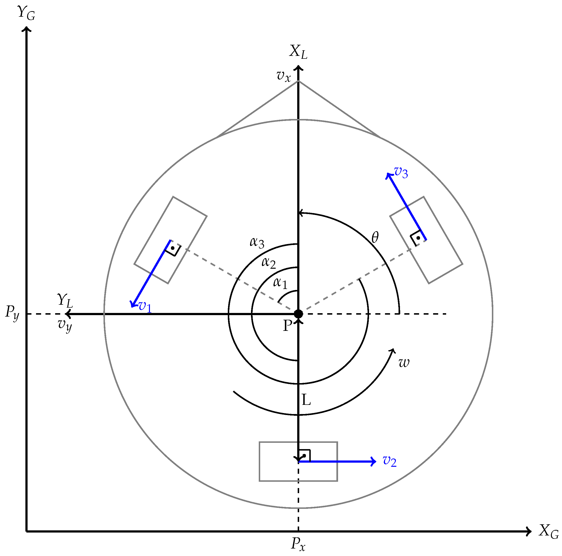
Figure 2 illustrates the Robotino configuration within a global coordinate system ($X_G,Y_G$), which is arbitrarily defined as a fixed reference frame for motion analysis. In addition, a local coordinate system ($X_L,Y_L$) is considered, with its origin at the point $P$, which represents the geometric center of the robot. The orientation of the robot relative to the global system is determined by the angle $\theta$.

Based on kinematic studies of three-wheeled omnidirectional mobile robots in the literature [11,20,21], the kinematic model has been adapted to the specific case of the Robotino version 4. The resulting kinematic equations describe the relationship between the velocities in the global frame ($\dot{x},\dot{y},\dot{\theta }$) and the local frame ($v_x,v_y,\omega$), as well as the relationship between the motion of the robot in its reference frame and the velocities of each individual wheel ($v_1,v_2,v_3$).

In Equation (1), the relationship between the global and local velocities is obtained using the rotation matrix $R\left(\theta \right)$ in Equation (2):

$$\left[\begin{array}{c}\dot{x}\\ \dot{y}\\ \dot{\theta }\end{array}\right]=R\left(\theta \right)\left[\begin{array}{c}{v}_x\\ v_y\\ \omega \end{array}\right]$$

(1)

$$R\left(\theta \right)=\left(\begin{array}{ccc}cos\theta & -sin\theta & 0\\ sin\theta & cos\theta & 0\\ 0& 0& 1\end{array}\right)$$

(2)

To compute the local velocities from the global velocities, the inverse of the rotation matrix is used:

$$\left[\begin{array}{c}\dot{x}\\ \dot{y}\\ \dot{\theta }\end{array}\right]=R\left(\theta \right)\left[\begin{array}{c}{v}_x\\ v_y\\ \omega \end{array}\right]\to \left[\begin{array}{c}{v}_x\\ v_y\\ \omega \end{array}\right]=R{\left(\theta \right)}^{-1}\left[\begin{array}{c}\dot{x}\\ \dot{y}\\ \dot{\theta }\end{array}\right]$$

(3)

$$R{\left(\theta \right)}^{-1}=\left(\begin{array}{ccc}cos\theta & sin\theta & 0\\ -sin\theta & cos\theta & 0\\ 0& 0& 1\end{array}\right)$$

(4)

The relationship between the velocity at the center of the robot and the individual wheel velocities $v_i$ (where $i=1,2,3$) is derived from the geometric arrangement of the omnidirectional wheels. Since these wheels are placed at 120-degree intervals, the velocity of each wheel depends on both the linear and angular motions of the robot, as expressed in Equation (5). This relationship is formulated through the Jacobian matrix J, where ${\alpha }_1$, ${\alpha }_2$, and ${\alpha }_3$ represent the angles between the local coordinate axis $X_L$ and each wheel and L denotes the distance from the center of the robot to each wheel. For the Robotino 4, the wheel angles are defined as ${\alpha }_1={60}^{\circ }$, ${\alpha }_2={180}^{\circ }$, and ${\alpha }_3={300}^{\circ }$, as shown in Equation (6):

$$\left[\begin{array}{c}{v}_1\\ v_2\\ v_3\end{array}\right]=J\left[\begin{array}{c}{v}_x\\ v_y\\ \omega \end{array}\right]$$

(5)

$$J=\left(\begin{array}{ccc}-sin{\alpha }_1& cos{\alpha }_1& L\\ -sin{\alpha }_2& cos{\alpha }_2& L\\ -sin{\alpha }_3& cos{\alpha }_3& L\end{array}\right)=\left(\begin{array}{ccc}-{\displaystyle \frac{\sqrt{3}}{2}}& {\displaystyle \frac{1}{2}}& L\\ 0& -1& L\\ {\displaystyle \frac{\sqrt{3}}{2}}& {\displaystyle \frac{1}{2}}& L\end{array}\right)$$

(6)

Since Robotino DC motors with a permanent magnet [22] are controlled using commands in revolutions per minute (rpm), it is necessary to convert the linear velocities of the wheels into angular velocities, as expressed in Equation (7). In this context, the angular velocities of the motor shafts, denoted by ${\omega }_1$, ${\omega }_2$, and ${\omega }_3$ for each wheel, are considered positive in the counterclockwise direction. Taking into account that the gear reduction ratio is 32:1 (compared with 16:1 in the Robotino 3 [20]) and that the radius of the wheel is r, the relationship between the angular velocity of the motor (in rpm) and the velocity of the wheel is determined by the factor k, as defined in Equation (8):

$$\left[\begin{array}{c}{\omega }_1\\ {\omega }_2\\ {\omega }_3\end{array}\right]=k·J\left[\begin{array}{c}{v}_x\\ v_y\\ \omega \end{array}\right]$$

(7)

$$k={\displaystyle \frac{60s·32}{2\pi ·r}}$$

(8)

The following occurs when determining the local velocities from the wheel velocities:

$$\left[\begin{array}{c}{\omega }_1\\ {\omega }_2\\ {\omega }_3\end{array}\right]=k·J\left[\begin{array}{c}{v}_x\\ v_y\\ \omega \end{array}\right]\to \left[\begin{array}{c}{v}_x\\ v_y\\ \omega \end{array}\right]={\displaystyle \frac{1}{k}}·J^{-1}\left[\begin{array}{c}{\omega }_1\\ {\omega }_2\\ {\omega }_3\end{array}\right]$$

(9)

$$J^{-1}=\left(\begin{array}{ccc}-{\displaystyle \frac{1}{\sqrt{3}}}& 0& {\displaystyle \frac{1}{\sqrt{3}}}\\ {\displaystyle \frac{1}{3}}& -{\displaystyle \frac{2}{3}}& {\displaystyle \frac{1}{3}}\\ {\displaystyle \frac{1}{3L}}& {\displaystyle \frac{1}{3L}}& {\displaystyle \frac{1}{3L}}\end{array}\right)$$

(10)

Once the geometric and kinematic relationships have been established, it is possible to introduce the concept of the motion control strategy.

2.3. Motion Control Strategy

Once the multilayer architecture is presented in Figure 1, this section explains the motion control strategy implemented within the motion control block. The internal structure of this block is illustrated in Figure 3.

As shown in Figure 3, the subsystem follows a structured control pipeline, where a predefined trajectory, such as a lemniscate curve, is generated by the path planning module and is provided as a reference to the Model-based Predictive Control (MPC). The MPC uses this reference ($x_{ref},y_{ref},{\theta }_{ref}$) to compute the optimal velocity commands in the local frame of the robot, considering the kinematic model and the velocity and acceleration constraints of the robot.

The computed velocity commands ($v_{x,ref},v_{y,ref},{\omega }_{ref}$) are then converted into individual wheel speeds (${\omega }_{1,ref},{\omega }_{2,ref},{\omega }_{3,ref}$) using the Jacobian matrix of the robot (J) and the conversion factor k. These references are tracked by a set of PID controllers, which operate at a frequency ten times higher than that of the MPC [22].

After regulation by the PID, the actual angular speeds of the wheels (${\omega }_1,{\omega }_2,{\omega }_3$) are transformed back into local velocity components ($v_x,v_y,\omega$) through the inverse kinematic transformation $v={\displaystyle \frac{1}{k}}·J^{-1}·\omega$. These local velocities are then mapped to the global frame, taking into account the orientation of the robot, to obtain $\dot{x}$, $\dot{y}$, and $\dot{\theta }$. Finally, these global velocity components are integrated over time to obtain the position of the robot ($x,y,\theta$).

A dedicated state estimation block computes the actual position and orientation ($\widehat{x},\widehat{y},\widehat{\theta }$) using data from the wheel encoders and the onboard gyroscope. This estimate is fed back into the MPC, which closes the control loop.

In the following subsection, the structure of the MPC controller is explained in greater detail, focusing on the specific aspects of its implementation.

2.4. Model-Based Predictive Control Approach

Model-based Predictive Control (MPC) is considered the high-level control of Robotino. The MPC controller has the ability to handle system constraints (e.g., physical feasible limits of velocity and acceleration) and optimize control inputs over a prediction horizon.

The goal of MPC in the scheme shown in Figure 3 is to ensure that the system state, as defined by the global coordinates and orientation angle $\mathit{x}\left(k\right)={\left[x\left(k\right)y\left(k\right)\theta \left(k\right)\right]}^T$, follows as close as possible the reference trajectory ${\mathit{x}}_{ref}\left(k\right)$ computed by the path planning module. For this purpose, the MPC controller determines the optimal velocity vector in the local frame (control output $\mathit{u}\left(k\right)={\left[v_x\left(k\right)v_y\left(k\right)\omega \left(k\right)\right]}^T$). The relationship between the control action and system state is obtained by discretizing Equation (1) as

$$\mathit{x}(i+1|k)=\mathit{x}\left(i\right|k)+T_{s}R\left(\theta \left(i\right|k)\right)\mathit{u}\left(i\right|k)$$

(11)

where matrix $R\left(\theta \right(i\left|k\right))$ is the rotation matrix defined in Equation (2). Then, the MPC controller can be defined as the following optimization problem:

$$\begin{array}{c}\underset{\mathit{u}\left(i|k\right)}{min}{\displaystyle \sum _{i=1}^{H_p}}{\left(\mathit{x}\left(i\right|k)-{\mathit{x}}_{ref}\left(k\right)\right)}^{T}Q\left(\mathit{x}\left(i\right|k)-{\mathit{x}}_{ref}\left(k\right)\right)+\mathit{u}{\left(i\right|k)}^{T}P\mathit{u}\left(i\right|k)\hfill \\ \mathrm{s}.\mathrm{t}.\hfill \\ \mathit{x}(i+1|k)=\mathit{x}\left(i\right|k)+T_{s}R\left(\theta \left(i\right|k)\right)\mathit{u}\left(i\right|k)\hfill \\ {\mathit{u}}^{min}\le \mathit{u}\left(i\right|k)\le {\mathit{u}}^{max}\hfill \\ \mathsf{\Delta }{\mathit{u}}^{min}\le \mathsf{\Delta }\mathit{u}\left(i\right|k)\le {\mathsf{\Delta }\mathit{u}}^{max}\hfill \\ {\mathit{x}}^{min}\le \mathit{x}(i+1|k)\le {\mathit{x}}^{max}\hfill \end{array}$$

(12)

where matrices Q and P determine the tracking error and control effort weights in the cost function of the optimization problem. Physical limitations are taken into account, with ${\mathit{u}}^{min}$ and ${\mathit{u}}^{max}$ representing the minimum and maximum velocities and $\mathsf{\Delta }{\mathit{u}}^{min}$ and $\mathsf{\Delta }{\mathit{u}}^{max}$ determining the minimum and maximum accelerations. Finally, ${\mathit{x}}^{min}$ and ${\mathit{x}}^{max}$ define the limits of the robot trajectory.

The optimization problem defined in Equation (12) is a non-linear optimization problem, but with some assumptions, such as a fixed orientation $\theta \left(i\right|k)={\theta }_0\forall i=1,\dots ,H_p$, as proposed in [12], it can be formulated as a quadratic optimization problem. In addition, following the ideas proposed in [14], as the non-linear Equation (11) can be expressed in a Linear Parameter Varying (LPV) form, this allows us to formulate the MPC problem as a quadratic optimization problem, considering a generic trajectory in the three states. The LPV control approach proves successful in research on lateral control in autonomous vehicles [23,24].

2.5. Experimental Validation

Experimental validation of the proposed methodology was performed in several scenarios: laboratory, simulation, and real world.

To ensure that the simulation accurately reflected real-world behavior, an initial laboratory scenario was used to characterize the dynamics of the system and asses the state estimation errors. Based on this foundation, the motion control strategy was validated in the simulation and real-world experiments. The scenarios considered in this section are described below:

• Laboratory scenario—preliminary tests: A series of initial experiments were conducted to characterize the hardware layer and evaluate the accuracy of the onboard sensors (linear encoders and gyroscope) and the state estimation algorithm of the Robotino 4. Since the Robotino 4 platform provides pre-tuned PID parameters, the wheel dynamics under PID control was identified by exciting the system and obtaining the velocity transfer functions. In addition, the quality of the internal state estimation was assessed. These results were used to improve the realism of the simulation model.
• Simulation scenario: This implemented the specific study case shown in Figure 3, which included the path planning layer, the high-level control layer with the MPC, and the low-level control layer with the PID controller. A lemniscate trajectory was selected to test the capability of the controller in tracking the position and orientation of the robot.
• Real-world scenario: Finally, the control architecture was implemented on the physical Robotino 4 platform in the laboratory environment. The same lemniscate trajectory and identical MPC parameters used in the simulation were applied during the real-world experiments to allow for a direct performance comparison.

3. Results

This section presents the simulation and real-world results obtained using the proposed motion control strategy. The following subsections detail the results obtained in each of these scenarios.

3.1. Laboratory Scenario—Preliminary Test

To ensure that the simulation scenario accurately represented the real-world behavior of the system, preliminary laboratory experiments were conducted on the Robotino 4 platform. These experiments focused on two key aspects: the identification of the closed-loop motor dynamics and the tuning of the PID controller, and the evaluation of the state estimation errors.

3.1.1. Identification of Closed-Loop Motor Dynamics

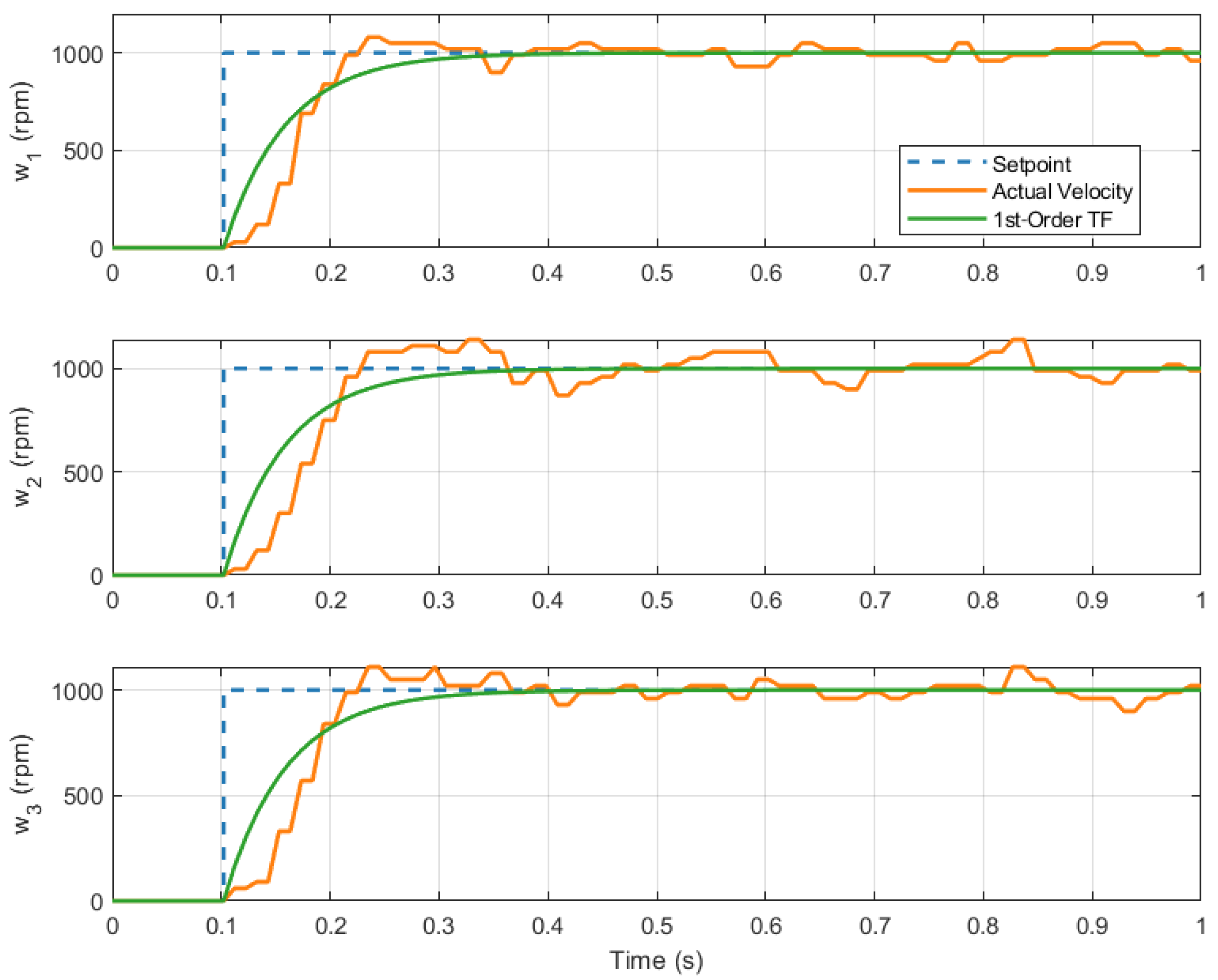
The identification of motor dynamics and PID controllers was performed by applying a set velocity point of 1000 rpm to all three motors simultaneously. The actual wheel velocities were recorded every 10 ms, along with their corresponding timestamps. These data were plotted (Figure 4) and analyzed.

To model the system response, a first-order transfer function was estimated using parameter estimation techniques [25]. The resulting transfer function is given by

$$G\left(s\right)={\displaystyle \frac{K}{\tau s+1}}$$

(13)

where the average time constant for the three wheels was $\tau =0.05$, and the gain K was 1. Figure 4 illustrates the results.

3.1.2. Evaluation of State Estimation Errors

To evaluate the precision of the state estimation, odometry-based localization was compared against the ground-truth measurements obtained through manual tracking. Two open-loop experiments were conducted to quantify the odometry errors under different motion conditions:

• Linear motion test: A constant forward velocity command of $v_x=0.5$ m/s was applied for 10 s. The odometry readings were recorded every 10 ms, and the resulting trajectory is shown in the left graph of Figure 5, alongside the reference trajectory. The real-world measurements confirmed a systematic deviation due to wheel slippage, which was not considered in the odometry. Specifically, the robot exhibited an additional deviation of 5 cm/m along both the X- and Y-axes.
• Rotational motion test: A rotational velocity command of $\omega =0.5$ rad/s was applied for 10 s, and the comparison between the reference and odometry data is shown in the right graph of Figure 5. Although the odometry followed the reference rotation, the real-world measurements revealed a discrepancy between the estimated and actual orientation. The observed deviation was 2 degrees.

The identified motor dynamics model and the quantified state estimation errors were integrated into the simulation scenario to improve the accuracy of the virtual representation of the robot behavior.

3.2. Simulation Scenario

To evaluate the performance of the proposed MPC controller, a simulation scenario was implemented in MATLAB, following the scheme presented in Figure 3. The simulation environment was designed to reflect the spatial constraints of the physical laboratory and the dynamic characteristics of the Robotino, including its maximum velocity and acceleration limits, PIDs, and state estimation errors.

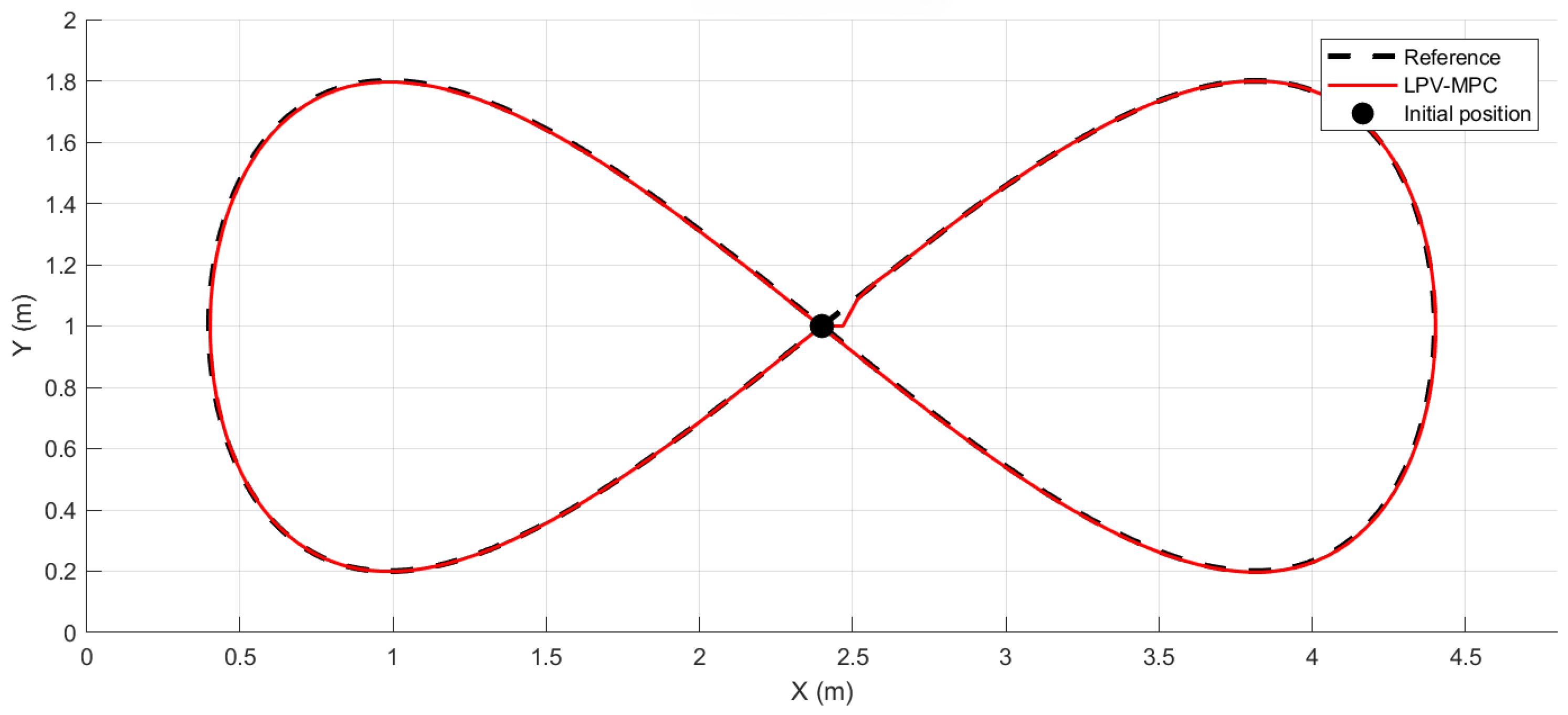
The system was tested using a lemniscate trajectory as a reference trajectory generated by the path planning layer. This trajectory was defined parametrically as

$$\begin{array}{cc}\hfill x_d\left(t\right)& =A_x·sin\left({\displaystyle \frac{2\pi }{T}}·t\right)+c_x\hfill \end{array}$$

(14)

$$\begin{array}{cc}\hfill y_d\left(t\right)& =A_y·sin\left(2·{\displaystyle \frac{2\pi }{T}}·t\right)+c_y\hfill \end{array}$$

(15)

where $T=110$ s was the trajectory period, $A_x=4$ m and $A_y=1.6$ m were the horizontal and vertical amplitudes of the path, and $c_x=2.4$ m and $c_y=1$ m defined the center point of the trajectory center in the workspace.

The optimization problem that implemented the LPV-MPC controller was solved by means of Yalmip [26] and the Gurobi optimization solver. The MPC controller was executed at a sampling time of $0.5$ s, which was 10 times the constant time of the low-level PID control. The following constraints were applied:

• Velocity limits:

  $${\mathit{u}}^{min}=-\left[\begin{array}{c}0.3\mathrm{m}/\mathrm{s}\\ 0.3\mathrm{m}/\mathrm{s}\\ 0.4\mathrm{rad}/\mathrm{s}\end{array}\right],{\mathit{u}}^{max}=\left[\begin{array}{c}0.3\mathrm{m}/\mathrm{s}\\ 0.3\mathrm{m}/\mathrm{s}\\ 0.4\mathrm{rad}/\mathrm{s}\end{array}\right]$$

  (16)
• Acceleration limits:

  $$\mathsf{\Delta }{\mathit{u}}^{min}=-\left[\begin{array}{c}0.15\mathrm{m}/{\mathrm{s}}^2\\ 0.15\mathrm{m}/{\mathrm{s}}^2\\ 0.2\mathrm{rad}/{\mathrm{s}}^2\end{array}\right],\mathsf{\Delta }{\mathit{u}}^{max}=\left[\begin{array}{c}0.15\mathrm{m}/{\mathrm{s}}^2\\ 0.15\mathrm{m}/{\mathrm{s}}^2\\ 0.2\mathrm{rad}/{\mathrm{s}}^2\end{array}\right]$$

  (17)
• Position constraints:

  $${\mathit{x}}^{min}=\left[\begin{array}{c}0\\ 0\end{array}\right]\mathrm{m},{\mathit{x}}^{max}=\left[\begin{array}{c}5\\ 2\end{array}\right]\mathrm{m}$$

  (18)
• Weighting matrices:

  $$Q=\mathrm{diag}(1,1,1),P=\mathrm{diag}(0,0,0)$$

  (19)
• Prediction horizon: $H_p=5$.
• Initial state: ${\mathit{x}}_0={\left[\begin{array}{ccc}2.4\mathrm{m}& 1\mathrm{m}& 0\mathrm{rad}\end{array}\right]}^{\prime }$.

To model the motor dynamics and the effect of the low-level control loop, a first-order transfer function identified from the experimental data (see Section 3.1.1) was integrated into the simulation. The transfer function was evaluated with a sampling time of $0.05\mathrm{s}$, which matched the execution frequency of the on-board PID controllers. At each MPC update (every $0.5\mathrm{s}$), the optimal velocity commands were mapped to wheel velocities and applied as reference inputs to the motor dynamic. During each MPC interval, the wheel velocities were propagated using the motor transfer function, and the actual velocities applied to the system were calculated as the average wheel velocity over the interval.

In addition, state estimation errors were introduced into the simulation to better approximate real-world conditions. At each sampling step, a constant positive error (quantified in Section 3.1.2) was added to the state: $0.05$ m in both the x- and y-positions and 2 degrees to the orientation $\theta$.

To evaluate the performance of the reference tracking, the mean squared error (MSE) was calculated for each state variable. The values obtained are shown in

Table 2. Mean squared error for each state.

State Variable	MSE Value
x (m)	$6.1161\times {10}^{-5}$
y (m)	$5.5428\times {10}^{-5}$
$\theta$ (rad)	$1.1667\times {10}^{-6}$

.

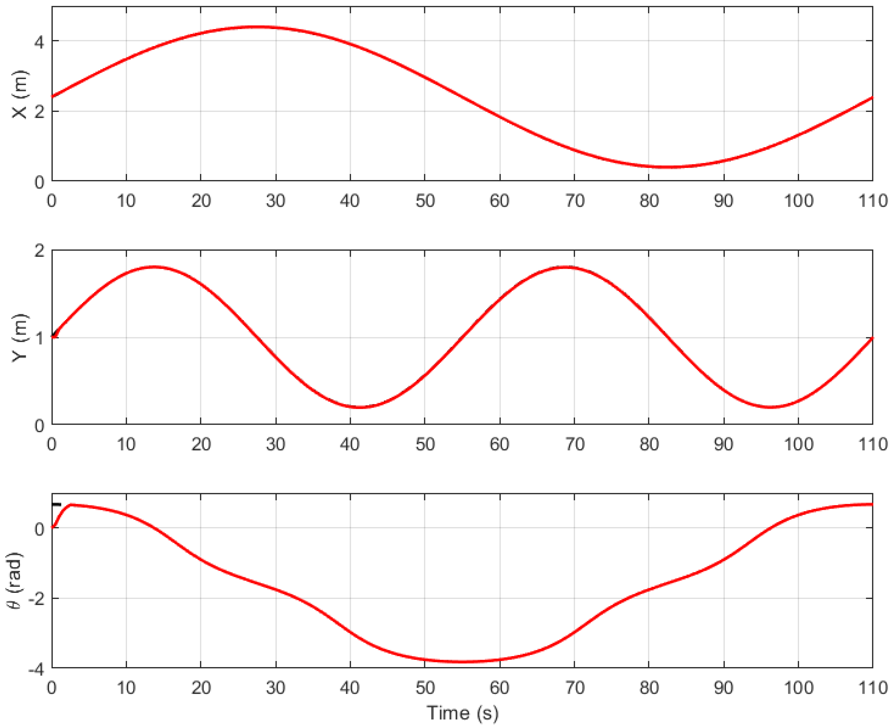
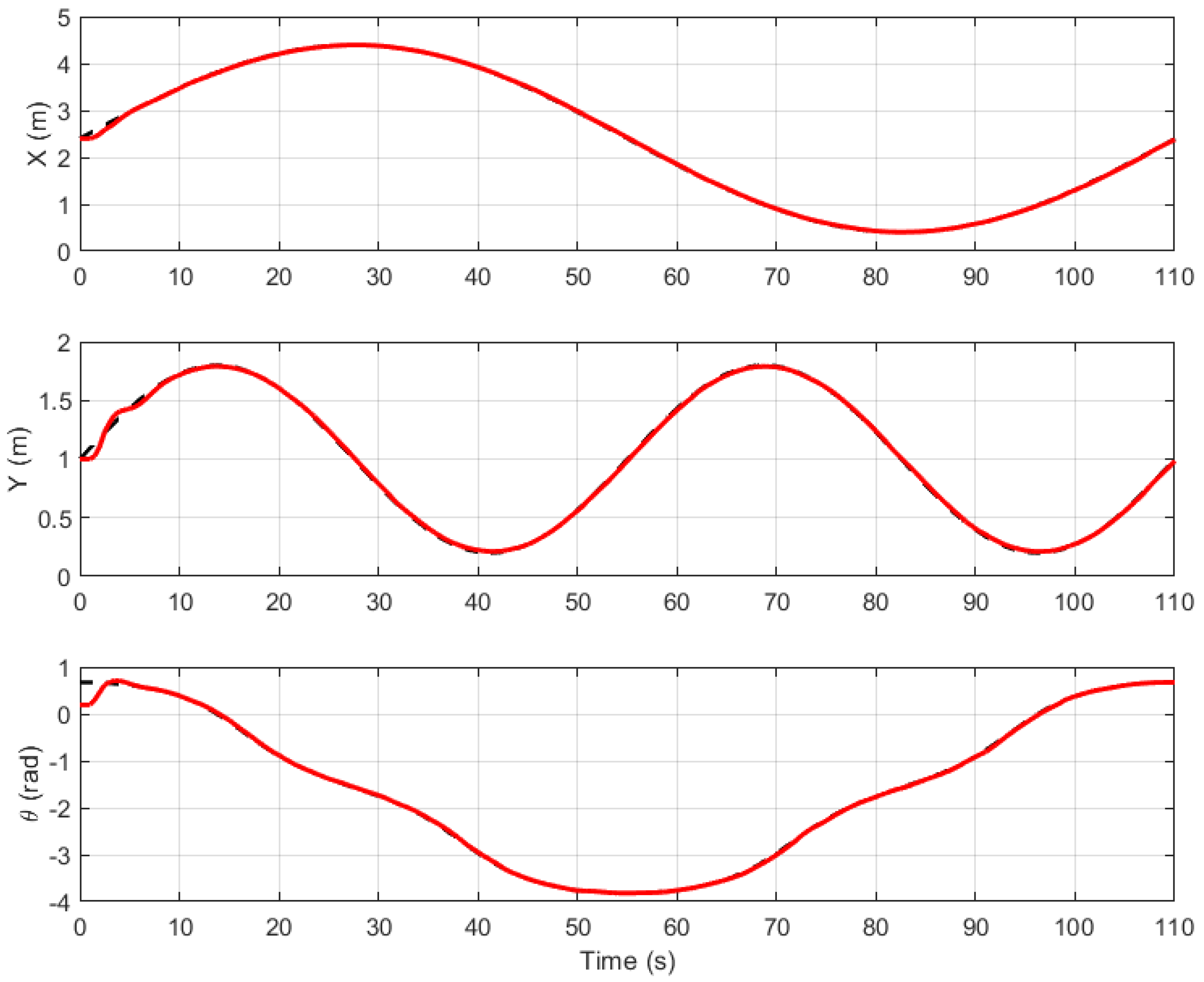
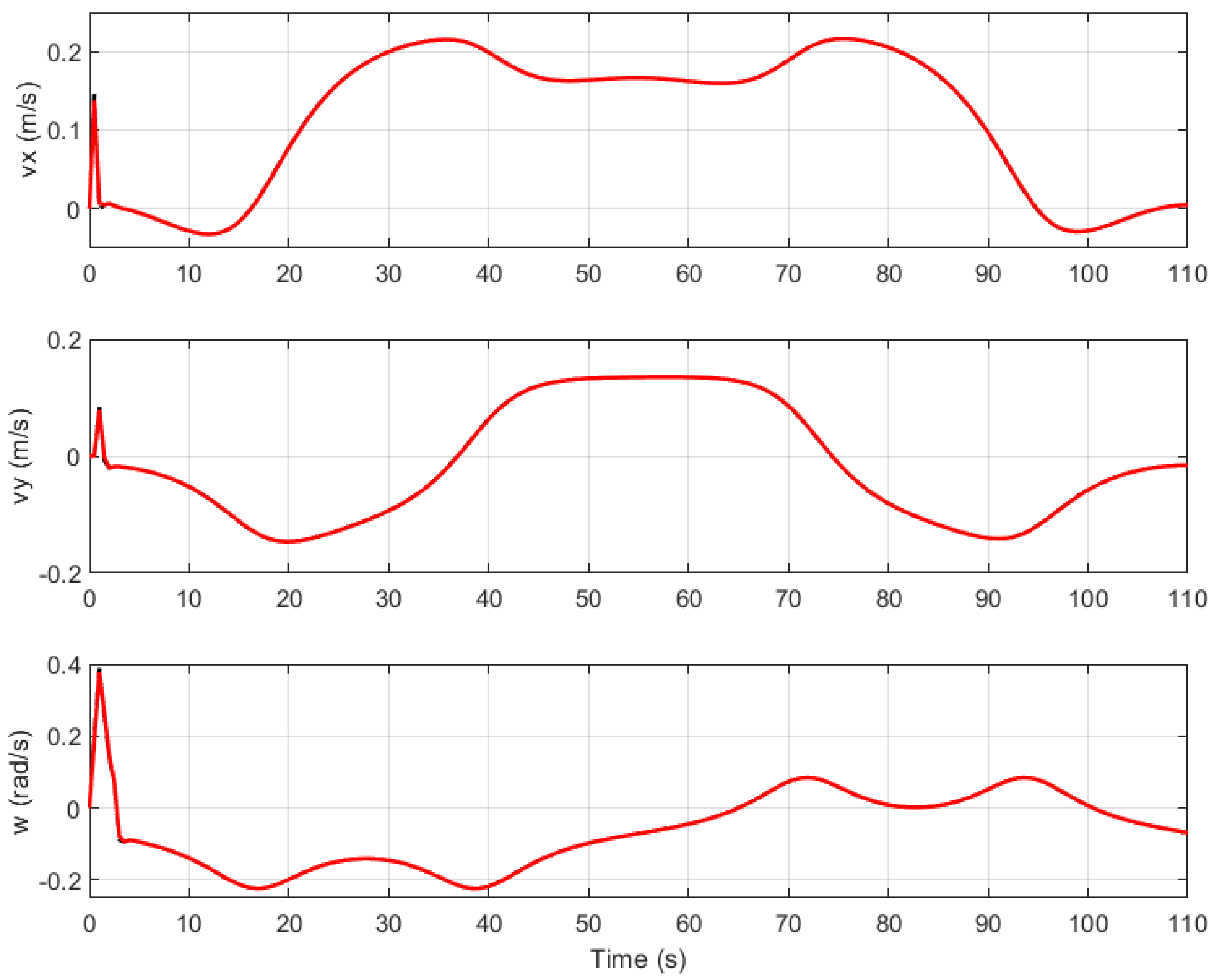
The following figures illustrate different aspects of the simulation results. Figure 6 shows the overall trajectory tracking, comparing the reference path with the trajectory followed by the robot. Figure 7 provides a time-based comparison of the position and orientation states of the robot (x, y, and $\theta$). Figure 8 compares the local reference velocities ($v_x$, $v_y$, $\omega$) with the actual velocities applied. 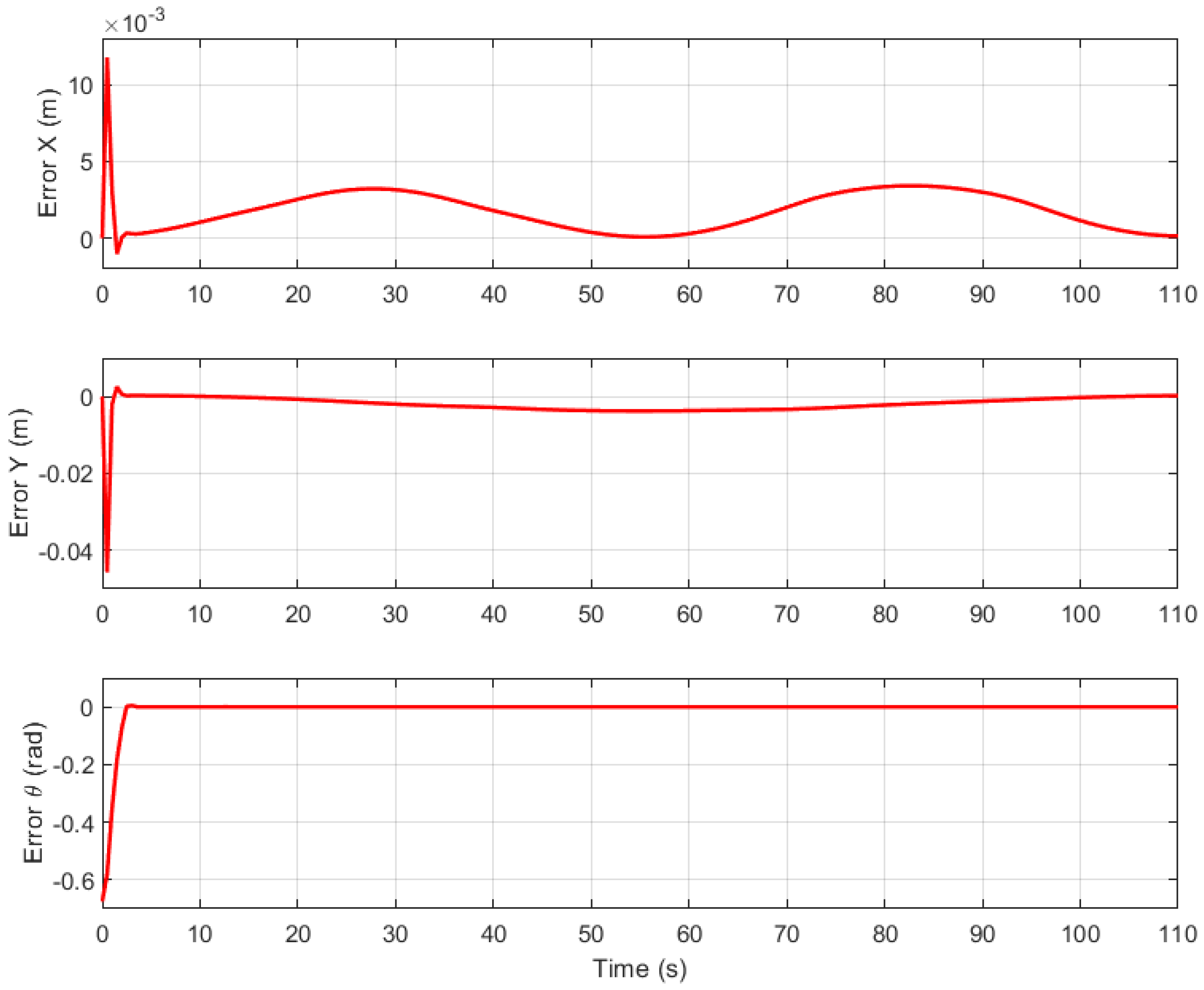Figure 9 evaluates the actuator performance by comparing the reference and actual wheel velocities applied to each of the three wheels, and Figure 10 presents the evolution of tracking errors in x, y, and $\theta$.

3.3. Real-World Scenario

After completing the simulation scenario, the motion control strategy was implemented on the physical Robotino 4 platform to evaluate its real-world performance. In this scenario, the same lemniscate trajectory, controller parameters, and MPC configuration used in the simulation were applied to enable a direct comparison between the simulated and real-world performances.

The state estimation in the real-world setup relied on the on-board algorithms provided by the manufacturer, which fuse data from a gyroscope and incremental encoders mounted on each wheel. These estimations serve as feedback states for the controller.

The real-time control loop was executed on a laptop that ran the MPC algorithms. Communication with the robot was established via a wired Ethernet/IP connection using the TCP protocol, which ensured fast and reliable data transmission to maintain real-time operation. The laptop sent local velocity commands ($v_x$, $v_y$, $\omega$) to the robot and received odometry data estimated by the manufacturing on-board algorithms.

To achieve reliable timing and low-latency communication, a multithreaded C++ interface was implemented using the API provided by the manufacturer. This interface handled the sending commands and receiving odometry data continuously during the execution of the trajectory.

During the initial testing, two problems were identified. The first issue involved the gyroscope measurement convention. The on-board system reported the orientation of the robot within the interval $[-\pi ,\pi ]$, where 0 corresponded to the forward direction of the robot. As the robot rotated, its angular reading would suddenly jump from $\pi$ to $-\pi$ (or vice versa), creating discontinuities in the orientation signal.

These discontinuities interfered with the calculation of orientation tracking errors, which led to inaccurate control inputs. To address this, a compensation mechanism was implemented in the control system to track the cumulative rotation of the robot. This correction ensured a continuous, unwrapped orientation signal that faithfully represented the robot heading throughout the trajectory, which eliminated artificial jumps at the $\pm \pi$ boundary.

The second issue identified during the first experiment was related to the oscillatory behavior in the robot movement. This was caused by the lack of penalization in the control input in the MPC cost function (the weighting matrix $P=0$). As a result, the controller produced unnecessarily aggressive commands. In the final test, this was corrected by setting $P=diag(1,1,1)$, which resulted in a smoother response that was more consistent with the simulated behavior.

To quantify the performance, the mean squared error (MSE) was calculated for each state variable. The results are shown in

Table 3. Real-world mean squared error for each state.

State Variable	MSE Value
x (m)	$3.1358\times {10}^{-4}$
y (m)	$2.0319\times {10}^{-4}$
$\theta$ (rad)	$1.6000\times {10}^{-3}$

.

The following figures illustrate the tracking performance of the real-world experiment following the lemniscate trajectory. Figure 11 shows the overall path tracking and compares the desired trajectory with the one executed by the robot. Figure 12 presents the time-based tracking of position (x, y) and orientation ($\theta$). Figure 13 shows the evolution of the tracking errors in x, y, and $\theta$.

4. Discussion

Regarding the high-level control layer of the multilayer architecture, the use of MPC presents several advantages to control the Robotino. First, the physical limitations on velocities and accelerations can be explicitly incorporated into the controller as constraints within the optimization problem. Second, obstacles (whether predefined during path planning or detected online) can be handled as additional constraints. Moreover, model inaccuracies, such as state estimation errors or nonlinear approximations, can be addressed by introducing uncertainties, enabling the use of robust control strategies. These capabilities are considerably more challenging, or even infeasible, to achieve using classical methods, like LQR or adaptive control, which struggle to effectively handle hard constraints. Finally, due to the relatively simple kinematics of the Robotino, the computational complexity of the MPC problem is significantly lower than in more demanding systems, such as multi-joint robotic arms [27], making real-time implementation more practical.

The adoption of LPV formulation facilitates an efficient implementation of the original MPC strategy. By linearizing the system dynamics at each sampling instant, the controller achieves a good balance between computational cost and control accuracy. This approach proves particularly advantageous for real-time embedded applications where processing resources are constrained.

The results obtained in both simulation and real-world scenarios show that the robot followed the reference trajectory with minimal error. The largest deviation occurred at the beginning of the motion due to acceleration constraints, as the robot started from a stationary state. However, this initial error rapidly decreased and the tracking error became negligible as the trajectory evolved.

A key decision that improved the real-world performance of the robot was the modification of the penalty matrix P in the controller cost function. Initially, setting $P=0$ meant that variations in control inputs were not penalized, which resulted in overly aggressive commands and oscillatory behavior during trajectory tracking. This configuration is common in cases where the control inputs were unconstrained in magnitude. By updating the penalty to $P=\mathrm{diag}(1,1,1)$, a balanced penalization was introduced for the three control variables, which led to smoother and more stable robot behavior.

The comparison between the simulation and the experimental results shows that the most noticeable difference appears during the transient phase of the motion. In this regime, the real-world experiment shows slightly larger tracking errors compared to the simulation. This is primarily due to physical effects such as mass, inertia, and acceleration saturation, which have a stronger impact in real conditions. While simulations are conducted under idealized conditions with perfectly known parameters, the real environment introduces unmodeled factors like friction, mechanical wear, and structural nonlinearities. These effects are especially noticeable at the start of the motion. Nevertheless, in both cases the robot successfully followed the lemniscate trajectory, with correct wheel behavior and no significant slippage [28].

5. Conclusions

This paper presents the design and evaluation of an MPC strategy integrated into a multilayer architecture for a three-wheeled omnidirectional mobile robot. The proposed methodology is based on the modular design of each control layer, followed by step-by-step integration and validation prior to deployment on the real platform. This study focused on the Motion Control layer, which serves as the core of the architecture.

The performance of the proposed motion control strategy was validated in MATLAB simulations and a real-world scenario using a lemniscate trajectory as a reference. The simulation incorporated motor dynamics and state estimation errors, which ensured a closer approximation to real-world conditions. The results demonstrated that the proposed LPV-MPC controller was capable of tracking the desired trajectory (robot position and orientation) in both the simulation and real-world scenarios.

In terms of the orientation control, the proposed LPV-MPC framework enables the robot to track time-varying references in $\theta$, a significant advantage over conventional methods that often assume a fixed or quasi-static heading [11]. This capability is especially valuable in applications that require precise and dynamic orientation adjustments, such as visual-based navigation, docking, or object manipulation.

Future work will focus on expanding the remaining layers of the proposed multilayer architecture, particularly the obstacle avoidance, fault tolerance strategy, and fault diagnosis modules. For obstacle avoidance, the integration of proximity sensors will enable the detection of nearby objects. Initially, this functionality may involve stopping the robot, but further development will focus on trajectory replanning to allow for continuous navigation around obstacles without halting [29].

In the context of fault tolerance, particular emphasis will be placed on handling actuator faults, especially motor failures. The LPV-MPC controller will be reconfigurable in real time by updating the model and/or constraints within the optimization problem. This will enable the robot to continue its task autonomously or, in cases of critical failure, to delegate the mission to another robot.

Furthermore, future developments will consider the incorporation of model uncertainties, such as state estimation errors or unmodeled dynamics, within the MPC framework to improve the robustness in real-world deployments.

Finally, future work will involve transitioning the current MATLAB framework to more versatile programming environments, such as Python and C++, with the aim of deploying the full system in ROS 2 and Gazebo. As part of this transition, the need to reduce the execution time of the algorithms will be assessed. Therefore, the goal will be to provide guidelines to determine which controller can be the best candidate for its final implementation on robot hardware. The purpose of this integration is to anticipate the detection of potential problems in the design phase rather than encountering them during the implementation phase in autonomous navigation, where a serious anomaly in the behavior of the robot could be irreversible.