Enhancing Visual–Inertial Odometry Robustness and Accuracy in Challenging Environments

Abstract

Visual–Inertial Odometry (VIO) algorithms are widely adopted for autonomous drone navigation in GNSS-denied environments. However, conventional monocular and stereo VIO setups often lack robustness under challenging environmental conditions or during aggressive maneuvers, due to the sensitivity of visual information to lighting, texture, and motion blur. In this work, we enhance an existing open-source VIO algorithm to improve both the robustness and accuracy of the pose estimation. First, we integrate an IMU-based motion prediction module to improve feature tracking across frames, particularly during high-speed movements. Second, we extend the algorithm to support a multi-camera setup, which significantly improves tracking performance in low-texture environments. Finally, to reduce the computational complexity, we introduce an adaptive feature selection strategy that dynamically adjusts the detection thresholds according to the number of detected features. Experimental results validate the proposed approaches, demonstrating notable improvements in both accuracy and robustness across a range of challenging scenarios.

1. Introduction

Visual–Inertial Odometry (VIO) is a widely used navigation solution for robotics, particularly in GPS-denied environments [1,2]. Processing IMU and image data, it is able to provide real-time position estimation in previously unknown environments. While LiDAR-based SLAM algorithms generally outperform VIO in terms of accuracy and robustness in structured, feature-rich environments [3,4], VIO remains advantageous in scenarios where LiDAR is ineffective, such as large open spaces with few detectable features [5]. Additionally, VIO is particularly well suited for drones due to the lower weight and occupied space of cameras compared to LiDAR sensors [6,7]. It is worth noting that drones are typically equipped with cameras to collect visual information of the environment. Therefore, utilizing these cameras for both perception and localization optimizes onboard resource usage, enhancing overall system efficiency.

Despite its advantages, VIO suffers from inherent limitations, such as drift accumulation over time due to errors in IMU integration and inaccuracies in 3D feature tracking. Furthermore, motion blur during high-speed maneuvers and the presence of featureless environments can severely degrade tracking quality, potentially leading to failures in navigation. A notable example of VIO’s vulnerability occurred with NASA’s Ingenuity helicopter, which operated on Mars as part of the Mars 2020 mission. Ingenuity relied on a VIO system using a downward-facing monocular grayscale camera. On 18th January 2024, its last flight resulted in a crash causing damages in the blades and making the drone unable to fly again. NASA’s subsequent investigation confirmed that the featureless terrain was responsible for the crash [8]. This incident highlights the importance of enhancing VIO algorithms to ensure robustness in featureless environments. Over the past two decades, several VIO algorithms have been developed to improve localization accuracy and robustness. Non-Linear Factor Recovey (NFR), proposed in [9], has emerged as one of the most valuable solutions for visual–inertial mapping. This methodology is implemented in the open-source Basalt project (https://github.com/VladyslavUsenko/basalt, accessed on 22 May 2025). This VIO algorithm achieves state-of-the-art performance on benchmark datasets. Its main novelty lies in leveraging non-linear factors extracted from previous keyframes, which are subsequently used in the global bundle adjustment. In this work, we propose improvements to the Basalt project aimed at increasing its robustness, particularly in high-speed motion scenarios and featureless environments. Our contributions are summarized as follows:

• IMU-based Feature Prediction: We introduce a method for predicting feature positions in the next frame using IMU data. Instead of assuming that features remain at the same pixel across consecutive frames, our approach integrates IMU measurements to estimate feature displacement, starting from the last VIO-predicted position. This method improves tracking accuracy during rapid movements. Details are provided in Section 3.1.
• Multi-Camera Extension for Featureless Environments: To mitigate VIO failures in featureless scenarios, we extend Basalt to support a multi-camera setup. By increasing the field of view, this approach significantly reduces the possibility of encountering textureless regions that may lead the algorithm to fail. Implementation details are discussed in Section 3.2.
• Adaptive Threshold for Feature Extraction: Since the multi-camera setup results in a considerable increase in computational complexity, we propose a dynamic feature detection strategy to mitigate the computational load. Specifically, we introduce an adaptive thresholding mechanism that adjusts feature detection parameters. The implementation of this optimization is detailed in Section 3.3.

Due to its high positional accuracy and efficient CPU usage, the open-source Basalt algorithm has been improved and adapted in two other open-source projects. In [10], the authors modify Basalt for a monocular setup, introducing a novel method for evaluating the scale factor to locate the feature in the 3D space. The “Basalt for Monado” project (https://gitlab.freedesktop.org/mateosss/basalt, accessed on 22 May 2025) integrates Basalt with Monado (https://gitlab.freedesktop.org/monado/monado, accessed on 22 May 2025), enhancing the tracking for XR devices and extending it to support multi-camera setups. However, to the best of our knowledge, no official documentation or published research papers describe this multi-camera implementation. With the goal of improving the robustness of VIO algorithms, several solutions have been proposed in the last decades. In [11], the authors propose a VIO algorithm based on line features. Their contribution consists of the reduction of the influence of lines upon dynamic objects on system robustness merging the results coming from the semantic segmentation, optical flow, and re-projection error. Then, a weight-based method adjusts the line features matrix in the optimization process. The work in [12] proposes a methodology to enhance the performances of a VIO algorithm encountering different brightness conditions. The methodology couples a model-based Left Invariant Extended Kalman Filter (LIEKF) with a statistical neural network, both driven by raw inertial measurement. While these approaches mitigate common failures of VIO algorithms, textureless environments continue to pose a significant challenge. Due to its capability to capture images by multiple perspectives, a multi-camera setup remains one of the most effective and widely adopted solutions to detect features in textureless environments.

The approach in [13] presents an implementation of a multi-camera setup, where two stereo cameras face opposite directions. The authors demonstrate its superiority over state-of-the-art VIO algorithms. However, since the paper was published in 2007, it relies on an Extended Kalman Filter (EKF) for pose estimation rather than modern optimization techniques such as bundle adjustment or Factor Graphs, which are widely used today. In [14], a generalized multi-camera approach is introduced. The work supports an arbitrary number of cameras in various configurations (overlapping and non-overlapping fields of view). This implementation is based on [15], one of the first versions of the well-known open-source SLAM algorithm. Similarly, [16] proposes an alternative multi-camera approach and compares it with [14], proving its superiority on custom datasets. The paper [17] presents another multi-camera setup, consisting of a stereo camera with two additional monocular cameras mounted on the sides. To optimize computational efficiency and performance, the authors track features from the stereo camera across the mono cameras, leveraging the shared field of view. Another approach [18] focuses specifically on configurations where camera fields of view do not overlap. Additionally, the article available at [19] details an implementation tailored for UAVs. While the proposed method supports an arbitrary number of cameras, the authors provide results only for a dual-camera setup. To the best of our knowledge, no existing research extends Basalt to a multi-camera setup. Moreover, none of the previous works have been explicitly tested on UAVs. A key challenge in deploying multi-camera systems on drones is the computational load. Since UAVs must allocate processing power to other demanding tasks such as image processing and perception algorithms, computationally intensive processes such as VIO algorithms must be optimized to maintain a bounded computational load. Previous studies do not address CPU consumption. The paper [20] analyzes computational load in a multi-camera setup, comparing the proposed algorithm to ORB-SLAM 3 ([21]), including CPU usage. However, reported CPU loads are never above 300% for more than two cameras. This makes the algorithm impractical for many onboard computers commonly used in autonomous drones, such as Jetson platforms. In [22], the authors propose an implementation of a multi-camera setup with non-overlapping images. Even if the paper provides CPU load considerations, the performances are evaluated without tracking features across the cameras. While this approach accomplishes a reduction in the CPU load, it omits the feature triangulation in the current frame, compromising the accuracy of the 3D landmarks’ estimated position. In this paper, we propose improvements to the Basalt algorithm, specifically aimed at enhancing UAV localization. To enable the extension of Basalt to a multi-camera setup while ensuring feasibility on resource-constrained UAV platforms, we introduce a methodology for reducing computational load.

2. Nomenclature

In this section, we define all the symbols used in the paper. Table 1 contains all the definitions.

Table 1. Nomenclature of all used symbols.

Symbol	Definition
Subindex W	Inertial reference system
Subindex C	Camera reference system
${\mathit{\omega }}_{WC}$	Measured angular velocity of the camera frame C with respect to the inertial frame W
${\tilde{\mathit{\omega }}}_{WC}$	True angular velocity of the camera frame C with respect to the inertial frame W
${\mathbf{a}}_{WC}$	Measured linear acceleration of the camera frame C with respect to the inertial frame W
${\tilde{\mathbf{a}}}_{WC}$	True linear acceleration of the camera frame C with respect to the inertial frame
${\mathbf{b}}_g$	Gyroscope bias
${\mathbf{b}}_a$	Accelerometer bias
${\mathit{\eta }}_g$	Gyroscope noise
${\mathit{\eta }}_a$	Accelerometer noise
${\mathbf{R}}_{WC}$	The 3 × 3 rotation matrix expressing the rotation from the camera frame C to the inertial frame W
$\mathbf{g}$	Gravity acceleration in the inertial reference frame W
×	Skew-matrix operator 1
exp	Exponential map 2
${\mathbf{p}}_{\mathbf{WC}}$	Position of the camera C in the inertial frame W
${\mathbf{v}}_{\mathbf{WC}}$	Velocity of the camera C in the inertial frame W
$\Delta t$	Time interval between two consecutive IMU measurements
$t_k$	Time step at a discrete time k
${\mathbf{T}}_{C_{k-1}{C}_k}$	The 4 × 4 transformation matrix expressing the transformation from the camera C frame in the k step to the $k-1$ step
${\mathbf{T}}_{WC}$	The 4 × 4 transformation matrix expressing the transformation from the camera C to the inertial frame W
${\mathbf{p}}_f$	3D position of one feature in the inertial frame W
${\mathbf{p}}_f^{hom}$	3D position of one feature in homogeneous coordinates
$\tilde{z}$	Average depth of the triangulated landmarks
$tracked\_feature$	Number of tracked features
$min\_feature$	Minimum number of tracked features that guarantee robustness in pose estimation
r	Ratio between $tracked\_feature$ and $min\_feature$
e	Base of natural logarithm and exponential function
k	Feature gain
$\tau$	Scale factor for feature detection threshold

¹ Given a vector $\mathit{\omega }=\left[\begin{array}{c}{\omega }_x\\ {\omega }_y\\ {\omega }_z\end{array}\right]$, its skew-symmetric matrix ${\mathit{\omega }}^{\times }\in {\mathbb{R}}^{3\times 3}$ is defined as ${\mathit{\omega }}^{\times }=\left[\begin{array}{ccc}0& -{\omega }_z& {\omega }_y\\ {\omega }_z& 0& -{\omega }_x\\ -{\omega }_y& {\omega }_x& 0\end{array}\right].$ ² The rigorous definition of this operator can be found in [23].

Table 1. Nomenclature of all used symbols.

Symbol	Definition
Subindex W	Inertial reference system
Subindex C	Camera reference system
${\mathit{\omega }}_{WC}$	Measured angular velocity of the camera frame C with respect to the inertial frame W
${\tilde{\mathit{\omega }}}_{WC}$	True angular velocity of the camera frame C with respect to the inertial frame W
${\mathbf{a}}_{WC}$	Measured linear acceleration of the camera frame C with respect to the inertial frame W
${\tilde{\mathbf{a}}}_{WC}$	True linear acceleration of the camera frame C with respect to the inertial frame
${\mathbf{b}}_g$	Gyroscope bias
${\mathbf{b}}_a$	Accelerometer bias
${\mathit{\eta }}_g$	Gyroscope noise
${\mathit{\eta }}_a$	Accelerometer noise
${\mathbf{R}}_{WC}$	The 3 × 3 rotation matrix expressing the rotation from the camera frame C to the inertial frame W
$\mathbf{g}$	Gravity acceleration in the inertial reference frame W
×	Skew-matrix operator 1
exp	Exponential map 2
${\mathbf{p}}_{\mathbf{WC}}$	Position of the camera C in the inertial frame W
${\mathbf{v}}_{\mathbf{WC}}$	Velocity of the camera C in the inertial frame W
$\Delta t$	Time interval between two consecutive IMU measurements
$t_k$	Time step at a discrete time k
${\mathbf{T}}_{C_{k-1}{C}_k}$	The 4 × 4 transformation matrix expressing the transformation from the camera C frame in the k step to the $k-1$ step
${\mathbf{T}}_{WC}$	The 4 × 4 transformation matrix expressing the transformation from the camera C to the inertial frame W
${\mathbf{p}}_f$	3D position of one feature in the inertial frame W
${\mathbf{p}}_f^{hom}$	3D position of one feature in homogeneous coordinates
$\tilde{z}$	Average depth of the triangulated landmarks
$tracked\_feature$	Number of tracked features
$min\_feature$	Minimum number of tracked features that guarantee robustness in pose estimation
r	Ratio between $tracked\_feature$ and $min\_feature$
e	Base of natural logarithm and exponential function
k	Feature gain
$\tau$	Scale factor for feature detection threshold

¹ Given a vector $\mathit{\omega }=\left[\begin{array}{c}{\omega }_x\\ {\omega }_y\\ {\omega }_z\end{array}\right]$, its skew-symmetric matrix ${\mathit{\omega }}^{\times }\in {\mathbb{R}}^{3\times 3}$ is defined as ${\mathit{\omega }}^{\times }=\left[\begin{array}{ccc}0& -{\omega }_z& {\omega }_y\\ {\omega }_z& 0& -{\omega }_x\\ -{\omega }_y& {\omega }_x& 0\end{array}\right].$ ² The rigorous definition of this operator can be found in [23].

3. Materials and Methods

3.1. IMU-Based Feature Prediction

To track a feature from one frame to another, Basalt employs a frame-to-frame approach. For each camera, the features from the previous frame are tracked by searching for similar patterns in the image using the Lucas–Kanade method. The accuracy of this tracking depends heavily on the initial choice of the feature’s pixel position in the previous frame. Basalt’s original implementation initializes the position of the feature based on its location in the previous frame, assuming that the feature’s position hasn’t changed significantly between frames and that no motion blur has occurred. This assumption works well when the camera motion is slow and the scene remains relatively stable. However, when rapid movements occur, the feature’s position can change drastically between frames, making it challenging to track it accurately. In such cases, the algorithm may fail to track features reliably, which can compromise the accuracy of the estimated trajectory. This is especially problematic in drone applications, where fast movements and rapid changes in orientation are common. In these scenarios, having a method to estimate the feature positions without being constrained by the actual frame-to-frame motion could significantly improve the robustness of the tracking.

To mitigate the impact of the motion blur introduced by rapid movements, we integrate in Basalt a methodology that leverages IMU data to predict the feature positions before a new camera frame is available. The approach begins by estimating the last position of the camera based on the VIO algorithm and then uses the IMU data to predict the camera’s position in the next frame. As soon as the new frame arrives, the relative transformation between the previously estimated camera position and the actual position is calculated. This transformation is then used to estimate the feature positions in the new frame, accounting for the extrinsic calibration parameters of each camera.

Relying on IMU data makes the tracking of features more resilient to fast movements, ensuring a more accurate and robust estimation of the trajectory even under challenging conditions such as rapid drone motion. This methodology helps to improve the overall performance of the VIO system, making it more reliable for real-time applications where high-speed motion is common.

As shown in [23], given the reference system of the camera (C), and an inertial reference system (W), the angular velocity ${\tilde{\mathit{\omega }}}_{WC}$ and the acceleration ${\tilde{\mathbf{a}}}_{WC}$ of the camera C with respect to the reference system W are

$${\tilde{\mathit{\omega }}}_{WC}\left(t\right)={\mathit{\omega }}_{WC}\left(t\right)+{\mathbf{b}}_{\mathbf{g}}\left(t\right)+{\mathit{\eta }}_g\left(t\right)$$

(1)

$${\tilde{\mathbf{a}}}_{WC}\left(t\right)={\mathbf{a}}_{WC}\left(t\right)+{\mathbf{R}}_{WC}\left(t\right)\mathbf{g}+{\mathbf{b}}_{\mathbf{a}}\left(t\right)+{\mathit{\eta }}_a\left(t\right)$$

(2)

where

• ${\mathit{\omega }}_{WC}$ is the true angular velocity of the camera estimated by the IMU;
• ${\mathbf{b}}_g$ is the gyroscope bias;
• ${\mathbf{b}}_a$ is the accelerometer bias;
• ${\mathit{\eta }}_g$ is the gyroscope noise;
• ${\mathit{\eta }}_a$ is the accelerometer noise;
• ${\mathbf{R}}_{WC}$ is the rotation of the camera frame with respect to the inertial frame;
• $\mathbf{g}$ is the gravity acceleration in the inertial reference system.

The derivative of the rotation of the camera frame with respect to the inertial frame can be evaluated by

$${\dot{\mathbf{R}}}_{WC}\left(t\right)={\mathbf{R}}_{WC}\left(t\right){[{\tilde{\mathit{\omega }}}_{WC}\left(t\right)-{\mathbf{b}}_{\mathbf{g}}\left(t\right)-{\mathit{\eta }}_g\left(t\right)]}^{\times }$$

(3)

where ^× is the skew-matrix operator (see Table 1). Integrating (3), we obtain the rotation of the camera in the next time step:

$${\mathbf{R}}_{WC}\left(t_{k+1}\right)={\mathbf{R}}_{WC}\left(t_k\right)exp({[{\tilde{\mathit{\omega }}}_{WC}\left(t_k\right)-{\mathbf{b}}_{\mathbf{g}}\left(t_k\right)-{\mathit{\eta }}_g\left(t_k\right)]}^{\times }\Delta t)$$

(4)

where the operator $exp\left(\right)$ is the exponential matrix operator (see Table 1). Integrating two times (2), we can obtain the position of the camera in the inertial reference system ${\mathbf{p}}_{WC}$ in the next time step:

$${\mathbf{p}}_{WC}\left(t_{k+1}\right)={\mathbf{p}}_{WC}\left(t_k\right)+{\mathbf{v}}_{WC}\left(t_k\right)\Delta t+{\displaystyle \frac{1}{2}}\left(({\mathbf{a}}_{WC}-{\mathbf{R}}_{WC}\left(t_k\right){\mathbf{b}}_a)+\mathbf{g}\right)\Delta t^2$$

(5)

where ${\mathbf{v}}_{WC}$ is the velocity of the camera with respect to the inertial reference system.

Equations (4) and (5) can be used to predict the position of the camera in the current frame at $t_k$. The transformation matrix ${\mathbf{T}}_{C_{k-1}{C}_k}$ between the camera from the current frame to the previous frame is

$${\mathbf{T}}_{C_{k-1}{C}_k}={\mathbf{T}}_{WC}{\left(t_k\right)}^{-1}{\mathbf{T}}_{WC}\left(t_{k-1}\right)$$

(6)

where

$${\mathbf{T}}_{WC}\left(t\right)=\left[\begin{array}{cc}{\mathbf{R}}_{WC}\left(t\right)& {\mathbf{p}}_{WC}\left(t\right)\\ 0& 1\end{array}\right]$$

(7)

Now, we unproject each feature to obtain the homogeneous coordinates ${\mathbf{p}}_f^{hom}$ and rescale them by the average depth evaluated in the previous step to obtain the 3D position of the feature ${\mathbf{p}}_f$:

$${\mathbf{p}}_f\left(t_{k-1}\right)={\mathbf{p}}_f^{hom}\left(t_{k-1}\right)\ast \tilde{z}$$

(8)

where $\tilde{z}$ is the average depth of the landmark collected in the previous steps. Note that the feature position refers to the previous time step $t_{k-1}$. Knowing the 3D position of each feature in the previous time step $t_{k-1}$, we can predict their 3D position at the current frame $t_k$:

$${\mathbf{p}}_f\left(t_k\right)={\mathbf{T}}_{C_{k-1}{C}_k}^{-1}{\mathbf{p}}_f\left(t_{k-1}\right)$$

(9)

Then, we can project the 3D feature in the image plane knowing the intrinsic calibration parameters of the camera to estimate the positions of the features in the current frame.

3.2. Multi-Camera Setup

A multi-camera setup enhances a VIO algorithm in two ways:

• It increases the field of view, allowing for the tracking of more features across frames.
• It improves the 3D position estimation of landmarks, as more observations of the same landmark are made from different baselines.

To generalize Basalt for a multi-camera setup, we extend the optical flow generation process to accommodate an arbitrary number of cameras. We detail our methodology for tracking features across images when portions of the field of view are shared between multiple cameras, and for extracting new features in the remaining areas of the image. Then, we generalize the landmark selection to be suitable for the multi-camera setup.

3.2.1. Optical Flow Generalization

Optical flow consists of all the features extracted in a single frame, with each feature assigned a unique ID and its coordinates in the image plane.

In its original implementation, Basalt was designed to run on a stereo setup. The optical flow was generated by extracting features from the left image using the FAST algorithm, and then tracking them on the right camera using the Lucas–Kanade method. In the next frame, features from the previous frame were tracked across both images. Basalt’s optical flow is reliable, thanks to pyramid levels, recursive tracking, and point filtering. However, this approach only works with one stereo camera and is unable to handle a multi-camera setup.

In our implementation, we generalize the optical flow generation to support multiple cameras. We account for the possibility that one camera might share part of its field of view with another. In the shared region of the image, we track features from one camera to the other. Then, we extract new features in the remaining part of the image and track them on another camera if its field of view overlaps with that of another camera.

To achieve this generalization, we implement a parent–child structure for camera relationships. In this structure, each of the N cameras may have one parent and from zero to M children cameras. The parent of the camera i specifies the camera j that the camera i shares a part of the field of view with. For the parent of the camera i, a bounding box has to be defined with the shared region of the camera i with camera j. The children of the camera i indicate which cameras share a part of the field of view with i. The shared region of the children with camera i has to be defined for each child.

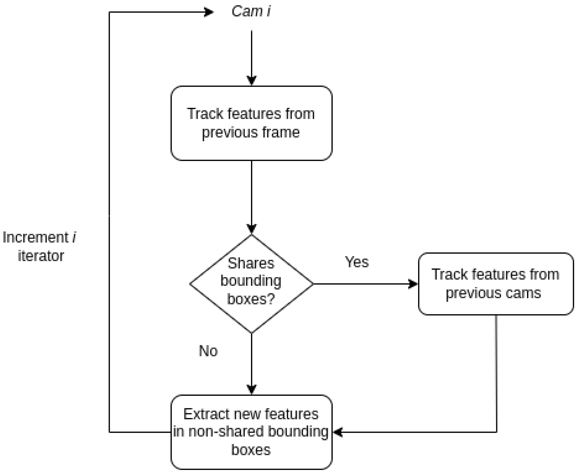
The process works as follows: First, we extract features from the image captured from camera i, excluding the bounding box specified by its parent. Then, we track these features across the bounding boxes of each child camera. If a camera has no parent, we extract features from the entire image. This implementation is illustrated by the flow chart in Figure 1. With this methodology, any multi-camera setup can be accommodated. The relationships between the parent and child cameras, as well as the bounding boxes for the shared fields of view, must be manually provided before running the algorithm. Assuming that the cameras have the same lens, the shared bounding box can be experimentally identified once and remaining consistent over time.

3.2.2. Keyframe Generation

In the original implementation of the algorithm, new landmarks were added, triangulating the unconnected features of the left camera of the stereo setup. When the ratio between the unconnected features of the left camera and the total amount of features tracked in the current frame was below a threshold, the features were triangulated across the previous frame. Then, a new observation was added to the landmark database (see Algorithm 1). Since this approach is only suitable for a stereo camera setup, we propose an implementation to accomplish the landmark database update for a multi-camera setup. For each frame, we evaluate the unconnected points for each camera. For each camera that shares the field of view with another one, we evaluate the ratio between the unconnected and the total amount of features. If at least one of the ratios is below a threshold, we triangulate the unconnected points across the previous frame (see Algorithm 2). In this way, we enable the algorithm to generate keyframes for each camera and not only for the left camera of the original stereo configuration.

Algorithm 1 Original stereo camera keyframe selection.

1: Initialize $connected0\leftarrow 0$ 2: Initialize $unconnected\_obs0\leftarrow 0$ 3: for each feature $kpt\_id$ in left camera observations do 4:    if $lmdb.landmarkExists(kpt\_id)$ then 5:      $tcid\_host\leftarrow lmdb.getLandmark(kpt\_id).host\_kf\_id$ 6:      Add observation to landmark database 7:      Increment $connected0$ 8:    else 9:      Add $kpt\_id$ to $unconnected\_obs0$ 10:    end if 11: end for 12: Compute ratio: $r\leftarrow {\displaystyle \frac{connected0}{connected0+|unconnected\_obs0|}}$ 13: if$r<threshold$and$frames\_after\_kf>min\_frames$then 14:    Triangulate unconnected points across the previous frame 15:    Add new keyframe for left camera 16: end if

Algorithm 2 Multi-camera keyframe selection (ours).

1: Initialize $connected\left[i\right]\leftarrow 0$ for each camera i 2: Initialize $unconnected\_obs\left[i\right]\leftarrow \varnothing$ for each camera i 3: for each camera i do 4:    for each feature $kpt\_id$ in camera i observations do 5:      if $lmdb.landmarkExists(kpt\_id)$ then 6:         $tcid\_host\leftarrow lmdb.getLandmark(kpt\_id).host\_kf\_id$ 7:         Add observation to landmark database 8:         Increment $connected\left[i\right]$ 9:      else 10:         Add $kpt\_id$ to $unconnected\_obs\left[i\right]$ 11:      end if 12:    end for 13: end for 14: for each camera i sharing FOV with another camera do 15:    Compute ratio: $r_i\leftarrow {\displaystyle \frac{connected\left[i\right]}{connected\left[i\right]+|unconnected\_obs[i\left]\right|}}$ 16:    if $r_i<threshold$ then 17:      $take\_kf=true$ 18:    end if 19: end for 20: if$take\_kf$then 21:    for each camera i do 22:      Triangulate unconnected points across the previous frame 23:      Add new keyframe for camera i 24:    end for 25: end if

3.3. Adaptive Threshold for Feature Selection

While a multi-camera setup is very convenient in terms of position accuracy and localization robustness, it is responsible for a high CPU consumption. Especially for applications involving drones, the CPU that can be dedicated to the localization algorithm has to be constrained to enable the onboard computer to handle many other tasks (path planning, obstacle avoidance, data elaboration). The hightest consumption from a VIO algorithm comes from the optical flow generation. One of the most expensive jobs in terms of CPU consumption is related to the tracking of the features. In many situations, a multi-camera setup may overcome the 400% of CPU consumption because all cameras are tracking a hight number of features. To avoid the multi-camera setup tracking too many features, considerably increasing the computational load, we propose a methodology to reduce the number of the tracked features adaptively.

The Basalt algorithm uses a threshold to extract features from an image with FAST algorithm. The threshold defines the minimum difference between the intensity of the candidate pixel and the surrounding pixels and it is initialized to a fixed value. The OpenCV function CV::Fast evaluates this quantity and it can be use to extract only the features that are above a threshold. If the algorithm was not able to find enough features, the threshold is reduced and new features are extracted. In a multi-camera setup, when a high number of features is tracked from one camera to N cameras, the triangulation process will lead to a good estimate of the 3D position of the feature. This will result in a good quality of position accuracy and high localization robustness. In such a situation, tracking features with the other cameras of the setup might be pointless and would increase the CPU loading considerably without any substantial improvements in position accuracy and robustness. We propose an implementation to adaptively select the feature detection threshold for each camera of the configuration. In our implementation, the threshold is divided by the squared root of a scale factor. The scale factor $\tau$ is defined as

$$\tau =e^{-k\left(r-1\right)}$$

(10)

where r is the ratio between the amount of features tracked from the camera i to all its children (cameras that share the field of view with i) and a fixed value that represents the minimum number of features to have $\tau =1$.

$$r={\displaystyle \frac{tracked\_features}{min\_features}}$$

(11)

If $r-1$ is less than 0, we take 0 to always have $r\ge 0$. Therefore, the scale factor $\tau$ is evaluated for the camera i and it will be used to scale the threshold of the camera $i+1$. If the camera i has tracked a number of features close to $min\_features$, the scale factor of the threshold for the camera $i+1$ will be close to 1 and the algorithm will be able to compensate the lack of the feature for the camera i. The $min\_feature$ parameter defines the minimum number of features matched from one camera to another to ensure pose estimate robustness. Since the algorithm tends to accumulate drift when less than 2 or 3 features are matched in a single stereo setup, it has been set to 2 in our code.

In scenarios where one camera detects a large number of features, the other camera will prioritize extracting only high-quality features. As a result, some good-quality features may not be tracked by the second camera. Nevertheless, this implementation is designed to reduce drift accumulation when few features are detected by one camera, while also lowering CPU load in texture-rich environments.

4. Results

4.1. Experimental Setup

The camera used for the experiments is a stereo cameras Oak D-Pro Wide (https://shop.luxonis.com/products/oak-d-pro-w?variant=43715946447071, accessed on 22 May 2025) from Luxonis (Westminister, CO, USA). The tests were conducted by streaming the images at 30 Hz with a 640 × 600 resolution. The ground truth data were obtained using a VICON (Yarnton, Oxfordshire, UK) motion capture system. The recording was performed in a 5 × 6 m room equipped with 10 VICON Bonita 10 cameras mounted on the walls at approximately 2 m above the floor. Vicon Tracker 3.10 was used as the tracking software.

4.2. IMU-Based Feature Prediction

We compare the error in feature position estimates with and without the IMU prediction across three datasets: $Easy$, $Medium$, and $Difficult$. In each dataset, the camera rotates around an axis perpendicular to the image plane, with the rotation speed increasing from the easy to the difficult dataset.

For each dataset, we calculate the Root Mean Square Error (RMSE) between the predicted and actual feature positions. The RMSE is evaluated over 200 frames for each dataset, and the maximum error is also reported. The results are summarized in

Table 2. RMSE comparison: for each dataset, the RMSE and the maximum error of the prediction are reported in pixel units.

Dataset	No IMU		With IMU
	RMSE (pixel)	Max Error (pixel)	RMSE (pixel)	Max Error (pixel)
Easy	0.618	29.931	0.000	6.581
Medium	5.520	81.407	0.003	17.312
Difficult	27.125	195.042	0.134	74.895

.

When using IMU prediction, both the RMSE and the maximum error are significantly reduced. As a result, the IMU prediction helps the algorithm be much less sensitive to fast feature movements, improving its robustness.

To further assess the quality of the prediction, in Figure 2, we present two histograms for each dataset: one for the case with IMU prediction and one without. Since feature tracking can fail due to large position estimation errors, these histograms demonstrate the effectiveness of our IMU-based approach in tracking more features during fast camera movements. Without IMU prediction, the error distribution is highly sensitive to movement speed. In contrast, with IMU prediction, the error remains centered around zero for the majority of features.

4.3. Multi-Camera Implementation

We divide the experimental tests into two typologies: accuracy tests and robustness tests. The accuracy tests provide a comparison of the multi-camera setup with a single stereo camera setup in terms of accuracy. The robustness tests evaluate both setups in scenarios where the stereo camera does not track any features, leading to a rapid accumulation of drift.

4.3.1. Accuracy

We collect the data for two different multi-camera configurations:

• $config1$: two stereo cameras with a tilted angle of 45 degrees with respect to the z axis (Figure 3).
• $config2$: two stereo cameras pointing in opposite directions (Figure 3).

Figure 4 outlines the shared field of view for each camera. The difference between the two configurations is that $config2$ has a wider field compared to $config1$. Instead, in $config1$, we can track features on more than one camera, increasing the observations for the same feature. Figure 3 illustrates the experimental setup. For each configuration, we have collected two different datasets: $Dataset1$ and $Dataset2$ refer to $config1$ while Dataset 3 and Dataset 4 refer to $config2$. Both datasets have been recorded starting from the VICON room and then moving around corridors. After returning to the VICON room we evaluate the accumulated error with respect to the ground truth. This approach was chosen because the corridors where we collected the datasets present challenging conditions for VIO algorithms. For each challenging condition, we provide an approximate estimate in percentage of its presence in the datasets. Note that since all datasets were recorded in similar environments, the reported percentage can be assumed consistent across all datasets.

1.

Featureless walls (white walls): 70%.

2.

Reflecting glazed: 30%.

3.

Areas with poor lighting conditions: 20%.

We specify that some challenging conditions overlap within the datasets. Once returned in the VICON room, we provide a comparison between the ground truth and Basalt trajectory for each dataset. We use the Root Mean Square Error of the Absolute Trajectory Error (RMSE ATE) as the metric to evaluate the accuracy of the estimated trajectory. For each configuration, the ground truth is compared with the following:

1.

The trajectory of the first stereo camera ($Stereo$ 1);

2.

The trajectory of the second stereo camera ($Stereo$ 2);

3.

The trajectory of the multi-camera setup ($Multi-camera$);

4.

The trajectory of the multi-camera setup with the adaptive threshold ($Multi-camera$$AT$) introduced in Section 3.3.

Five trials have been recorded for each case over all datasets to reduce the impact of stochastic data. The results are summarized in Table 3 and Table 4, while in Figure 5, we provide a comparison of the trajectory with the ground truth in the $xy$ plane for two datasets and all setups.

The multi-camera setup has the lowest RMSE ATE for all recorded datasets. The adaptive threshold methodology reduces considerably the computational load and it performs even better than $Multi-camera$ on $Dataset1$. The comparison of the CPU load in Figure 6 shows that both setups are affordable in terms of CPU demand for the most common onboard computers employed for autonomous drones, such as Jetson NVIDIA platforms.

Figure 3. The two configurations of the multi-camera setup: (a) The two stereo cameras have a relative angle of 45 degrees; (b) The two stereo cameras point in different directions.

Figure 3. The two configurations of the multi-camera setup: (a) The two stereo cameras have a relative angle of 45 degrees; (b) The two stereo cameras point in different directions.

Figure 4. Stereo camera configurations: (a) $Stereo$ 1 (cam0 and cam1, yellow field of view) and $Stereo$ 2 (cam2 and cam3, red field of view) with shared field of view between cam1 and cam2 (blue); (b) $Stereo$ 1 and $Stereo$ 2 with non-overlapping fields of view.

Figure 4. Stereo camera configurations: (a) $Stereo$ 1 (cam0 and cam1, yellow field of view) and $Stereo$ 2 (cam2 and cam3, red field of view) with shared field of view between cam1 and cam2 (blue); (b) $Stereo$ 1 and $Stereo$ 2 with non-overlapping fields of view.

Figure 5. Comparison of the trajectory in the $xy$ plane: (a) Trajectories for $config1$ performing on Dataset 2; (b) Trajectories for $config2$ performing on Dataset 3. The trajectories refer to the data collected after returning to the VICON room

Figure 5. Comparison of the trajectory in the $xy$ plane: (a) Trajectories for $config1$ performing on Dataset 2; (b) Trajectories for $config2$ performing on Dataset 3. The trajectories refer to the data collected after returning to the VICON room

Table 3. RMSE ATE comparison (values in meters) for $config2$ with average CPU load percentages. For each dataset, the total traveled distance is indicated in parentheses next to the dataset name.

config1	Dataset 1 (148 m)						Dataset 2 (171 m)						CPU
	1	2	3	4	5	AVG	1	2	3	4	5	AVG
Stereo 1	1.23	1.55	1.41	1.17	1.36	1.34	0.63	0.62	0.56	0.54	0.48	0.57	148%
Stereo 2	1.66	1.92	2.03	1.69	1.75	1.81	1.10	1.40	1.29	1.09	1.33	1.24	151%
Multicam	1.29	1.25	1.19	1.23	1.14	1.22	0.26	0.27	0.35	0.28	0.27	0.29	275%
Multicam AT	0.63	1.00	0.57	0.78	1.01	0.80	0.24	0.53	0.37	0.20	0.36	0.34	205%

1 Results from five trials per configuration. Best average errors highlighted in bold. CPU load measured at 30 Hz with 640 × 600 resolution. 2 All measurements have an uncertainty of 0.05 m.

Table 3. RMSE ATE comparison (values in meters) for $config2$ with average CPU load percentages. For each dataset, the total traveled distance is indicated in parentheses next to the dataset name.

config1	Dataset 1 (148 m)						Dataset 2 (171 m)						CPU
	1	2	3	4	5	AVG	1	2	3	4	5	AVG
Stereo 1	1.23	1.55	1.41	1.17	1.36	1.34	0.63	0.62	0.56	0.54	0.48	0.57	148%
Stereo 2	1.66	1.92	2.03	1.69	1.75	1.81	1.10	1.40	1.29	1.09	1.33	1.24	151%
Multicam	1.29	1.25	1.19	1.23	1.14	1.22	0.26	0.27	0.35	0.28	0.27	0.29	275%
Multicam AT	0.63	1.00	0.57	0.78	1.01	0.80	0.24	0.53	0.37	0.20	0.36	0.34	205%

1 Results from five trials per configuration. Best average errors highlighted in bold. CPU load measured at 30 Hz with 640 × 600 resolution. 2 All measurements have an uncertainty of 0.05 m.

Table 4. RMSE ATE comparison (values in meters) for $config2$ with average CPU load percentages. For each dataset, the total traveled distance is indicated in parentheses next to the dataset name.

config2	Dataset 3 (142 m)						Dataset 4 (164 m)						CPU
	1	2	3	4	5	AVG	1	2	3	4	5	AVG
Stereo 1	0.21	0.29	0.29	0.57	0.33	0.34	0.95	0.92	1.09	0.98	0.96	0.98	109%
Stereo 2	1.13	1.08	0.63	1.16	0.61	0.92	1.12	1.32	1.24	1.25	1.65	1.31	122%
Multicam	0.23	0.22	0.44	0.34	0.27	0.30	0.47	0.63	0.45	0.46	0.47	0.49	210%
Multicam AT	1.30	0.50	0.47	0.89	0.56	0.74	1.85	1.52	1.73	1.55	1.57	1.64	161%

1 Results from five trials per configuration. Best average errors highlighted in bold. CPU load measured at 30 Hz with 640 × 600 resolution. 2 All measurements have an uncertainty of 0.05 m.

Table 4. RMSE ATE comparison (values in meters) for $config2$ with average CPU load percentages. For each dataset, the total traveled distance is indicated in parentheses next to the dataset name.

config2	Dataset 3 (142 m)						Dataset 4 (164 m)						CPU
	1	2	3	4	5	AVG	1	2	3	4	5	AVG
Stereo 1	0.21	0.29	0.29	0.57	0.33	0.34	0.95	0.92	1.09	0.98	0.96	0.98	109%
Stereo 2	1.13	1.08	0.63	1.16	0.61	0.92	1.12	1.32	1.24	1.25	1.65	1.31	122%
Multicam	0.23	0.22	0.44	0.34	0.27	0.30	0.47	0.63	0.45	0.46	0.47	0.49	210%
Multicam AT	1.30	0.50	0.47	0.89	0.56	0.74	1.85	1.52	1.73	1.55	1.57	1.64	161%

1 Results from five trials per configuration. Best average errors highlighted in bold. CPU load measured at 30 Hz with 640 × 600 resolution. 2 All measurements have an uncertainty of 0.05 m.

Figure 6. CPU load comparison: (a) Configuration 1 performance on Dataset 1; (b) Configuration 2 performance on Dataset 3. Both graphs compare the multi-camera setup with and without adaptive threshold, evaluated at 30 Hz streaming with 640 × 600 resolution.

Figure 6. CPU load comparison: (a) Configuration 1 performance on Dataset 1; (b) Configuration 2 performance on Dataset 3. Both graphs compare the multi-camera setup with and without adaptive threshold, evaluated at 30 Hz streaming with 640 × 600 resolution.

4.3.2. Robustness

Since these tests have been conducted to prove the redundancy of our multi-camera implementation, only $config2$ was considered. Indeed, quite similar results would be obtained with $config1$. We recorded a dataset in which Stereo 1 was oriented toward a featureless white wall, while Stereo 2 was directed toward a region with trackable features (see Figure 7). During data collection, the cameras remained stationary. In

Table 5. Comparison of final estimated position (meters) between Stereo 1 and multi-camera setups.

Configuration	3 s			5 s			10 s
	X	Y	Z	X	Y	Z	X	Y	Z
Stereo 1	−1.21	−0.28	4.64	−2.79	−1.02	13.14	−13.99	−33.86	53.94
Multi-camera	−0.04	0.00	0.08	−0.04	−0.08	−0.00	0.00	0.01	0.05

1 All measurements have an uncertainty of 0.05 m.

, we evaluate the positional drift of the estimated trajectory after 3, 5, and 10 s for both Stereo 1 and the multi-camera setups. We report the last estimated position for both configurations. As expected, the estimated position of Stereo 1 rapidly drifts from 0 m due to the lack of tracked features. Thanks to the redundancy introduced by Stereo 2, the estimated position of this setup is stable around 0 m.

Even if these results are obvious once a multi-camera setup is employed, we showed them to highlight the following:

1.

The correctness of the implementation;

2.

The sensitivity of a single stereo camera setup when featureless environments occur, even for few seconds.

5. Discussion

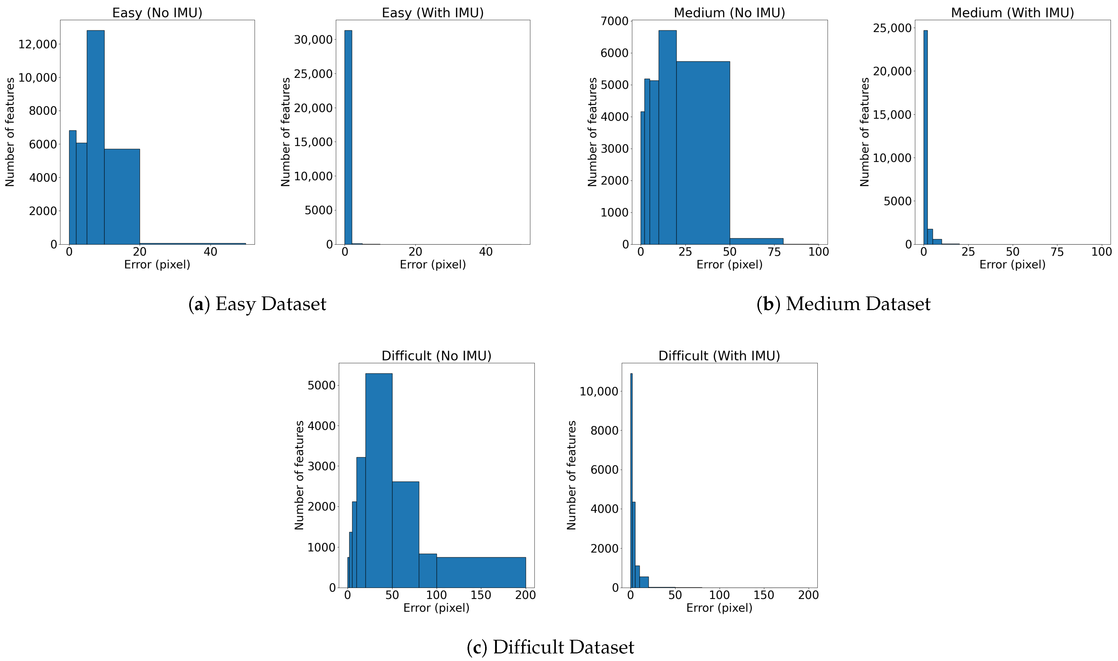
The IMU-based feature prediction significantly enhances feature tracking performance during high-speed maneuvers. Experimental results demonstrate a reduction in the prediction error, leading to more stable tracking of features across consecutive frames. The provided histograms prove the low dispersion of the prediction error when adopting the IMU-based prediction. Considering that the tracking typically fails for errors grater than 30 pixel, in the $Difficult$ dataset, more than 3000 features (out of approximately 15,000 features) would be lost without the IMU-based prediction. This highlights the effectiveness of the implementation during aggressive motions.

The multi-camera implementation presented in this work supports arbitrary configurations. We evaluated its performance in terms of accuracy and robustness across two different configurations. The multi-camera setup offers improved localization accuracy compared to a traditional stereo configuration in challenging environments. However, determining the optimal camera configuration is not straightforward, as it strongly depends on the specific dataset and the characteristics of the surrounding environment.

For all datasets, Stereo 2 shows RMSE ATE greater than Stereo 1. This is because the estimated position of Stereo 2 relies on the IMU of Stereo 1. Since the relative positions of the cameras of Stereo 2 are further from the IMU than the cameras of Stereo 1, larger errors of the relative transformation are introduced during the calibration process. This explains why, in some cases, the RMSE ATE of a single stereo camera is very close to the multi-camera setup.

Since a multi-camera setup relies on the assumption of rigid motion between the cameras, ensuring this rigidity is essential for the algorithm to work properly. The cameras are supposed to be rigidly mounted on the drone, and no relative movement should occur between them during flight. Even without supporting experimental data, a well-built drone should not experience vibrations that significantly affect the relative positions of the cameras or degrade the accuracy of the position estimate.

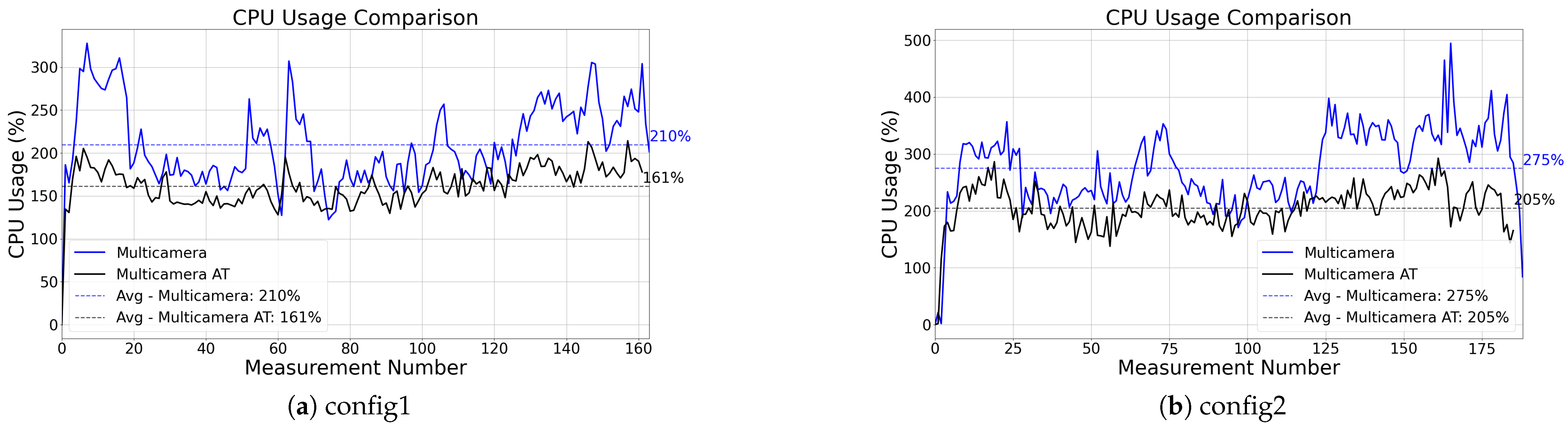
The proposed adaptive threshold methodology contributes to system robustness, reducing the average CPU load by approximately 60%. While the standard multi-camera setup occasionally experiences CPU usage spikes of up to 500%, the integration of adaptive thresholds effectively mitigates these peaks. However, this approach also introduces greater sensitivity to the dataset characteristics, compared to the multi-camera setup.

While the accuracy of the position heavily depends on the quality of the calibration, the multi-camera setup considerably increases the robustness of the localization without being affected by minimal errors in the estimation of the extrinsic calibration parameters. The conducted robustness tests highlight the superior performance of the multi-camera configuration in handling feature-poor environments, while also revealing how quickly the localization accuracy of a stereo setup deteriorates under such challenging conditions.

6. Conclusions

In this paper, we addressed the limitations of VIO-based localization algorithms in scenarios affected by motion blur and low-texture environments. The IMU-based feature prediction improves the robustness of the algorithm when aggressive motions occurs. The multi-camera setup improves the accuracy and the robustness of the position, but minor errors in extrinsic calibration parameters arises when cameras are far apart from each other, penalizing the accuracy of the estimated position. Since the algorithm was designed to be executed on board of a drone, special attention was paid to minimizing CPU usage. The proposed improvements result in enhanced accuracy and robustness while maintaining a processing load compatible with typical onboard computers used in autonomous drones, such as the NVIDIA Jetson platforms.