A Partitioned Operational Space Approach for Singularity Handling in Six-Axis Manipulators

Abstract

Task prioritization for inverse kinematics can be a powerful tool for realizing objectives in robot manipulation. This is particularly true for robots with redundant degrees of freedom, but it can also help address a debilitating singularity in six-axis robots. A roll-pitch-roll wrist is especially problematic for any six-axis robot because it produces a “gimbal-lock” singularity in the middle of the wrist workspace when the roll axes align. A task priority methodology can be used to realize only the achievable components of the commanded motion in the reduced operational space of a manipulator near singularities while phasing out the uncontrollable direction. In addition, this approach allows the operator to prioritize translation and rotation in the region of singularities. This methodology overcomes a significant drawback to the damped least-squares method, which can produce tool motion that deviates significantly from the desired path even in directions that are controllable. The approach used here reduces the operational space near the wrist singularity while maintaining full command authority over tool translation. The methodology is demonstrated in simulations conducted on a six degree-of-freedom Motoman MH250 manipulator.

1. Introduction

Robot manipulators are typically controlled by specifying the desired Cartesian velocities of the end-effector, which are then mapped into joint rate commands. This process, referred to as “resolved-rate control”, runs into difficulty when the “Jacobian” mapping between joint and Cartesian space becomes singular. A singularity occurs when joint motions become linearly dependent, which causes the rank of the Jacobian to collapse. Singularities can occur either at the workspace boundary, such as when the arm is fully extended, or internal to the workspace, such as when two joint axes align. If the singularities are not addressed in the inverse kinematics, then large joint velocities and errors in the end-effector trajectory can result.

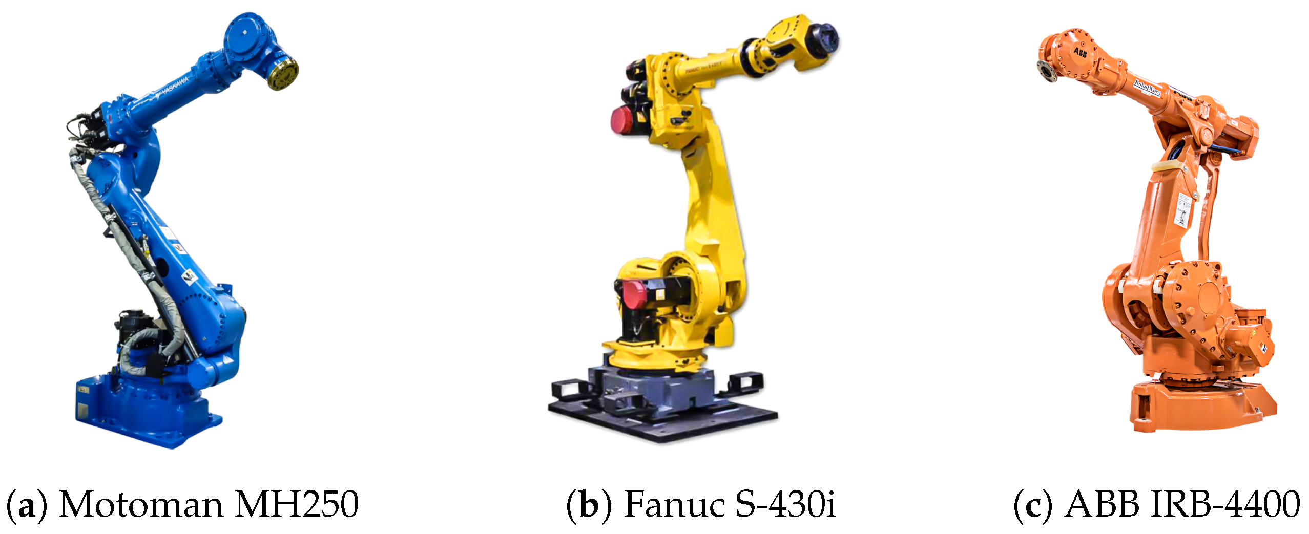
When a six-axis manipulator encounters a singularity, it can be particularly catastrophic since it results in the loss of a tool Cartesian translational or rotational Degree(s) of Freedom (DOF). For industrial manipulators such as those shown in Figure 1 with a yaw-pitch-pitch arm and roll-pitch-roll (RPR) wrist, the singularities occur when [1]: (a) the elbow pitch causes the shoulder, elbow, and wrist pitch joints to be co-linear, (b) the wrist (intersection of joints 4-5-6) falls on the joint 1 axis, and (c) the wrist pitch causes joints 4 and 6 to align. The elbow pitch singularity causes nearly full arm extension and therefore is most practically avoided by not commanding the robot outside its reachable workspace. The wrist on joint 1 axis singularity is commonly avoided by keeping the task forward so that the tool does not need to reach above the robot. However, the wrist singularity is extremely difficult to avoid because it occurs in the center of the wrist rotation workspace and can occur anywhere in the reachable workspace of the tool.

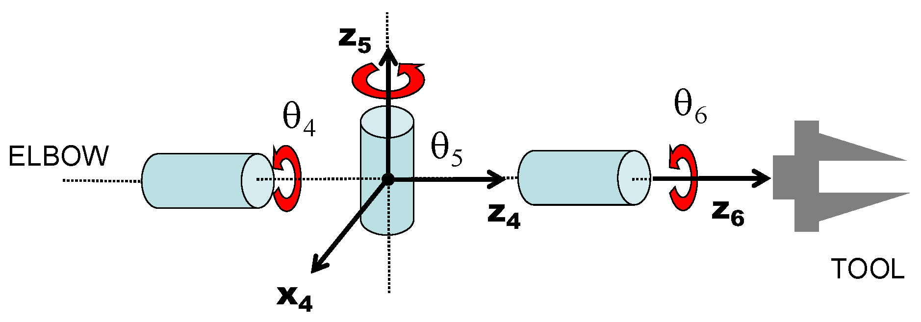
The RPR wrist becomes singular when the wrist pitch angle is $0^{\circ }$ so that the forearm (${\widehat{z}}_4$) and hand roll (${\widehat{z}}_6$) axes align (see Figure 2). This neutralizes rotation about an axis (${\widehat{x}}_4$) that is perpendicular to the plane containing the two roll and pitch (${\widehat{z}}_5$) axes. This singularity is particularly troublesome since it is in the middle of the wrist workspace and wrist abduction/adduction is common throughout the course of a task. Since the singularity cannot be avoided for a six-degree-of-freedom (DOF) robot, then the ill-conditioning of the Jacobian must be handled if the manipulator is to remain in resolved-rate mode.

By far the most common approach in use is the damped least-squares (DLS) method, which modifies the minimum singular value of the Jacobian so that it is nonsingular throughout the workspace ([2,3,4]). The challenge is in selecting a suitable damping factor that gives good behavior in the neighborhood of all singularities without sacrificing too much accuracy. To help resolve this, a weighting matrix can be applied to the Jacobian to deemphasize movement in certain directions [5] or to use the inertia to reduce acceleration near singularities [1]. However, the distortion of the Jacobian mapping can produce motion even in directions that are controllable. This “uncommanded” motion can result in inadvertent collisions of the tool with the worksite during close proximity tasks.

Another approach to handling singularities is to eliminate the degenerate component of the motion near the singularity thereby preventing the buildup of large velocities [6,7]. The row of the Jacobian corresponding to the singular direction is eliminated, and then the pseudoinverse of the degenerate Jacobian is used to find the mapping between the Cartesian and joint velocities. This procedure has the advantage of eliminating the singular behavior while maintaining a least-squares fit to the desired Cartesian path. However, this requires a priori knowledge of the singularity locations, and several investigators have reported “jerkiness” on the singularity boundary while transitioning between the full and degenerate Jacobians to compute the inverse kinematics.

Other investigators have sought to resolve the spherical wrist singularity in six-axis manipulators by adding a virtual (nonphysical) axis at the end-effector [8]. Referred to as the Virtual Redundant Axis Method (VRAM), the virtual joint absorbs the Cartesian tracking errors created in the singular direction of the wrist when the joint axes align. Since the robot now has kinematic redundancy by virtue of the additional joint, a weighted DLS solution is then implemented in which the physical uncontrollable direction is heavily penalized. This method has also been recently generalized to other singularities in serial robots [9]. However, the VRAM requires additional computation, and like the DLS method, can still produce tracking errors in the controllable direction.

The objective of this research is to address the abovementioned deficiencies in singularity avoidance algorithms currently being used for this class of nonredundant robots. While the Task Priority Inverse Kinematics (TPIK) method has been previously used for kinematically redundant robots [10,11], applying it to singularity handling for a 6-DOF robot has not been previously done. The new approach is able to preserve the Cartesian path in controllable directions (in a specified order of priority) while circumventing singularities without a priori knowledge of their locations.

The article begins with a brief review of resolved-rate control and the task priority method in Section 2. The specific algorithm and equations for controlling a six-axis robot are presented in Section 3. Simulations for the Motoman MH250 manipulator [Yaskawa Electric Corp., Kitakyushu, Fukuoka, Japan] are given in Section 4. Results and conclusions are presented in Section 5. The kinematics and singularity analysis for the Motoman MH250 manipulator are presented in Appendix A and Appendix B, respectively. The Jacobian and manipulability calculations needed by the task priority and projection method are given in Appendix C. Functions implemented by the algorithms are given in Appendix D.

2. Task Priority Inverse Kinematics and Task Projection Theory

The joint position solver is situated between the Cartesian Rate Limiter (CRL) and the Joint Velocity Norm Limiter (JVNL), as illustrated in Figure 3. The reference Cartesian position input on the left is derived by integrating the commanded Cartesian position changes, $\Delta x_{ref}^T\equiv [\delta p_{ref}^T\delta r_{ref}^T]$, where the components represent the position and angle-axis “twist”, respectively. The $k^{th}$ step of the integration is as follows:

$$\begin{array}{c}\hfill x_{re{f}_{k+1}}=x_{re{f}_k}+\Delta x_{re{f}_k}\end{array}$$

(1)

where $x_{re{f}_k}$ is the last reference joint position.

The summer block calculates the difference between the reference task space pose, ⁰$x_{ref}$, and the task space pose, ⁰$x_{fk}$, calculated from the forward kinematics of the last joint command issued by the norm-limited output of the solver, $q_{ik}$. The CRL then enforces a saturation limit to prevent excessive Cartesian rate inputs to the position solver. The JVNL applies a saturation limit to the difference between the output of the joint position solver, $q_{cmd}$, and the previous output of the joint velocity norm limiter, $q_{ik}$, to maintain the norm of the joint position change within specified limits. Thus, the input to the position solver, ⁰$x_{cmd}$, takes into account not just the trajectory ⁰$x_{ref}$ but also any Cartesian position errors that accrue due to Cartesian or joint rate limiting external to the solver and singularity avoidance internal to the solver.

A Newton–Raphson iteration technique is then used within the position solver to converge on the joint solution based on the inverse Jacobian as follows:

$$\begin{array}{c}\hfill q_{{cmd}_{k+1}}=q_{{cmd}_k}+J{\left(q_{{cmd}_k}\right)}^{-1}(x_{cmd}-f\left(q_{{cmd}_k}\right))\end{array}$$

(2)

where $x_{cmd}$ is the commanded tool pose from the CRL, $q_{{cmd}_k}$ is the estimate of the commanded joint position in the kth step of the iteration, and $f(·)$ represents the forward kinematics.

The classical approach is for the velocity solver to invert the Jacobian using a singularity-robust inverse method such as damped least-squares [2,3]. Another option is to break up the inverse kinematics into tasks, which are assigned a priority for singularity avoidance [12,13,14]. Thus, a singularity in the higher order task is prevented by altering the desired path of a lower priority task. This secondary task correction uses a task projection on the manipulability boundary to prevent the manipulability index from penetrating the boundary. In effect, the manipulability constraint is dynamically reallocated to become the highest priority task when it is active [13].

2.1. Task Priority Inverse Kinematics

In the TPIK approach [15], the task space, x, is divided into subspaces, $x_i$, where i denotes the order of importance. The joint velocities $\dot{q}\in {\mathbb{R}}^n$ are related to the task space velocities ${\dot{x}}_i\in {\mathbb{R}}^{m_i}$ by

$$\delta x_i=J_i\left(q\right)\delta q$$

(3)

where $J_i\left(q\right)\in {\mathbb{R}}^{m_i\times n}$ is the Jacobian of the task subspace variable, $x_i$. Using this task decomposition eventually leads to the following recursive formulation for the inverse kinematics [13,16,17]

$$\left\{\begin{array}{c}{\widehat{J}}_i=J_i{N}_{i-1}\hfill \\ N_i=N_{i-1}-{{\widehat{J}}_i}^{†}{\widehat{J}}_i\hfill \\ \delta {\widehat{x}}_i=\delta x_i-J_i\delta q_{i-1}\hfill \\ \delta q_i=\delta q_{i-1}+{{\widehat{J}}_i}^{†}\delta {\widehat{x}}_i\hfill \end{array}\right.,\left\{\begin{array}{c}\delta q_0=0\hfill \\ N_0=I_n\hfill \end{array}\right..$$

(4)

where $J_i^{†}\left(q\right)\in {\mathbb{R}}^{n\times m_i}$ is the right pseudoinverse of $J_i\left(q\right)$.

The prioritized task inverse kinematics process for three tasks is shown in Figure 4. The change in joint positions for first task, $\delta q_1$, is obtained by multiplying the pseudoinverse of $J_1$ by the desired change for Task 1. The effect of $\delta q_1$ on Task 2 is found by multiplying $J_2$ by $\delta q_1$, which is then subtracted from the desired change for Task 2 to give the modified change for the second task, $\delta {\widehat{x}}_2=\delta x_2-J_2\delta q_1$. This is then multiplied by the pseudoinverse of ${\widehat{J}}_2^{†}$ to give the joint change for Task 2, $\delta q_2$. Similarly, the effect of the total joint change on Task 3 is subtracted from the desired change for Task 3 to give the joint change for Task 3, $\delta q_3={\widehat{J}}_3^{†}[\delta x_3-J_3(\delta q_1+\delta q_2)]$. Note that ${\widehat{J}}_i$ strips out the range space of the Jacobians from the previous tasks to ensure that any solution for $\delta q_i$ cannot affect the previous tasks.

2.2. Singularity Avoidance by Task Projection

The task inverse kinematics process fails when a task Jacobian in Equation (4) is not invertible. Near a singularity, the task reconstruction method is used to alter the path to go around the singularity [13,14]. The manipulability index, $m\left(q\right)$, is defined as follows

$$m\left(q\right)=\sqrt{det\left[J{J}^T\right]}$$

(5)

which is a continuous, nonnegative scalar that equals zero only when the Jacobian is not full rank [18]. Since m is the product of the singular values of J, it is also a measure of the distance from the singularity [13]. If the singular value in any direction is 0, then the manipulability will also be 0.

A small variation in the manipulability index is computed from:

$$\delta m\left(q\right)={\displaystyle \frac{\partial m\left(q\right)}{\partial q}}\delta q={\displaystyle \frac{\partial m\left(q\right)}{\partial q}}{J}^{†}\delta x$$

(6)

For $\delta m\left(q\right)$ to be equal to 0, this implies that the task displacement must be orthogonal to the vector, $n_m\equiv {\displaystyle \frac{\partial m\left(q\right)}{\partial q}}{J}^{†}$. In other words, $\delta x$ must be tangent to the surface defined by:

$$\left({\displaystyle \frac{\partial m\left(q\right)}{\partial q}}{J}^{†}\right)·\delta x=0$$

(7)

where $x\in {\mathbb{R}}^m$. Observing now that $n_m$ must be normal to the surface, then the projection of the task on the singularity surface is as follows:

$$\delta x_p=\delta x-(\delta x·n_m)n_m=(I_m-n_m{n}_m^T)\delta x$$

(8)

Thus, $\delta x_p$ is the component of the task change that avoids the singularity. Figure 5 is an illustration of the reconstructed path as it intersects and then moves along the manipulability boundary $m=\overline{m}$ to avoid the singularity.

2.3. Task Priority with Task Projection

The task priority decomposition with the task projection incorporated for singularity avoidance is displayed in the block diagram shown in Figure 6. This particular formulation implements singularity avoidance for Tasks 1 and 2 and no singularity avoidance for Task 3. The velocity decomposition for each task can be broken down into a three-step process represented by the different blocks: task correction (previous task adjustment), task reconstruction (singularity avoidance), and Jacobian pseudoinverse (joint adjustment). Variable data enter from the left and calculated values exit from the right. Dashed line inputs indicate position-dependent Jacobian and manipulability input data that can be calculated by a processor at a slower rate.

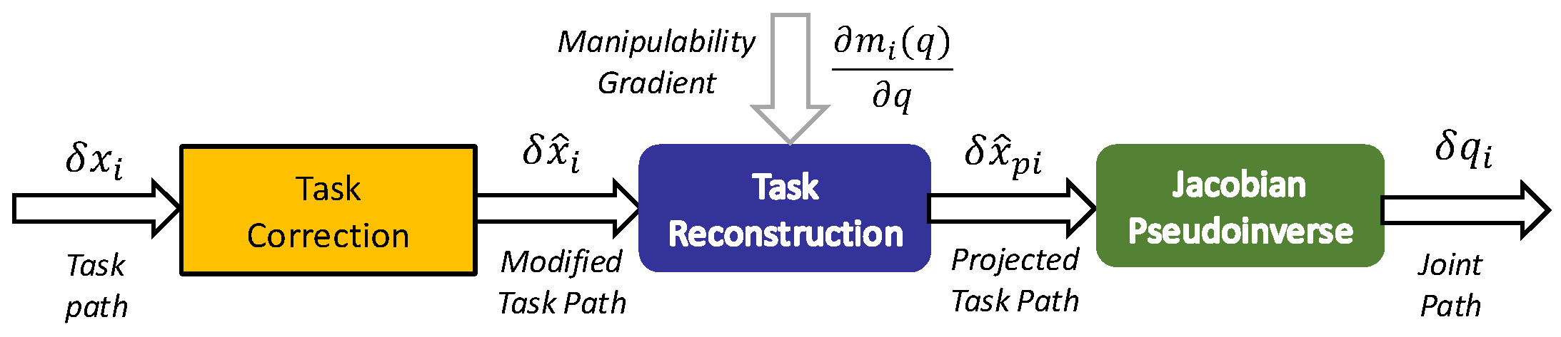
For example, the process is illustrated for Task i = 2 is illustrated with the aid of Figure 7. The first step is to remove effect of previous task(s) from the current task using the following

$$\delta {\widehat{x}}_2=\delta x_2-J_2[J_1^{†}\delta x_1]$$

(9)

The quantity in brackets is the change in joint positions $\delta q_1$ due to achieving Task 1. Therefore, multiplication by $J_2$ yields the change in Task 2 due to application of Task 1.

The second step is to alter the path to circumvent a singularity:

$$\delta {\widehat{x}}_{p2}=\delta {\widehat{x}}_2-k_1[(\delta {\widehat{x}}_2·n_m)n_m]$$

(10)

The quantity in brackets is the component of Task 2 that is in the direction of the gradient of the singularity, $n_m$. If the dot product is negative, then the component is toward the singularity, and a portion of this is removed depending on how close it is to the singularity boundary. This behavior is achieved through the dynamic correction gain $k_1$ (see Appendix D.1).

The third step is to apply the Task 2 Jacobian pseudoinverse to the Task 2 command to obtain the change in joint positions to achieve Task 2:

$$\delta q_2={\widehat{J}}_2^{†}\delta {\widehat{x}}_{p2}$$

(11)

where ${\widehat{J}}_2^{†}$ is the Jacobian for Task 2 with the portion of it that would alter Task 1 removed.

2.4. Manipulability Gradients for Task Reconstruction

Denote the manipulability operator $\mu (·)$ for a Jacobian J as

$$\mu \left(J\right)\equiv \sqrt{det\left(J{J}^T\right)}$$

(12)

The derivative of measure of manipulability can be expressed with respect to the already-known quantities, $\mu \left(J\right)$ and $J^{†}$, plus the derivative of each element of J with respect to $q_k$, which can be easily computed symbolically [14,19]:

$${\displaystyle \frac{\partial \mu \left(J\right)}{\partial q_k}}=\mu \left(J\right)·\mathrm{trace}\left\{{\displaystyle \frac{\partial J}{\partial q_k}}{J}^{†}\right\}$$

(13)

where the right pseudoinverse of J is given by

$$J^{†}\equiv J^T{\left(J{J}^T\right)}^{-1}$$

(14)

The computations can also be performed in any coordinate frame, which can significantly reduce mathematical operations as detailed in Appendix C.

In the case of multiple tasks, the measure of manipulability for a given task, $m_i$, is given by

$$m_i\left(q\right)\equiv \mu \left({\widehat{J}}_i\right)=\sqrt{det\left({\widehat{J}}_i{\widehat{J}}_i^T\right)}$$

(15)

In the above formulation, the computation of $\partial m_i\left(q\right)/\partial q$ is not immediately obvious. Defining the augmented Jacobian $S_i$ for Task i as

$$S_i=\left[\begin{array}{c}{J}_1\\ ...\\ J_{i-1}\\ J_i\end{array}\right]$$

(16)

where $S_1=J_1$. The relationship between the task manipulability and the augmented task manipulability can be determined as follows [14]:

$$m_j={\displaystyle \frac{\mu \left(S_j\right)}{\mu \left(S_{j-1}\right)}}forj>1$$

(17)

where $m_1=\mu \left(S_1\right)$. Taking the partial of Equation (17) with respect to the configuration vector q:

$${\displaystyle \frac{\partial \mu \left({\widehat{J}}_j\right)}{\partial q}}={\displaystyle \frac{1}{\mu \left(S_{j-1}\right)}}\left({\displaystyle \frac{\partial \mu \left(S_j\right)}{\partial q}}-{\displaystyle \frac{\partial \mu \left(S_{j-1}\right)}{\partial q}}\mu \left({\widehat{J}}_j\right)\right)$$

(18)

The partials of the manipulability for the augmented Jacobian $\partial \mu \left(S_j\right)/\partial q$ can be easily computed in closed symbolic form or numerically using again Equation (13):

$${\displaystyle \frac{\partial \mu \left(S_j\right)}{\partial q_k}}=\mu \left(S_j\right)·\mathrm{trace}\left\{{\displaystyle \frac{\partial S_j}{\partial q_k}}{S}_j^{†}\right\}$$

(19)

Since $m_i\left(q\right)\equiv \mu \left({\widehat{J}}_i\right)$ via Equation (15), Equation (18) can be applied recursively to each task as outlined in Algorithm A3.

3. Program and Procedure

The basic procedure for TPIK with three tasks is illustrated in Figure 8. The Jacobian pseudoinverse for each task is used to derive the least-squares solution of the joint angles to accomplish the task. The task decomposition into joint space is performed in numerical order so that all of the joint DOF are used to achieve the first task then the second task and finally the third task. If there are no singularities along the trajectory, then the order becomes irrelevant and the full task trajectory is achieved. If a singularity is encountered, then the task is projected on the singularity surface using the manipulability gradient. Since the Jacobians and manipulabilities are only position-dependent, they may be computed at a slower rate. After the change in joint angles is computed, the norm of the task error is compared with the threshold. If the error is within the threshold, then the final solution is achieved. If not, then another iteration is performed as long as the maximum number of iterations is not exceeded.

3.1. Position-Dependent Data Input (Slow Rate Loop)

The position-dependent data structure contains both Jacobian and manipulability calculations that only depend on the joint position q and can therefore be computed at a slower rate than velocity dependent terms.

3.1.1. Task Jacobians

The tasks are chosen from highest to lowest priority as follows: (1) the three components of tool position, (2) the y and z-components of the tool rotation, and (3) the x-component of tool rotation all in forearm frame 4. The task Jacobians are, hence, computed and assigned the following task priority:

$$\begin{array}{ccc}\hfill J_1& =& {\phantom{.}}^4{J}_t\left(\theta \right)\hfill \end{array}$$

(20)

$$\begin{array}{ccc}\hfill J_2& =& {\phantom{.}}^4{J}_r{\left(\theta \right)}_{row2,3}\hfill \end{array}$$

(21)

$$\begin{array}{ccc}\hfill J_3& =& {\phantom{.}}^4{J}_r{\left(\theta \right)}_{row1}\hfill \end{array}$$

(22)

The translation and rotation Jacobians, ⁴$J_t\left(\theta \right)\in {\Re }^{3\times 6}$ and ⁴$J_r\left(\theta \right)\in {\Re }^{3\times 6}$, are computed in frame 4 using the cross product method as outlined in Appendix A.2.

The modified Jacobian, ${\widehat{J}}_i$, and manipulability, $m_i$, for each task i are derived from the task Jacobians, $J_i$, using Equations (4) and (15):

Task 1:

$$\begin{array}{ccc}\hfill {\widehat{J}}_1& =& J_1{N}_0\hfill \end{array}$$

(23)

$$\begin{array}{ccc}\hfill m_1& =& \sqrt{det\left({\widehat{J}}_1{\widehat{J}}_1^T\right)}\hfill \end{array}$$

(24)

$$\begin{array}{ccc}\hfill N_1& =& N_0-{\widehat{J}}_1^{†}{\widehat{J}}_1\hfill \end{array}$$

(25)

Task 2:

$$\begin{array}{ccc}\hfill {\widehat{J}}_2& =& J_2{N}_1\hfill \end{array}$$

(26)

$$\begin{array}{ccc}\hfill m_2& =& \sqrt{det\left({\widehat{J}}_2{\widehat{J}}_2^T\right)}\hfill \end{array}$$

(27)

$$\begin{array}{ccc}\hfill N_2& =& N_1-{\widehat{J}}_2^{†}{\widehat{J}}_2\hfill \end{array}$$

(28)

Task 3:

$$\begin{array}{ccc}\hfill {\widehat{J}}_3& =& J_3{N}_2\hfill \end{array}$$

(29)

$$\begin{array}{ccc}\hfill m_3& =& \sqrt{{\widehat{J}}_3{\widehat{J}}_3^T}\hfill \end{array}$$

(30)

Note that since ${\widehat{J}}_3$ is a row vector, the product in Equation (30) is a scalar and therefore taking the determinant is unnecessary.

3.1.2. Manipulability Gradients

The augmented Jacobians $S_i$ are constructed as:

$$S_1=J_1,S_2=\left[\begin{array}{c}{J}_1\\ J_2\end{array}\right],S_3=\left[\begin{array}{c}{J}_1\\ J_2\\ J_3\end{array}\right]$$

(31)

Calculate the right pseudoinverses of the augmented Jacobians $S_i^{†}$:

$$S_i^{†}=S_i^T{\left(S_i{S}_i^T\right)}^{-1}$$

(32)

and the augmented Jacobian manipulabilities $\mu \left(S_i\right)$:

$$\mu \left(S_i\right)=\sqrt{det\left(S_i{S_i}^T\right)}$$

(33)

Note that since $S_i{S}_i^T$ is symmetric, the Cholesky Decomposition can be used to compute the inverse [20]. It is much more efficient than singular value decomposition [21], and it has the added benefit of returning its determinant which can be used to compute the manipulability. The task manipulabilities are computed as follows:

$$m_1=\mu \left(S_1\right),m_2={\displaystyle \frac{\mu \left(S_2\right)}{\mu \left(S_1\right)}},m_3={\displaystyle \frac{\mu \left(S_3\right)}{\mu \left(S_2\right)}}$$

(34)

Note that although the manipulabilities have already been defined by Equations (24), (27), and (30), Equation (34) is a secondary method of calculation that can serve as an error check.

The gradient of the augmented Jacobian $S_i$ with respect to each joint angle ${\theta }_k$ results in a matrix the same dimension as $S_i$:

$$\begin{array}{ccc}\hfill {\displaystyle \frac{\partial S_1}{\partial {\theta }_k}}& =& {\displaystyle \frac{{\partial }^3{J}_1}{\partial {\theta }_k}}k=1\dots N\hfill \\ \hfill {\displaystyle \frac{\partial S_2}{\partial {\theta }_k}}& =& \left[\begin{array}{c}{\displaystyle \frac{{\partial }^3{J}_1}{\partial {\theta }_k}}\\ {\displaystyle \frac{{\partial }^3{J}_2}{\partial {\theta }_k}}\end{array}\right]k=1\dots N\hfill \\ \hfill {\displaystyle \frac{\partial S_3}{\partial {\theta }_k}}& =& \left[\begin{array}{c}{\displaystyle \frac{{\partial }^3{J}_1}{\partial {\theta }_k}}\\ {\displaystyle \frac{{\partial }^3{J}_2}{\partial {\theta }_k}}\\ {\displaystyle \frac{{\partial }^3{J}_3}{\partial {\theta }_k}}\end{array}\right]k=1\dots N\hfill \end{array}$$

(35)

where ${\displaystyle \frac{{\partial }^3{J}_t}{\partial {\theta }_k}}$ and ${\displaystyle \frac{{\partial }^3{J}_r}{\partial {\theta }_k}}$ needed to compute the gradients in Equation (35) are given in Appendix C.

The gradients of the augmented Jacobian manipulability $S_i$ with respect to joint angle ${\theta }_k$ are calculated as follows:

$${\displaystyle \frac{\partial \mu \left(S_i\right)}{\partial {\theta }_k}}=\mu \left(S_i\right)·\mathrm{trace}\left\{{\displaystyle \frac{\partial S_i}{\partial {\theta }_k}}{S}_i^{†}\right\}$$

(36)

These calculations are carried out numerically using the algorithm for the function $DSDQ\left(\right)$ as outlined in Appendix D.3. The augmented Jacobian manipulability gradient is then formulated by assembling the elements into a vector for N joints as follows:

$${\displaystyle \frac{\partial \mu \left(S_i\right)}{\partial q}}=\left[\begin{array}{c}{\displaystyle \frac{\partial \mu \left(S_i\right)}{\partial {\theta }_1}}\\ ⋮\\ {\displaystyle \frac{\partial \mu \left(S_i\right)}{\partial {\theta }_N}}\end{array}\right]$$

(37)

Finally, the task manipulability gradients are given by:

$$\begin{array}{ccc}\hfill {\displaystyle \frac{\partial m_1}{\partial q}}& =& {\displaystyle \frac{\partial \mu \left(S_1\right)}{\partial q}}\hfill \end{array}$$

(38)

$$\begin{array}{ccc}\hfill {\displaystyle \frac{\partial m_2}{\partial q}}& =& {\displaystyle \frac{1}{\mu \left(S_1\right)}}\left({\displaystyle \frac{\partial \mu \left(S_2\right)}{\partial q}}-{\displaystyle \frac{\partial \mu \left(S_1\right)}{\partial q}}{m}_2\right)\hfill \end{array}$$

(39)

$$\begin{array}{ccc}\hfill {\displaystyle \frac{\partial m_3}{\partial q}}& =& {\displaystyle \frac{1}{\mu \left(S_2\right)}}\left({\displaystyle \frac{\partial \mu \left(S_3\right)}{\partial q}}-{\displaystyle \frac{\partial \mu \left(S_2\right)}{\partial q}}{m}_3\right)\hfill \end{array}$$

(40)

3.2. Velocity Solver (Fast Rate Loop)

The tasks are chosen from highest to lowest priority as follows: (1) the three components of tool position, (2) the y and z-components of the tool rotation, and (3) the x-component of tool rotation all in forearm frame 4. Thus, the algorithm will maintain tool position before it relinquishes control to tool orientation. Then, the tool rotation is broken down into the y–z plane that is controllable and the x-direction that is uncontrollable at the wrist pitch singularity with the higher priority given to the former.

3.2.1. Initialization

The input to the velocity solver is a twist in the base frame, ${\delta }^{0}x$, which is the combined vector of linear and angular velocities multiplied by the sample period as follows:

$${\delta }^{0}x=\left[\begin{array}{c}{\delta }^0{p}_{tool}\\ {\delta }^0{r}_{tool}\end{array}\right]$$

(41)

where ${\delta }^0{p}_{tool}$ represents a free vector in Cartesian space and ${\delta }^0{r}_{tool}$ is an infinitesimal angle multiplied by a unit axis of rotation. Multiply the components of the twist by the rotation matrix from frame 0 to frame 4 to get the twist in frame 4:

$$\begin{array}{ccc}\hfill {\delta }^4{p}_{tool}& =& {\phantom{.}}^4{R}_0{\delta }^0{p}_{tool}\hfill \\ \hfill {\delta }^4{r}_{tool}& =& {\phantom{.}}^4{R}_0{\delta }^0{r}_{tool}\hfill \end{array}$$

(42)

Next, set the change in the each task position as follows:

$$\delta x_1=\left[\begin{array}{c}{\delta }^4{p}_{too{l}_x}\\ {\delta }^4{p}_{too{l}_y}\\ {\delta }^4{p}_{too{l}_z}\end{array}\right]\delta x_2=\left[\begin{array}{c}{\delta }^4{r}_{too{l}_y}\\ {\delta }^4{r}_{too{l}_z}\end{array}\right]\delta x_3={\delta }^4{r}_{too{l}_x}$$

(43)

3.2.2. Execute Task Decomposition

Initialize the joint position change to zero, $\delta q_0=0$:

Task 1:

$$\begin{array}{ccc}\hfill \delta {\widehat{x}}_1& =& \delta x_1-J_1\delta q_0\hfill \end{array}$$

(44)

$$\begin{array}{ccc}\hfill \delta {\widehat{x}}_{1p}& =& TR\left(m_1,{{\widehat{J}}_1}^{†T}{\displaystyle \frac{\partial m_1}{\partial q}},\delta {\widehat{x}}_1,{\overline{m}}_1,m_{\sigma 1},{\overline{n}}_m,{\overline{m}}_{\Delta }\right)\hfill \end{array}$$

(45)

$$\begin{array}{ccc}\hfill \delta q_1& =& \delta q_0+{\widehat{J}}_1^{†}\delta {\widehat{x}}_{1p}\hfill \end{array}$$

(46)

Task 2:

$$\begin{array}{ccc}\hfill \delta {\widehat{x}}_2& =& \delta x_2-J_2\delta q_1\hfill \end{array}$$

(47)

$$\begin{array}{ccc}\hfill \delta {\widehat{x}}_{2p}& =& TR\left(m_2,{{\widehat{J}}_2}^{†T}{\displaystyle \frac{\partial m_2}{\partial q}},\delta {\widehat{x}}_2,{\overline{m}}_2,m_{\sigma 2},{\overline{n}}_m,{\overline{m}}_{\Delta }\right)\hfill \end{array}$$

(48)

$$\begin{array}{ccc}\hfill \delta q_2& =& \delta q_1+{\widehat{J}}_2^{†}\delta {\widehat{x}}_{2p}\hfill \end{array}$$

(49)

Task 3:

$$\begin{array}{ccc}\hfill \delta {\widehat{x}}_3& =& \delta x_3-J_3\delta q_2\hfill \end{array}$$

(50)

$$\begin{array}{ccc}\hfill \delta {\widehat{x}}_{3p}& =& S_{04}(m_3,0,1,{\overline{m}}_3,{\overline{m}}_3+m_{\sigma 3})\delta {\widehat{x}}_3\hfill \end{array}$$

(51)

$$\begin{array}{ccc}\hfill \delta q_3& =& \delta q_2+{\widehat{J}}_3^{†}\delta {\widehat{x}}_{3p}\hfill \end{array}$$

(52)

with $S_{04}$ defined in Equation (A23). The change in joint position output from Task 3, $\delta q_3$, is the cumulative change in joint position for a single iteration of the position solver. Note that no singularity avoidance is used for Task 3. Instead, $\delta {\widehat{x}}_{3p}$ is phased out starting at the transition boundary and completely dropped at the manipulability boundary.

3.3. Joint Velocity Norm Limiter

The purpose of the JVNL is to limit the change in joint positions output by the position solver. While the velocity solver will result in continuous velocities, it can produce large changes in joint velocity during singularity avoidance. The norm limiter limits the magnitude of the joint position changes to help smooth that behavior.

The allowable change in the joint position norm per control cycle is calculated based the selected joint velocity norm limit ${\dot{\theta }}_{NormLim}$ and the control cycle period $\Delta t$:

$${\Vert \delta \theta \Vert }_{limit}={\dot{\theta }}_{NormLim}\ast \Delta t$$

(53)

Let the change in the position solver output from the previous cycle be $\delta {\theta }_{cmd}$:

$$\delta {\theta }_{cmd}={\theta }_{cmd}-{\theta }_{cm{d}_{prev}}$$

(54)

This change is then clamped to the limit if it exceeds the above threshold as follows:

$$\delta {\theta }_{jvnl}=\left\{\begin{array}{cc}{\displaystyle \frac{{\Vert \delta \theta \Vert }_{limit}}{\Vert \delta {\theta }_{cmd}\Vert }}\delta {\theta }_{cmd}\hfill & \Vert \delta {\theta }_{cmd}\Vert >{\Vert \delta \theta \Vert }_{limit}\hfill \\ \delta {\theta }_{cmd}\hfill & \Vert \delta {\theta }_{cmd}\Vert \le {\Vert \delta \theta \Vert }_{limit}\hfill \end{array}\right.$$

(55)

where $\Vert {\theta }_{cmd}\Vert =\sqrt{{\displaystyle \sum _{i=1}^n}{\theta }_{cm{d}_i}^2}$. Then, the clamped final output ${\theta }_{ik}$ is given by:

$${\theta }_{ik}={\theta }_{{cmd}_{last}}+\delta {\theta }_{jvnl}$$

(56)

The previous joint position solver output is saved as ${\theta }_{{cmd}_{prev}}={\theta }_{cmd}$, and the JVNL outputs the norm limited joint position ${\theta }_{ik}$.

4. Simulations

Both simulation and hardware tests were conducted on the Motoman MH250 in the vicinity of the three singularity configurations shown in Figure 9 to demonstrate the performance of the algorithm in the singular regions. The code was implemented in C++ on an Ubuntu 20.04 virtual machine running on a MacBook Pro. The code utilized an OROCOS Real-Time Toolkit (RTT) and the Eigen C++ Template Library to facilitate matrix operations. Only the simulation results are presented here in order to omit any effects of the robot servocontroller on the resulting trajectory.

The following manipulability boundaries were used: ${\overline{m}}_1=0.50$, ${\overline{m}}_2=0.35$, and ${\overline{m}}_3=0.15$. The transition region widths were set to the same values: $m_{\sigma 1}=0.50$, $m_{\sigma 2}=0.35$, and $m_{\sigma 3}=0.15$. The distance from the wrist to the tool tip was set to ⁶$p_T=0.052$ m. Since the tool length impacts the value of the translation manipulability, ${\overline{m}}_1$ and $m_{\sigma 1}$ may need to be scaled up or down appropriately (for example, set ${\overline{m}}_1=m_{\sigma 1}=1$ for ⁶$p_T=0.5$ m). The minimum manipulability gradient norm threshold was ${\overline{n}}_m=0.1$, and the minimum manipulability change threshold was ${\overline{m}}_{\Delta }={10}^{-5}$. These values are used in the filters for the task reconstruction in Equation (A23).

The CRL clamped the translation and rotation inputs at $0.0004$ m and $0.0003$ rad per iteration, respectively (equivalent to $0.6$ m/s and $25.8 °$/s for three iterations). The control loop rate was set to 500 Hz for both the slow and fast rate loops. The joint velocity norm limit was set to ${\dot{\theta }}_{NormLim}=0.5$ rad/s. A maximum of 3 iterations was used in the position solver, and an error threshold of ${10}^{-6}$ was set for each element of the twist vector to terminate the iterations.

4.1. Wrist Pitch Singularity

The starting configuration for this simulation is $\theta ={[0,135,-45,0,0,0]}^{\circ }$ shown in Figure 9a, which is exactly at the wrist zero pitch singularity so that $m_3=0$. This is possible because the third task is dropped inside the Task 3 singularity boundary. In this configuration, only ${\dot{\theta }}_1$ can produce $y_0$ translation and $z_0$ rotation. Because the translation has a higher priority than rotation, a $y_0$ translation command will, therefore, also cause a $z_0$ rotation. The results for the manipulabilities and tool positions/velocities are shown in Figure 10.

The tool was commanded to translate at 1 cm/s in the y-direction of the base frame as shown in Figure 10c until the $z_0$-axis orientation error reached $5^{\circ }$. The commanded and “measured” (output) rotational tool velocities can be seen in Figure 10b and Figure 10d, respectively. Note the tool rotational velocity about the $z_0$-axis of Figure 10d at 215–225 s, even though none was commanded.

The tool rotation was then commanded in the $y_0$ direction starting at about 240 s until the orientation error reduced to $0^{\circ }$. The unwinding of the orientation error occurs at about 270 s when the Task 3 manipulability shown in Figure 10a crosses the manipulability threshold at $0.15$ and the wrist orientation about the $x_4$-axis (forearm) becomes controllable again.

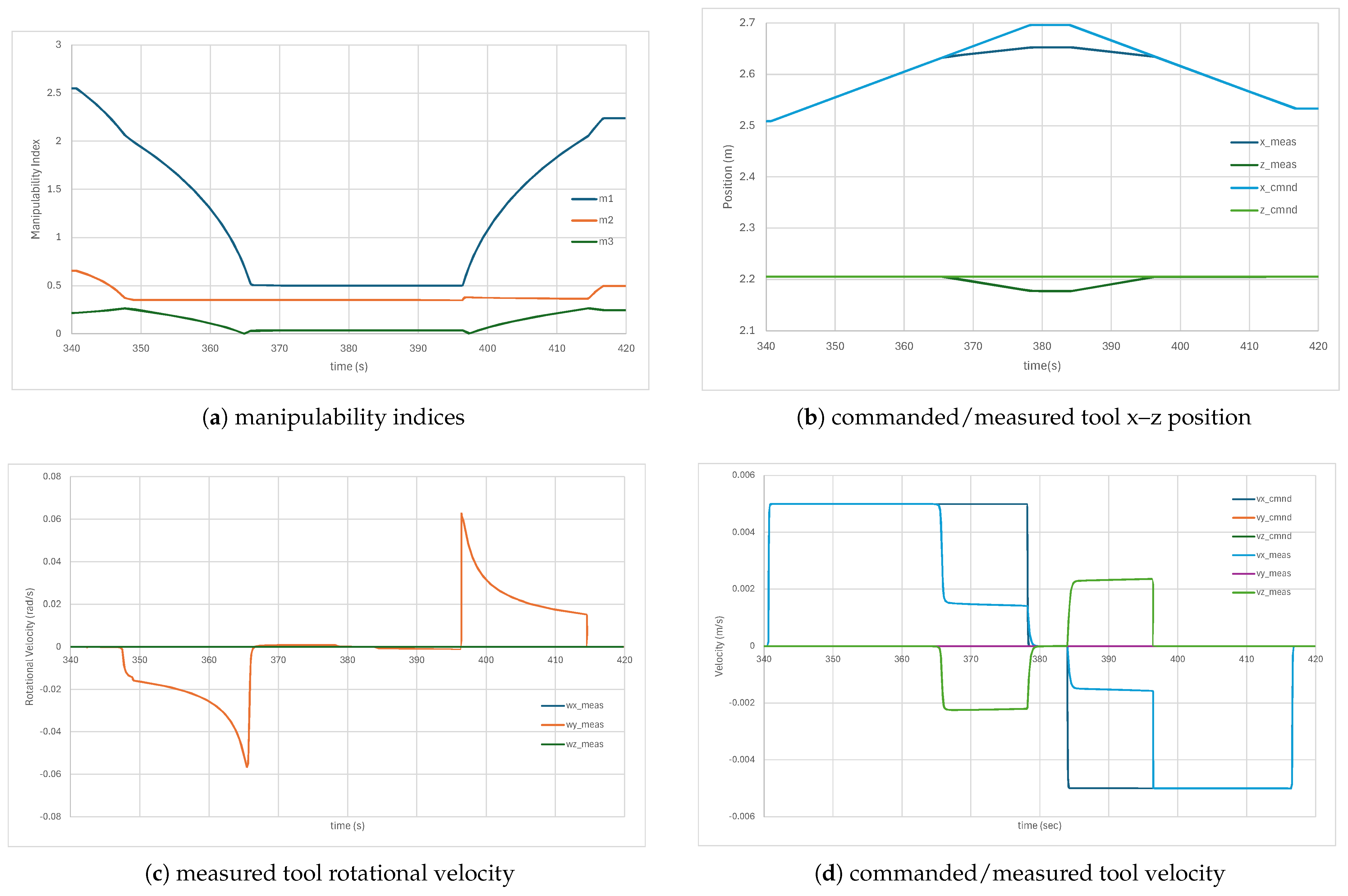
4.2. Elbow Pitch Singularity

The starting configuration for this simulation is $\theta ={[0,50,60,0,-20,0]}^{\circ }$ shown in Figure 9b with the elbow nearing its singular configuration of ${\theta }_3={78.99}^{\circ }$ and just outside the workspace boundary. In this configuration, both rotational manipulabilities are already within their transition boundaries of 0.70 and 0.30, respectively, as shown in Figure 11a. The results for the manipulabilities and tool positions/velocities are shown in Figure 11.

The tool was commanded to move at 0.5 cm/s in the $x_0$-direction, as seen in Figure 11b,d until the orientation error started building up just before 350 s. At this point, the Task 2 manipulability hits its threshold at 0.30 and the desired orientation can no longer be maintained as shown in the measured rotational velocity in Figure 11c.

At 365 s, the Task 1 manipulability boundary at ${\overline{m}}_1=0.5$ is reached and the tool $x_0$-$z_0$ position error builds up as seen in Figure 11b. The path is modified such that it now moves along the singularity surface and the tool never tries to penetrate the workspace boundary. At about 380 s, the commanded direction is reversed and the manipulator starts returning to a controllable state. The position error reduces to 0 m by 400 s, and the rotational error continues to unwind.

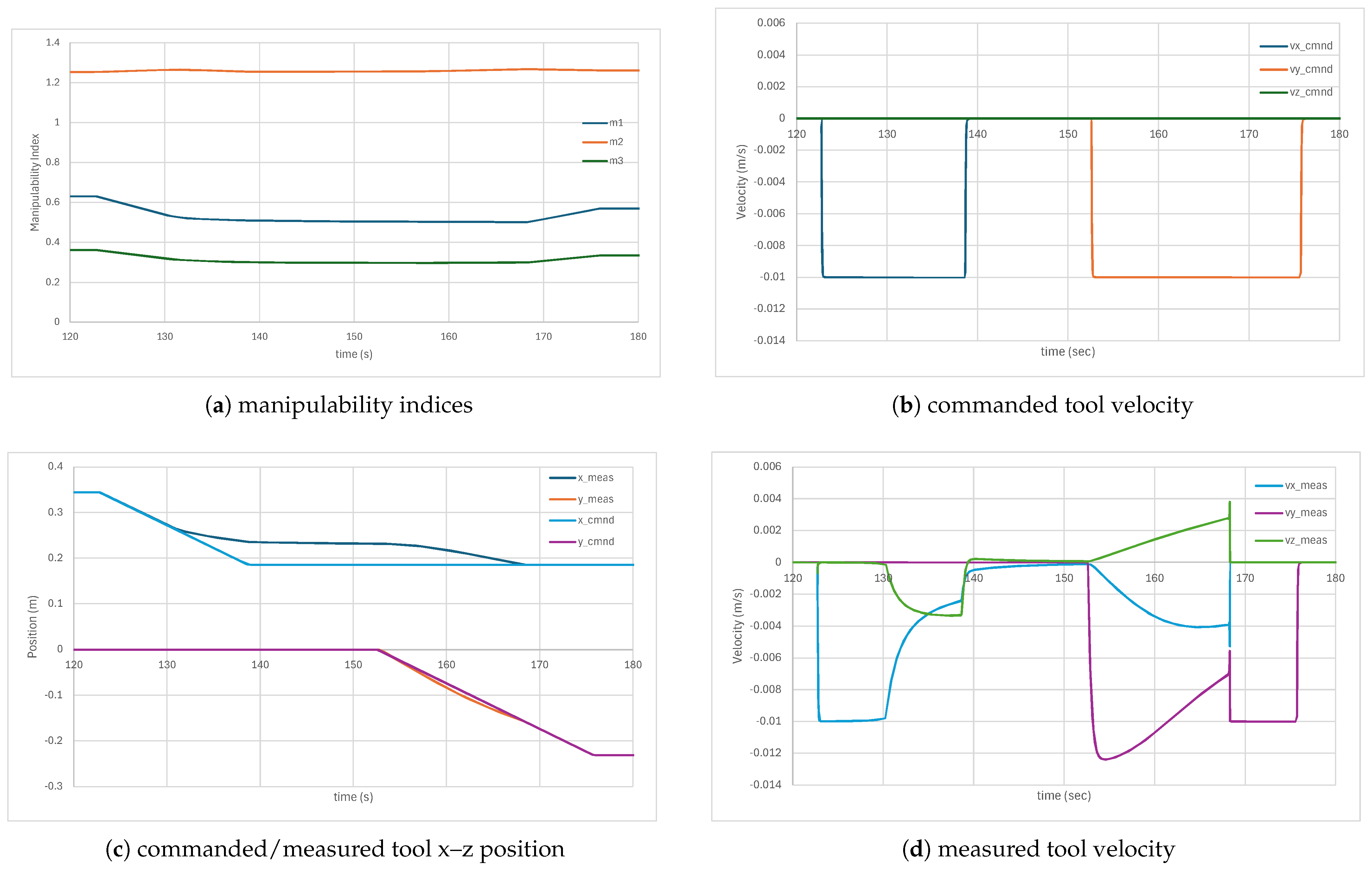
4.3. Wrist on Joint 1 Axis

The starting configuration for this simulation is $\theta ={[0,120,20,0,40,0]}^{\circ }$ shown in Figure 9c with wrist close to the joint 1 axis (note that ${\theta }_2=129.{238}^{\circ }$ would put it on the axis). Because the Task 1 manipulability bound is enforced, the wrist will not be able to pass overhead through the shoulder yaw axis. The results for the manipulabilities and tool positions/velocities are shown in Figure 12.

The tool velocity was commanded at 1 cm/s in the negative $x_0$-direction driving the wrist toward the $z_1$ axis which is coincident with base frame $z_0$-axis as seen in Figure 12b,c. Just after 130 s, the x-position begins to deviate from the commanded path as the Task 1 manipulability hits its threshold at 0.5 preventing the wrist from hitting the $z_0$-axis as seen in Figure 12a.

When the position error reaches 0.05 m just after 150 s, the x-velocity command is stopped, and the negative y-command of 0.5 cm/s is issued as seen in Figure 12b. This moves the tool away from the $z_0$-axis and singular configuration eventually increasing the Task 1 manipulability above its threshold of 0.5. By 170 s, the Task 1 manipulability rises above its threshold, and the x–z positions are able to follow the commanded values as seen in Figure 12c.

5. Conclusions

A new inverse kinematics approach was developed for a six-axis manipulator that partitions the operational space into three subtasks: (1) tool position, (2) tool orientation plane orthogonal to wrist singularity, and (3) tool orientation in singular direction. The subtasks were given a priority for maintaining the desired path when the inverse kinematics encounters singularity constraints. The Task Reconstruction (TR) method enables the robot to move along a singularity-free path for the first pair of tasks with priority given to tool translation. The third task corresponds to the singular direction caused by $0^{\circ }$ wrist pitch and is dropped in the singular region to allow the wrist pitch to pass through the singularity. The application of this approach was demonstrated on the Motoman MH250 six-axis manipulator on a robot simulator running at 500 Hz.

While the TPIK method is not new, it has not been used in this way for singularity handling in six-axis manipulators. The main contributions of this approach include: (a) prioritization of tool position over tool orientation at singularities, (b) partitioning of the operational workspace to allow passage of the wrist through its singularity while preserving tool translation, and (c) smooth operation at the workspace boundary. Simulations validated the task prioritization of tool position over tool orientation in singular regions, and they also demonstrated smooth transition of the wrist through gimbal lock. The prioritization of tool position is especially important when operating in close proximity of surfaces so as not to cause inadvertent collisions.

A couple of disadvantages of the TPIK approach are (a) increased computational load for singularity avoidance and (b) high velocities at the singularity boundary. The increased computations can be offset by placing position-dependent computations such as the manipulability gradients in a slower, position-dependent loop. Moreover, the use of Cholesky Decomposition (over Singular Value Decomposition) on reduced dimension partitioned Jacobians represent a significant cost savings. Peak velocities are typically encountered during transitions on and off the singularity boundary due to the proximity to the singularity, which may still cause the Jacobians to be ill-conditioned. If desired, peak velocity can be reduced by increasing the singularity distance threshold, at the expense of reduced workspace. Future work could incorporate an external joint velocity/acceleration limiting algorithm to reduce this effect [22].

The partitioned operational space scheme can also be extended to manipulators with kinematically redundancy, such as anthropomorphic arms with elbow swivel self-motion [23,24,25] and 7-DOF manipulators mounted to mobile-bases [14,26]. The methodology was also successfully applied to an 8-DOF powered-exoskeleton where the kinematics were split into four operational tasks to provide smoother and safer human operation [27]. In addition, this approach was extended to the 7-DOF Motoman SIA50D manipulator that used a third task to control the arm self-motion. A companion paper to the research described here is currently in progress.

References

1. Chang, K.S.; Khatib, O. Manipulator Control at Kinematic Singularities: A Dynamically Consistent Strategy. In Proceedings of the IEEE/RSJ International Conference on Intelligent Robots and Systems (IROS), Pittsburgh, PA, USA, 5–9 August 1995; Volume 3, pp. 3084–3088. [Google Scholar]
2. Wampler, C.W. Manipulator Inverse Kinematic Solutions Based on Vector Formulations and Damped Least-Squares Methods. IEEE Trans. Syst. Man Cybern. 1986, 16, 93–101. [Google Scholar] [CrossRef]
3. Nakamura, Y.; Hanafusa, H. Inverse Kinematic Solutions With Singularity Robustness for Robot Manipulator Control. ASME J. Dyn. Syst. Meas. Control 1986, 108, 163–171. [Google Scholar] [CrossRef]
4. Caccavale, F.; Chiaverini, S.; Siciliano, B. Second-Order Kinematic Control of Robot Manipulators with Jacobian Damped Least-Squares Inverse: Theory and Experiments. IEEE/ASME Trans. Mechatronics 1997, 2, 188–194. [Google Scholar] [CrossRef]
5. Chiaverini, S.; Siciliano, B.; Egeland, O. Review of the Damped Least-Squares Inverse Kinematics with Experiments on an Industrial Robot Manipulator. IEEE Trans. Control Syst. Technol. 1994, 2, 123–134. [Google Scholar] [CrossRef]
6. Chiaverini, S.; Egeland, O. A Solution to the Singularity Problem for Six-Joint Manipulators. In Proceedings of the IEEE International Conference on Robotics and Automation (ICRA), Cincinnati, OH, USA, 13–18 May 1990; pp. 644–649. [Google Scholar]
7. Oetomo, D.; Ang, M.; Lim, S.Y. Singularity Handling on Puma in Operational Space Formulation. In Proceedings of the International Symposium on Experimental Robotics: Experimental Robotics VII, Waikiki, HI, USA, 11–13 December 2000; Springer: Berlin/Heidelberg, Germany, 2000; pp. 491–500. [Google Scholar]
8. Leontjevs, V.; Flores, F.G.; López, J.; Ribickis, L.; Kecskeméthy, A. Singularity Avoidance by Virtual Redundant Axis and its Application to Large Base Motion Compensation of Serial Robots. In Proceedings of the 21st International Workshop on Robotics in Alpe-Adria-Danube (RAAD) Region, Napoli, Italy, 10–13 September 2012. [Google Scholar]
9. Flores, F.G.; Röttgermann, S.; Weber, B.; Kecskeméthy, A. Generalization of the Virtual Redundant Axis Method to Multiple Serial-Robot Singularities. In Proceedings of the ROMANSY 22—Robot Design, Dynamics and Control, Rennes, France, 25–28 June 2018; Arakelian, V., Wenger, P., Eds.; Springer: Cham, Switzerland, 2019; pp. 499–506. [Google Scholar] [CrossRef]
10. Moe, S.; Antonelli, G.; Teel, A.R.; Pettersen, K.Y.; Schrimpf, J. Set-Based Tasks within the Singularity-Robust Multiple Task-Priority Inverse Kinematics Framework: General Formulation, Stability Analysis, and Experimental Results. Front. Robot. AI 2016, 3, 16. [Google Scholar] [CrossRef]
11. Ginnante, A.; Simetti, E.; Caro, S.; Leborne, F. Task priority based design optimization of a kinematic redundant robot. Mech. Mach. Theory 2023, 187, 105374. [Google Scholar] [CrossRef]
12. Chiaverini, S. Singularity-Robust Task-Priority Redundancy Resolution for Real-time Kinematic Control of Robot Manipulators. IEEE Trans. Robot. Autom. 1997, 13, 398–410. [Google Scholar] [CrossRef]
13. Marani, G.; Kim, J.; Yuh, J.; Chung, W.K. Algorithmic Singularities Avoidance in Task-Priority Based Controller for Redundant Manipulators. In Proceedings of the IEEE/RSJ International Conference on Intelligent Robots and Systems (IROS), Las Vegas, NV, USA, 27 October–1 November 2003; pp. 3570–3574. [Google Scholar]
14. Marani, G.; Yuh, J. Introduction to Autonomous Manipulation—Case Study with an Underwater Robot, SAUVIM; Springer Tracts in Advanced Robotics; Springer: Berlin/Heidelberg, Germany, 2014; Volume 102. [Google Scholar] [CrossRef]
15. Nakamura, Y. Advanced Robotics: Redundancy and Optimization; Addison Wesley: Reading, MA, USA, 1991. [Google Scholar]
16. Siciliano, B.; Slotine, J.J. A general framework for managing multiple tasks in highly redundant robotic systems. In Proceedings of the 5th International Conference on Advanced Robotics, Pisa, Italy, 19–22 June 1991; Volume 2, pp. 1211–1216. [Google Scholar]
17. Baerlocher, P.; Boulic, R. Task-Priority Formulations for the Kinematic Control of Highly Redundant Articulated Structures. In Proceedings of the IEEE/RSJ International Conference on Intelligent Robots and Systems (IROS), Victoria, BC, Canada, 13–17 October 1998; pp. 323–329. [Google Scholar]
18. Yoshikawa, T. Manipulability of Robotic Mechanisms. Int. J. Robot. Res. 1985, 4, 3–9. [Google Scholar] [CrossRef]
19. Park, J. Analysis and Control of Kinematically Redundant Manipulators: An Approach Based on Kinematically Decoupled Joint Space Decomposition. Ph.D. Thesis, Pohang University of Science and Technology (POSTECH), Pohang-si, Republic of Korea, 1999. [Google Scholar]
20. Press, W.; Flannery, B.; Teukolsky, S.; Vetterling, W. Numerical Recipes in C: The Art of Scientific Computing, 2nd ed.; Cambridge University Press: Cambridge, UK, 1992. [Google Scholar]
21. Marani, G.; Kim, J.; Yuh, J.; Chung, W.K. A real-time approach for singularity avoidance in Resolved Motion Rate Control of Robotic Manipulators. In Proceedings of the IEEE International Conference on Robotics and Automation (ICRA), Washington, DC, USA, 11–15 May 2002; pp. 1973–1978. [Google Scholar]
22. Red, E.; Fielding, B. Predictive joint motion limiting in robotic applications. Robotica 2003, 21, 531–540. [Google Scholar] [CrossRef]
23. Seraji, H. Configuration Control of Redundant Manipulators: Theory and Implementation. IEEE Trans. Robot. Autom. 1989, 5, 472–490. [Google Scholar] [CrossRef]
24. Kreutz-Delgado, K.; Long, M.; Seraji, H. Kinematic Analysis of 7 DOF Manipulators. Int. J. Robot. Res. 1992, 11, 469–481. [Google Scholar] [CrossRef]
25. Cui, Z.; Pan, H.; Qian, D.; Peng, Y.; Han, Z. A Novel Inverse Kinematics Solution for a 7-DOF Humanoid Manipulator. In Proceedings of the IEEE International Conference on Mechatronics and Automation, Chengdu, China, 5–8 August 2012; pp. 2230–2234. [Google Scholar]
26. Simetti, E.; Casalino, G.; Wanderlingh, F.; Aicardi, M. Task priority control of underwater intervention systems: Theory and applications. Ocean Eng. 2018, 164, 40–54. [Google Scholar] [CrossRef]
27. Carignan, C.; Gribok, D.; Rappaport, T.; Condzal, N. Operational Space Formulation and Inverse Kinematics for an Arm Exoskeleton with Scapula Rotation. In Proceedings of the IEEE/RSJ International Conference on Intelligent Robots and Systems (IROS), Las Vegas, NV, USA, 25–29 October 2020; pp. 3389–3396. [Google Scholar] [CrossRef]
28. Craig, J.J. Introduction to Robotics: Mechanics and Control, 4th ed.; Pearson Education: Hoboken, NJ, USA, 2017. [Google Scholar]
29. Sciavicco, L.; Siciliano, B. Modeling and Control of Robot Manipulators, 2nd ed.; Springer: London, UK, 2000. [Google Scholar]
30. Konietschke, R.; Hirzinger, G.; Yan, Y. All singularities of the 9-DOF DLR medical robot setup for minimally invasive applications. In Proceedings of the Advances in Robot Kinematics: Mechanisms and Motion, Ljubljana, Slovenia, 25–29 June 2006; Springer: Dordrecht, The Netherlands; pp. 193–200. [Google Scholar]
Figure 1. Examples of six-axis industrial robots with a roll-pitch-roll wrist.
Robotics 14 00060 g001
Figure 2. Schematic of roll-pitch-roll wrist frequently found on industrial robots.
Robotics 14 00060 g002
Figure 3. Joint Position Solver Block Diagram.
Robotics 14 00060 g003
Figure 4. Task priority inverse kinematics for three tasks.
Robotics 14 00060 g004
Figure 5. Task projection is used to reconstruct the path around a singularity.
Robotics 14 00060 g005
Figure 6. Prioritized decomposition of three tasks by velocity solver.
Robotics 14 00060 g006
Figure 7. Three-step process used for task decomposition.
Robotics 14 00060 g007
Figure 8. Task priority inverse kinematics embedded with iterative position solver.
Robotics 14 00060 g008
Figure 9. Starting configurations for simulations (axes: x—red, y—green, z—blue).
Robotics 14 00060 g009
Figure 10. Simulation results near 0 wrist pitch.
Robotics 14 00060 g010
Figure 11. Simulation results for elbow pitch singularity near workspace boundary.
Robotics 14 00060 g011
Figure 12. Simulation results for wrist on shoulder yaw axis.
Robotics 14 00060 g012
Disclaimer/Publisher’s Note: The statements, opinions and data contained in all publications are solely those of the individual author(s) and contributor(s) and not of MDPI and/or the editor(s). MDPI and/or the editor(s) disclaim responsibility for any injury to people or property resulting from any ideas, methods, instructions or products referred to in the content.