Singular Configuration Analysis of Modular-Driven 4- and 6-DoF Parallel Topology Robots

Abstract

The number of applications of parallel topology robots in industry is growing, and the interest of academics in finding new solutions and applications to implement such mechanisms is present all over the world. Industrywide, the most commonly used motion types need four- and six-degrees-of-freedom (DoF) robots. While there are commercial variants from different robot vendors, this study offers new alternatives to these. Based on Lie algebra synthesis, symmetrical parallel structures are identified, according to certain rules. Implementing 2-DoF actuation modules, the number of robot limbs is reduced compared to existing commercial robot structures. In terms of the applicability of a parallel mechanism (also concerning the control algorithm), it is important to determine singular configurations. Therefore, in addition to the kinematic schematics of the newly proposed mechanisms, their singular configurations are also discussed. Based on some dimensional simplifications (without a loss of generality), the conditions for the singular configurations are enumerated for the presented parallel topology robots with symmetrical kinematic chains. Finally, a comparison of the proposed mechanism is presented, considering its singular configurations.

1. Introduction

The need for robotization in industry is present, typically involving the implementation of serial and parallel topology robots. While the topological study of serial robots is straightforward, the complexity of their parallel counterparts continues to intrigue academics conducting industrial research. Lower-degree-of-freedom mechanisms, which are well suited for specific tasks, are often preferred due to their architectural simplicity, ease of mathematical modeling and control, and, importantly, their cost-effectiveness. According to the International Federation of Robotics, as cited by Balluff Inc. [1], the second-most widely used robot type is the SCARA type, which has a market share of approximately 15%, with a 5–10% per year growth rate. Based on this, it can be stated that the need for 4-degrees-of-freedom (DoF) robots in various industry sectors is real. The same source notes the 5% market share of Delta-type robots (with a 3–5% per year growth rate), which includes 3-, 4-, and 6-DoF robots. It is obvious that the dynamic properties are better in the case of 4-DoF Delta robots compared to their SCARA counterparts, but the workspace limitations of Delta robots hinder their widespread use. As such, various authors have sought to design a parallel and symmetrical topology 4-DoF robot by using Schoenflies motion generators as kinematic limbs [2,3,4,5,6,7,8]. Citing the same report [1], the largest market share (≈60%) is held by 6-DoF articulated robots with serial topologies. In the case of these all-purpose robots, we may observe the same advantages and drawbacks as 6-DoF parallel topology robots, i.e., bigger workspaces but poor dynamic properties. This contrast fuels research to find new parallel topology robots for optimized implementation.

The 6-DOF parallel mechanism, introduced by Stewart and Gough, has undergone extensive exploration since its inception, revealing various aspects of the mechanism and its applications [1,2]. Over the past few decades, significant attention has been devoted to studying 6-DOF parallel mechanisms [9,10,11,12,13,14,15,16,17,18], including their kinematics, dynamics, singularities, errors, and workspaces, as well as special topology robots [19,20,21] and lower-mobility mechanisms [22,23,24,25,26,27], with a notable focus on Schoenflies motion generator mechanisms [2,3,4,5,7,8,28,29,30,31,32,33,34,35,36,37,38,39,40,41]. Using the new driving module and based on synthesis studies in the literature, new structures are constantly being introduced and analyzed.

Notable contributions to the synthesis of new kinematic structures were made by Earl and Rooney, who introduced a component-based methodology to construct and modify manipulator designs [42]. Noteworthy further research includes Hunt’s analysis of manipulators using screw theory [43], Tsai’s application of a systematic methodology [44], and Angeles’ discussion of the structural synthesis of parallel robots using mathematical group theory [45]. More recently, Shen proposed a systematic synthesis methodology for 6-DOF kinematic structures, identifying 29 distinct parallel structures [46]. A framework and brief review of this type of synthesis were authored by Meng et al. [47].

Tsai [44] defines a parallel manipulator as symmetrical if the number of limbs equals the number of degrees of freedom of the moving platform. However, in the case of double-actuated kinematic chains (featuring two actuated joints on one kinematic chain), this symmetry condition may be disregarded. The base and moving platform’s serial kinematic chains must have the same topology for symmetrical mechanisms to work. This study will present some kinematic structures according to the above-mentioned criteria; it does not represent a systematic discussion of 4- and 6-DoF structures. Furthermore, a comprehensive study of the presented kinematic structures is beyond the scope of this study; however, a singular configuration analysis of such parallel topology robots is carried out using Jacobian matrix analysis. Highlighting kinematic equations in parametrized form for the newly introduced structures gives rise to the possibility of developing adapted structures for specific technological processes. This form of study has gained broad acceptance in different robotic fields [23,40,48,49,50,51,52,53,54,55,56].

2. Kinematics of 2-DoF Actuation Module

The authors of [57,58] briefly described modular manipulators ranging from 2- to 4-DoF mechanisms. The basis of these manipulators was a 2-DoF, double-actuated module, the output of which achieves controlled translational and rotational motion [59]. These movements are accomplished via two motorized axes, as shown in Figure 1. Angular displacements $q_1$ and $q_2$ serve as the input of the module, which are induced by the two drives (equipped with toothed belt pulleys with radius r) on the left and right sides of the module. They pull a toothed belt, which is led through other pulleys, as depicted. The central piece of the module is a slider, containing two pulleys with a radius of R. Using this setup, if the drives are rotating in the same direction with the same angular speed, the rotation of the spindle axis (denoted by θ) occurs. On the other hand, if they are rotating in opposite directions with the same angular speed, in addition to the rotation of the spindle, the slider undergoes linear displacement (denoted by d). The relationship between the input and output parameters is straightforward, because the geometric parameters of the module do not depend on time, as shown below:

$$\left[\begin{array}{c}d\\ \theta \end{array}\right]=\left[\begin{array}{cc}{\displaystyle \frac{-r}{2}}& {\displaystyle \frac{r}{2}}\\ {\displaystyle \frac{-r}{2R}}& {\displaystyle \frac{-r}{2R}}\end{array}\right]\left[\begin{array}{c}{q}_1\\ q_2\end{array}\right],\mathrm{and}$$

(1)

$$\left[\begin{array}{c}\dot{d}\\ \dot{\theta }\end{array}\right]=\left[\begin{array}{cc}{\displaystyle \frac{-r}{2}}& {\displaystyle \frac{r}{2}}\\ {\displaystyle \frac{-r}{2R}}& {\displaystyle \frac{-r}{2R}}\end{array}\right]\left[\begin{array}{c}{\dot{q}}_1\\ {\dot{q}}_2\end{array}\right]$$

(2)

The working principle of the module is described in [60], which verifies that the presented setup may be used as a 2-DoF actuation unit in a kinematic chain of parallel topology mechanisms. Typically, in these systems, each kinematic chain has a single-actuated joint to comply with the criterion that specifies that the number of chains must equal the robot’s DoF. When each kinematic chain has two actuated joints, the number of kinematic chains may be halved. Adhering to this principle, the present study proposes some mechanisms in which the lower pair of joints (translational and rotational joints, in that particular order) is replaced by the double-actuated module from Figure 1. There are several advantages of the completion of mechanisms and the reduction in the number of kinematic chains in the robot mechanism by half. On the one hand, it means less mass to move; therefore, it results in better dynamic properties. On the other hand, having fewer kinematic chains decreases the likelihood of self-collision, which may result in a bigger workspace and reduced singular configurations.

Industrial tasks that require 4-DoF and 6-DoF robots (e.g. pick-and-place, packaging, etc. [1]) can take advantage of the parallel topology based on the double-actuated modules seen in the previous paragraph. In the forthcoming sections, 4-DoF and 6-DoF mechanisms containing two and three of the mechanisms, respectively, from Figure 1 as actuation units will be investigated.

In the case of 4-DoF mechanisms, the robot parameter vector can be written as $\mathit{q}={\left[\begin{array}{cccc}{q}_1& q_2& q_3& q_4\end{array}\right]}^T$; therefore, the robot joint velocities are represented by the vector $\dot{\mathit{q}}={\left[\begin{array}{cccc}{\dot{q}}_1& {\dot{q}}_2& {\dot{q}}_3& {\dot{q}}_4\end{array}\right]}^T$. To obtain the kinematic relation between the four input and four output parameters, Equation (2) must be doubled, as follows:

$$\left[\begin{array}{c}{\dot{d}}_1\\ {\dot{\theta }}_1\\ {\dot{d}}_2\\ {\dot{\theta }}_2\end{array}\right]=\left[\begin{array}{cccc}-{\displaystyle \frac{r}{2}}& {\displaystyle \frac{r}{2}}& 0& 0\\ -{\displaystyle \frac{r}{2R}}& -{\displaystyle \frac{r}{2R}}& 0& 0\\ 0& 0& -{\displaystyle \frac{r}{2}}& {\displaystyle \frac{r}{2}}\\ 0& 0& -{\displaystyle \frac{r}{2R}}& -{\displaystyle \frac{r}{2R}}\end{array}\right]·\left[\begin{array}{c}{\dot{q}}_1\\ {\dot{q}}_2\\ {\dot{q}}_3\\ {\dot{q}}_4\end{array}\right]=J_{4m}\left[\begin{array}{c}{\dot{q}}_1\\ {\dot{q}}_2\\ {\dot{q}}_3\\ {\dot{q}}_4\end{array}\right]⟹{\dot{\mathit{q}}}_{par}=J_{4m}\dot{\mathit{q}},$$

(3)

where the ${\left[\begin{array}{cccc}{\dot{d}}_1& {\dot{\theta }}_1& {\dot{d}}_2& {\dot{\theta }}_2\end{array}\right]}^T$ vector represents the output velocities of the two actuated modules, and $J_{4m}$ denotes the Jacobian matrix of the modules.

It must be noted that the determinants of the Jacobian matrices always have a non-zero value ($det\left(J_{4m}\right)=r^4/4R^2$ and $det\left(J_{4m}^{-1}\right)=4R^2/r^4$), because the radius of the pulleys cannot be zero. Therefore, the inverse matrix may be calculated and used in the inverse kinematic relation, as follows:

$$\left[\begin{array}{c}{\dot{q}}_1\\ {\dot{q}}_2\\ {\dot{q}}_3\\ {\dot{q}}_4\end{array}\right]=\left[\begin{array}{cccc}-{\displaystyle \frac{1}{r}}& -{\displaystyle \frac{R}{r}}& 0& 0\\ {\displaystyle \frac{1}{r}}& -{\displaystyle \frac{R}{r}}& 0& 0\\ 0& 0& -{\displaystyle \frac{1}{r}}& -{\displaystyle \frac{R}{r}}\\ 0& 0& {\displaystyle \frac{1}{r}}& -{\displaystyle \frac{R}{r}}\end{array}\right]\left[\begin{array}{c}{\dot{d}}_1\\ {\dot{\theta }}_1\\ {\dot{d}}_2\\ {\dot{\theta }}_2\end{array}\right]=J_{4m}^{-1}\left[\begin{array}{c}{\dot{d}}_1\\ {\dot{\theta }}_1\\ {\dot{d}}_2\\ {\dot{\theta }}_2\end{array}\right]⟹\dot{\mathit{q}}=J_{4m}^{-1}{\dot{\mathit{q}}}_{par},$$

(4)

The same methodology applies in the case of 6-DoF robots, if the actuation of the robot is performed by the mechanism from Figure 1. In this case, the robot mechanism features three pairs of input parameters for every kinematic chain, consisting of parameters $d_i$ and ${\theta }_i$ $\left(i=1,2,3\right)$. The assembly of the Jacobian matrix and its inverse, based on Equation (2), is defined as follows:

$$\left[\begin{array}{c}{\dot{d}}_1\\ {\dot{\theta }}_1\\ {\dot{d}}_2\\ {\dot{\theta }}_2\\ {\dot{d}}_3\\ {\dot{\theta }}_3\end{array}\right]=\left[\begin{array}{cccccc}-{\displaystyle \frac{r}{2}}& {\displaystyle \frac{r}{2}}& 0& 0& 0& 0\\ -{\displaystyle \frac{r}{2R}}& -{\displaystyle \frac{r}{2R}}& 0& 0& 0& 0\\ 0& 0& -{\displaystyle \frac{r}{2}}& {\displaystyle \frac{r}{2}}& 0& 0\\ 0& 0& -{\displaystyle \frac{r}{2R}}& -{\displaystyle \frac{r}{2R}}& 0& 0\\ 0& 0& 0& 0& -{\displaystyle \frac{r}{2}}& {\displaystyle \frac{r}{2}}\\ 0& 0& 0& 0& -{\displaystyle \frac{r}{2R}}& -{\displaystyle \frac{r}{2R}}\end{array}\right]\left[\begin{array}{c}\begin{array}{c}{\dot{q}}_1\\ {\dot{q}}_2\\ {\dot{q}}_3\\ {\dot{q}}_4\\ {\dot{q}}_5\\ {\dot{q}}_6\end{array}\end{array}\right]=J_{6m}\left[\begin{array}{c}{\dot{q}}_1\\ {\dot{q}}_2\\ {\dot{q}}_3\\ {\dot{q}}_4\\ {\dot{q}}_5\\ {\dot{q}}_6\end{array}\right]⟹{\dot{\mathit{q}}}_{par}=J_{6m}\dot{\mathit{q}},$$

(5)

$$\left[\begin{array}{c}{\dot{q}}_1\\ {\dot{q}}_2\\ {\dot{q}}_3\\ {\dot{q}}_4\\ {\dot{q}}_5\\ {\dot{q}}_6\end{array}\right]=\left[\begin{array}{cccccc}-{\displaystyle \frac{1}{r}}& -{\displaystyle \frac{R}{r}}& 0& 0& 0& 0\\ {\displaystyle \frac{1}{r}}& -{\displaystyle \frac{R}{r}}& 0& 0& 0& 0\\ 0& 0& -{\displaystyle \frac{1}{r}}& -{\displaystyle \frac{R}{r}}& 0& 0\\ 0& 0& {\displaystyle \frac{1}{r}}& -{\displaystyle \frac{R}{r}}& 0& 0\\ 0& 0& 0& 0& -{\displaystyle \frac{1}{r}}& -{\displaystyle \frac{R}{r}}\\ 0& 0& 0& 0& {\displaystyle \frac{1}{r}}& -{\displaystyle \frac{R}{r}}\end{array}\right]\left[\begin{array}{c}{\dot{d}}_1\\ {\dot{\theta }}_1\\ {\dot{d}}_2\\ {\dot{\theta }}_2\\ {\dot{d}}_3\\ {\dot{\theta }}_3\end{array}\right]=J_{6m}^{-1}\left[\begin{array}{c}{\dot{d}}_1\\ {\dot{\theta }}_1\\ {\dot{d}}_2\\ {\dot{\theta }}_2\\ {\dot{d}}_3\\ {\dot{\theta }}_3\end{array}\right]⟹\dot{\mathit{q}}=J_{6m}^{-1}{\dot{\mathit{q}}}_{par}.$$

(6)

The inversion of the Jacobian matrix may always be performed due to its non-zero determinant, as in the preceding situation. ($det\left(J_{6m}\right)=r^6/8R^3$). It may be concluded that the constant Jacobian matrices from Equations (3) and (5) represent transmission ratios, so that the use of the actuation modules will not influence the modeling methodology of the proposed mechanisms.

Figure 1 illustrates that the spindle axis direction is perpendicular to the slider’s translation direction, allowing for subsequent translational and rotational joints, whose axes are perpendicular, to be replaced by the module. But allowing an expansion of the spindle axis by a bevel gear coupling, its rotation can be redirected in any direction (Figure 1b–d). For instance, the circumstance of parallel directions of output rotation and slider translation may be achieved.

3. Serial Chain Motion Generators

The enumeration of those serial topology chains, which enable the spatial motion (three translations and three rotations), is greatly simplified by using the Lie group of rigid body displacement, as introduced by Hervé [61], presented by Selig [62] and synthesized by Ye and Li [27]. According to them, if the subsets of possible displacements generated by each limb of a parallel manipulator are a Lie subgroup, then the intersection set is also a Lie subgroup of the mobile platform [27]:

$$\left\{M\right\}={\cap }_{i=1}^n\left\{L_{\mathrm{i}}\right\}.$$

(7)

According to this statement, if the platform undergoes the spatial motion ($\left\{M\right\}=\left\{D\right\}$), each chain must allow the three translations and three rotations. According to

Table 1. List of displacements in Lie subgroups [61].

Lie Subgroup	Description of the Subgroup
{E}	identity
$\left\{T\right(\mathit{u}\left)\right\}$	translation parallel with the u vector
$\left\{R\right(N,\mathit{u}\left)\right\}$	rotation around the axis determined by N and u
$\left\{H\right(N,\mathit{u},p\left)\right\}$	helical motions with axis (N,u) and the pitch p
$\left\{T\right(Pl\left)\right\}$	translations parallel with the Pl plane
$\left\{C\right(N,\mathit{u}\left)\right\}$	cylindrical motions along an axis (N,u)
$\left\{T\right\}$	spatial translations
$\left\{G\right(\mathit{u}\left)\right\}$	planar gliding motions perpendicular to u
$\left\{S\right(N\left)\right\}$	spherical motions about point N
$\left\{X\right(\mathit{u}\left)\right\}$	Schoenflies motions
$\left\{D\right\}$	general rigid body motions or displacements

(as presented in [61]), {D} denotes the general rigid body motions of the 6-DoF mobile platform. Based on the Lie group theory, {L_i} denotes the displacement Lie subgroup of the ith chain. If a 6-DoF mechanism has only three, yet double-actuated kinematic chains (n = 3), a true relation (7) is given by:

$$\left\{L_1\right\}=\left\{L_2\right\}=\left\{L_3\right\}=\left\{D\right\}.$$

(8)

For a simple mechanical structure, a symmetric kinematic chain architecture must be considered for a parallel topology robot, as this requires identical sets of parts.

Based on group theory, it can be stated that when $\forall N\mathrm{a}\mathrm{n}\mathrm{d}\mathit{v}\perp \mathit{w}\perp \mathit{u}$, the following relationship also applies:

$$\left\{L_i\right\}=\left\{D\right\}=\left\{T\right\}\left\{S\left(N\right)\right\}=\left\{T\left(\mathit{u}\right)\right\}\left\{T\left(\mathit{v}\right)\right\}\left\{T\left(\mathit{w}\right)\right\}\left\{R\left(N,\mathit{u}\right)\right\}\left\{R\left(N,\mathit{v}\right)\right\}\left\{R\left(N,\mathit{w}\right)\right\}.$$

Taking into consideration the properties of the Lie subgroups, the right side of Equation (3) may be grouped to have Lie subgroups, which can be realized with the proposed mechanisms.

From Equation (5), it can be observed that the presented 6 DoFs may be divided into two groups: one consisting of the three translations that allow for spatial positioning, and another one with the three rotations, which are responsible for the orientation of the mechanism. Taking this into account, the various Lie subgroups from

Table 2. Variation in Lie subgroups in order to realize the 6 DoF $\left\{L_i\right\}$.

Case	Lie Subgroup for Spatial Positioning	Lie Subgroup for Spatial Orientation	Observations
(a)	$\left\{T\left(\mathit{u}\right)\right\}\left\{T\left(\mathit{v}\right)\right\}\left\{T\left(\mathit{w}\right)\right\}$	$\left\{R\left(N,\mathit{u}\right)\right\}\left\{R\left(N,\mathit{v}\right)\right\}\left\{R\left(N,\mathit{w}\right)\right\}$	$\forall N,\mathit{u}\perp \mathit{v}\perp \mathit{w}$
(b)	$\left\{R\left(A,\mathit{u}\right)\right\}\left\{T\left(\mathit{u}\right)\right\}\left\{T\left(\mathit{v}\right)\right\}$	$\left\{R\left(N,\mathit{u}\right)\right\}\left\{R\left(N,\mathit{v}\right)\right\}\left\{R\left(N,\mathit{w}\right)\right\}$	$\forall N,A,\mathit{u}\perp \mathit{v}\perp \mathit{w}$
(c)	$\left\{R\left(A,\mathit{u}\right)\right\}\left\{T\left(\mathit{u}\right)\right\}\left\{R\left(C,\mathit{w}\right)\right\}$	$\left\{R\left(N,\mathit{u}\right)\right\}\left\{R\left(N,\mathit{v}\right)\right\}\left\{R\left(N,\mathit{w}\right)\right\}$	$\forall N,A,C,\mathit{u}\perp \mathit{v}\perp \mathit{w}$
(d)	$\left\{R\left(A,\mathit{u}\right)\right\}\left\{T\left(\mathit{u}\right)\right\}\left\{R\left(C,\mathit{v}\right)\right\}$	$\left\{H\right(N,\mathit{v},p\left)\right\}\left\{R\left(N,\mathit{u}\right)\right\}\left\{R\left(N,\mathit{w}\right)\right\}$	$\forall N,A,C,\mathit{u}\perp \mathit{v}\perp \mathit{w}$
(e)	$\left\{R\left(A,\mathit{u}\right)\right\}\left\{R\left(A,\mathit{v}\right)\right\}\left\{T\left(\mathit{w}\right)\right\}$	$\left\{R\left(N,\mathit{u}\right)\right\}\left\{R\left(N,\mathit{v}\right)\right\}\left\{R\left(N,\mathit{w}\right)\right\}$	$\forall N,A,\mathit{u}\perp \mathit{v}\perp \mathit{w}$

realize the desired degrees-of-freedom mechanisms. Thereupon, the spatial orientation can only be realized by rotation, while the spatial positioning may involve translations and/or rotations. To describe the spatial motion of a point, the combination of the translational and rotational subgroups from Table 2 should be used. In accord with this, case (a) is based on the orthogonal, (b)–(d) are based on cylindrical and (e) is based on spherical coordinate system parameters.

Hence, a primary issue related to parallel topology mechanisms and robots is the size and homogeneity of the workspace. One of the goals of this study is to identify the solutions that can be implemented to maximize the aforementioned features. To select the subgroups suitable for implementation in a parallel topology robot with symmetric kinematic chains, the following features are considered:

• The workspace of the robot;
• Usability of the 2-DoF actuation module;
• The position of the actuated joints relative to the kinematic chain.

The use of the 2-DoF module (having one translational and one rotational degree of freedom) prioritizes those cases in which both subgroups of $\left\{T\left(\dots \right)\right\}$ and $\left\{R\left(\dots \right)\right\}$ are present. Although a translational DoF can be realized with multiple rotational joints as well, this involves an additional mechanism, which would lead to an increase in the mass of the kinematic chain and would negatively influence the dynamics of the robot. For this reason, case (a) is out of the scope of this study.

Based on cases (b)–(e) from Table 2, 12 variants shown in Figure 2 may be considered for further investigation, considering that in every variant, there is a translational joint that is followed by a rotational one.

Thus, 8 of the 12 variants can be excluded from the investigation forthwith, as they do not adhere to at least one of the following criteria:

• Because the successive translational and rotational joints are supposed to be realized with the proposed 2-DoF actuation module, it is preferred that the third, i.e., the passive joint in the kinematic chains, is found at the end of a linkage. This ensures that the actuation units are linked to the robot base, so the moving mass may be reduced, which has a positive influence on the dynamics of the robot. Therefore, the variants (b1), (c3) and (e3) are not discussed further.
• The first joint in variant (b4) is a passive rotational one, but since its axis is parallel with that of the next active translational joint, a particular case emerges when the first two axes are coincident (zero distance between the axes). This could make it suitable for implementation because a good statically balanced mechanism may be constructed. But, as previously stated, the second active translational joint may not be replaced with active rotational joints due to additional mass reasons, so the (b4) variant is not considered for further investigation.
• Variants (b2) and (b3) are excluded because they feature a translational passive joint as the third joint in the linkage. This configuration is considered unfit for implementation in a symmetrical robot mechanism, as it will lead to excessively high internal forces acting perpendicularly to the axis of the translational joint. This will induce an over-dimensioning of the 2-DoF actuation unit, contrary to other variants, so the modular approach to the potential physical realization will be compromised. For that reason, variants (b2) and (b3) are omitted in further research.
• Variants (c2) and (e2) can be considered as special cases; as with specific geometrical dimensioning, they could be considered as planar mechanisms. Because of this, subsequent research will be carried out concerning them; hence, they are not included in this study.

This means that variants (c1), (d1), (d2) and (e1) are prone to be subjected to further investigations regarding the kinematics of 6-DoF robot mechanisms that feature symmetrical build-up.

The same logic must be applied in the case of 4-DoF robot structure design involving the double-actuation modules. Recalling Equation (7), new equalities must be defined based on Equations (7) and (8): $\left\{M\right\}=\left\{X\left(\mathit{u}\right)\right\}$ refers to the Schoenflies motion Lie subgroup, and $\left\{L_i\right\}=\left\{L_i^x\right\}$ refers to a new displacement Lie subgroup of the ith limb of the structure. For the 4-DoF mechanisms, two kinematic chains (n = 2) will be considered, $\mathit{u}$ as follows:

$$\left\{L_1^{\mathrm{x}}\right\}\cap \left\{L_2^{\mathrm{x}}\right\}=\left\{X\left(\mathit{u}\right)\right\},$$

(9)

$$\left\{L_1^{\mathrm{x}}\right\}=\left\{L_2^{\mathrm{x}}\right\}=\left\{X\left(\mathit{u}\right)\right\},$$

(10)

where it turns out that $\left\{L_i^x\right\}$ must be the displacement Lie subgroup of the ith limb realizing the Schoenflies motion. The synthesis of primitive Schoenflies motion generators has been made by Ch.-Ch. Leea and J. M. Hervé [8], so their work is the point of departure in our research. Taking into account the constraints for the joint types caused by the use of the 2-DoF actuation module, two variants were selected from [8] for further investigation (Figure 3). To be consistent with the Lie algebra notations (used in Table 1), the translational joint will be denoted by T, the rotational joint will be denoted by R, and the helical joint will be denoted by H. In addition to those notations, the universal joint will be denoted by U. Using the above notations, the selected Schoenflie motion generators are written as TRRH and TTTH.

4. Kinematic Analysis of 4-DoF Mechanisms Using Modular Actuation

Based on the mechanisms shown in Figure 3, three parallel topology robot structures that have 4 DoF realized through two kinematic chains are proposed. This section will present the kinematic analysis of the mechanisms by constructing their respective Jacobian matrix, which emphasizes the relation between the change in robot parameters (represented by the vector of joint velocities $\dot{\mathit{q}}={\left[\begin{array}{cccc}{\dot{q}}_1& {\dot{q}}_2& {\dot{q}}_3& {\dot{q}}_4\end{array}\right]}^T$) and the velocity of the tool center point (TCP) P (represented by the end effector velocities vector ${}^0\dot{\mathit{X}}={\left[\begin{array}{cccc}{\dot{x}}_P& {\dot{y}}_P& {\dot{z}}_P& {\dot{\beta }}_P\end{array}\right]}^T$).

4.1. The 2TRRH Robot Kinematics

The proposed architecture for the 2TRRH robot is presented in Figure 4. The topology of the robot is defined by the two TRRH Schoenflies motion generators, and the mechanism is closed by the $C_1^{\prime }{C}_2^{\prime }P$ screw. Using this setup, the spatial positioning of the point P and the horizontal rotation of the screw are described with the $d_1,d_2,{\theta }_1$, and ${\theta }_2$ controlled geometrical parameters. It is important to highlight that a particular setup can be derived from Figure 4a by introducing $p_2=0\mathrm{m}\mathrm{m}$. In this case, the $C_2^{\prime }$ helical joint is transformed into a rotational joint, allowing for simplified mathematical modeling (and, later, control) without altering the presented degrees of freedom of the point P. To simplify the annotation, the $p=p_1\ne 0$ convention is used. Other geometrical parameters are $B_1{C}_1=B_2{C}_2=h\left[\mathrm{mm}\right]$, $C_1{C}_1^{\prime }=C_2{C}_2^{\prime }=l\left[\mathrm{mm}\right]$ and $C_2^{\prime }P=d_p\left[\mathrm{mm}\right]$. The notations $s\alpha$, $s\beta$, and $s\gamma$ are being used to denote the sine, and $c\alpha$, $c\beta$ and $c\gamma$ are being used to denote the cosine of the angles $\alpha$, $\beta$ and $\gamma$.

Considering the notations from Figure 4, the inverse geometry relations for the two translational parameters are established, as follows:

$$d_2=y_P+d_P,$$

(11)

$$d_2-d_1={\displaystyle \frac{p}{2\pi }}{\beta }_P\Rightarrow d_1=d_2-{\displaystyle \frac{p}{2\pi }}{\beta }_P=y_P-d_P-{\displaystyle \frac{p}{2\pi }}{\beta }_P,$$

(12)

where p stands for the pitch of the screw in [mm] and ${\beta }_P$ denotes the rotation of the $C_1^{\prime }{C}_2^{\prime }P$ screw, expressed in radians.

Because of the symmetrical structure of the mechanism, the relation between the general parameters of point P and the ${\theta }_i$ parameters ($i\in \{1,2\}$) is given by the following equations:

$${\left(x_P-x_{Ci}\right)}^2+{\left(z_P-z_{Ci}\right)}^2-l^2=0,$$

(13)

$${\left(x_P-x_{Bi}-h\mathrm{c}{\theta }_i\right)}^2+{\left(z_P-h\mathrm{s}{\theta }_i\right)}^2-l^2=0,$$

(14)

where l is the length of $B_i{C}_i$, and h is the length of $C_i{C}_i^{\prime }$.

The time derivative Equations (11), (12), and (14) will be as follows:

$${\dot{d}}_1={\dot{y}}_P-{\displaystyle \frac{p}{2\pi }}{\dot{\beta }}_P,$$

(15)

$${\dot{d}}_2={\dot{y}}_P,$$

(16)

$$2\left(x_P-x_{Bi}-h\mathrm{c}{\theta }_i\right)\left({\dot{x}}_P+h\mathrm{s}{\theta }_i{\dot{\theta }}_i\right)+2\left(z_P-h\mathrm{s}{\theta }_i\right)\left({\dot{z}}_P-h\mathrm{c}{\theta }_i{\dot{\theta }}_i\right)=0.$$

(17)

Rearranging Equation (17), the final form becomes as follows:

$$\begin{gathered} 2h\left[s{\theta }_i\left(x_P-x_{Bi}-h\mathrm{c}{\theta }_i\right)+c{\theta }_i\left(z_P-h\mathrm{s}{\theta }_i\right)\right]{\dot{\theta }}_i=-2\left(x_P-x_{Bi}- \\ h\mathrm{c}{\theta }_i\right){\dot{x}}_P-2\left(z_P-h\mathrm{s}{\theta }_i\right){\dot{z}}_P,\mathrm{or} \end{gathered}$$

(18)

$${\mathrm{A}}_i{\dot{\theta }}_i={\mathrm{B}}_i{\dot{x}}_P+{\mathrm{C}}_i{\dot{z}}_P,$$

(19)

where:

$$\begin{array}{l}{\mathrm{A}}_i=2h\left[s{\theta }_i\left(x_P-x_{Bi}-h\mathrm{c}{\theta }_i\right)+c{\theta }_i\left(z_P-h\mathrm{s}{\theta }_i\right)\right]\\ {\mathrm{B}}_i=-2\left(x_P-x_{Bi}-h\mathrm{c}{\theta }_i\right)\\ {\mathrm{C}}_i=-2\left(z_P-h\mathrm{s}{\theta }_i\right)\end{array}$$

In order to construct the Jacobian matrix, we apply the two values for the parameter i, and Equation (19) transforms into the following:

$${\dot{\theta }}_1={\displaystyle \frac{{\mathrm{B}}_1}{{\mathrm{A}}_1}}{\dot{x}}_P+{\displaystyle \frac{{\mathrm{C}}_1}{{\mathrm{A}}_1}}{\dot{z}}_P.$$

(19a)

$${\dot{\theta }}_2={\displaystyle \frac{{\mathrm{B}}_2}{{\mathrm{A}}_2}}{\dot{x}}_P+{\displaystyle \frac{{\mathrm{C}}_2}{{\mathrm{A}}_2}}{\dot{z}}_P.$$

(19b)

Considering Equations (15), (16), (19a) and (19b), the matrix equation that describes the relation between the robot parameters velocities ${\left[\begin{array}{cccc}{\dot{d}}_1& {\dot{\theta }}_1& {\dot{d}}_2& {\dot{\theta }}_2\end{array}\right]}^T$ and the general velocity vector ${}^0\dot{\mathit{X}}$ can be defined as follows:

$$\left[\begin{array}{c}{\dot{d}}_1\\ {\dot{\theta }}_1\\ {\dot{d}}_2\\ {\dot{\theta }}_2\end{array}\right]=\left[\begin{array}{cccc}0& 1& 0& -{\displaystyle \frac{p}{2\pi }}\\ {\displaystyle \frac{B_1}{A_1}}& 0& {\displaystyle \frac{C_1}{A_1}}& 0\\ 0& 1& 0& 0\\ {\displaystyle \frac{B_2}{A_2}}& 0& {\displaystyle \frac{C_2}{A_2}}& 0\end{array}\right]\left[\begin{array}{c}{\dot{x}}_P\\ {\dot{y}}_P\\ {\dot{z}}_P\\ {\dot{\beta }}_P\end{array}\right],$$

(20)

where the inverse Jacobian $J_r^{-1}$ for the robot from Figure 4 is identified as follows:

$$J_r^{-1}=\left[\begin{array}{cccc}0& 1& 0& -{\displaystyle \frac{p}{2\pi }}\\ {\displaystyle \frac{B_1}{A_1}}& 0& {\displaystyle \frac{C_1}{A_1}}& 0\\ 0& 1& 0& 0\\ {\displaystyle \frac{B_2}{A_2}}& 0& {\displaystyle \frac{C_2}{A_2}}& 0\end{array}\right].$$

(21)

For that reason, Equation (2) gives the relation between the input and output velocities of the 2-DoF module (see Figure 1), assuming that each kinematic chain in Figure 4 is actuated by one 2-DoF module. The relation between the module joint velocities vector $\dot{\mathit{q}}$ and the robot parameters velocity vector ${\left[\begin{array}{cccc}{\dot{d}}_1& {\dot{\theta }}_1& {\dot{d}}_2& {\dot{\theta }}_2\end{array}\right]}^T$ is given by Equations (3) and (4).

Knowing Equations (4) and (21), the overall velocity relation of the 2-DoF module actuated 2TRRH robot—in the case of inverse kinematics—can be defined and denoted with $J^{-1}$, which includes the product of the inverse Jacobians for the modules and for the robot:

$$\left[\begin{array}{c}{\dot{q}}_1\\ {\dot{q}}_2\\ {\dot{q}}_3\\ {\dot{q}}_4\end{array}\right]=J_m^{-1}{J}_r^{-1}\left[\begin{array}{c}{\dot{x}}_P\\ {\dot{y}}_P\\ {\dot{z}}_P\\ {\dot{\beta }}_P\end{array}\right]=J^{-1}\left[\begin{array}{c}{\dot{x}}_P\\ {\dot{y}}_P\\ {\dot{z}}_P\\ {\dot{\beta }}_P\end{array}\right].$$

(22)

It is common that the singularity configurations of a mechanism are those in which the Jacobian matrix is non-invertible, because the determinant of the matrix equals zero. Examining this condition, and knowing that the determinant of a product of two matrices is just the product of the determinants, the following equations are written:

$$\det \left(J^{-1}\right)=\det \left(J_m^{-1}\right)\det \left(J_r^{-1}\right)={\displaystyle \frac{r^4}{4R^2}}{\displaystyle \frac{{(\mathrm{B}}_1{\mathrm{C}}_2-{\mathrm{B}}_2{\mathrm{C}}_1)p}{2\pi {\mathrm{A}}_1{\mathrm{A}}_2}}.$$

(23)

Since the parameters r and p cannot have zero values due to geometrical reasons, Equation (23) will be zero only if the third member of the product in the numerator is equal to zero:

$${\mathrm{B}}_1{\mathrm{C}}_2-{\mathrm{B}}_2{\mathrm{C}}_1=0,$$

(24)

The geometrical meaning of the singularity configurations is easier to interpret if the above equation is rewritten as follows:

$$z_P-z_{C1}={\displaystyle \frac{z_{C2}-z_{C1}}{x_{C2}-x_{C1}}}\left(x_P-x_{C1}\right),$$

(25)

If we consider the projection of the mechanism onto the $xOz$ plane, Equation (25) describes a line defined by the projections of points $C_1$ and $C_2$, which also contains the projection of point $P$. This means that the projections of the three points are collinear; hence, the configuration contains the coplanar $C_1{C}_1^{\prime }$ and $C_2{C}_2^{\prime }$ links, which causes the mechanism to lose a degree of freedom.

When looking at Equation (25), it is clear that the difference found in the denominator may not be zero. If it is the case that ($x_{C1}=x_{C2}$), it means that the axes of the $C_1$ and $C_2$ rotational joints are collinear, and the mechanism is in another singular configuration, but this time, it gains an uncontrolled degree of freedom.

It should be mentioned that this latter case occurs in one more particular situation, when the following equalities apply:

$$x_{B1}=x_{B2}\mathrm{and}{\theta }_1={\theta }_2,$$

(26)

In this case, the axes of the rotational joints $B_1$ and $B_2$ are collinear, and the links $B_1{C}_1$ and $B_2{C}_2$ (having the same length h) have the same direction. Due to this, once again, the axes of the $C_1$ and $C_2$ rotational joints superimpose, leading to a mechanism with an uncontrolled freedom degree. This can be avoided by making sure that $x_{B1}\ne x_{B2}$, as shown in Figure 4.

4.2. The 2TTTH Robot Kinematics

One condition during the mechanism topology selection is that the first (translational) and the second (rotational) joints must be the actuated ones in the kinematic chains. The main reason for this is that having passive joints on the first joint level, the actuators (in the present case, the double-actuated modules), and, thus, extra weight must be carried during the robot’s motion. When dealing with the 2TTTH robot mechanism (Figure 5), the aforementioned rule is flouted; however, it remains a strong candidate for an easily implemented and controlled robot due to its straightforward mathematical model.

The kinematic chains are configured in a way that the directions of motion of the first passive translational joints, $B_1$ and $B_2$, are perpendicular to one another. In each kinematic chain, the double-actuated module is placed adjacent to the passive joint so that the two slider directions ($C_1{C}_1^{\prime }$ and $C_2{C}_2^{\prime }$) are perpendicular, and the spindle axes are collinear and linked through the $C_1^{″}{C}_2^{″}P$ element.

Based on Figure 5b, the geometrical model is straightforward:

$$d_1=x_P,$$

(27)

$$d_2=y_P,$$

(28)

$${\theta }_2={\beta }_P,$$

(29)

$$z_p={\displaystyle \frac{p_2}{2\pi }}\left({\theta }_2-{\theta }_1\right)\Rightarrow z_p={\displaystyle \frac{p_2}{2\pi }}\left({\beta }_P-{\theta }_1\right)\Rightarrow {\theta }_1=-{\displaystyle \frac{2\pi }{p_2}}{z}_P+{\beta }_P.$$

(30)

From Equations (27)–(30), the matrix form and its time derivative can be written in the form:

$$\left[\begin{array}{c}{d}_1\\ {\theta }_1\\ d_2\\ {\theta }_2\end{array}\right]=\left[\begin{array}{cccc}1& 0& 0& 0\\ 0& 0& -{\displaystyle \frac{2\pi }{p_2}}& 1\\ 0& 1& 0& 0\\ 0& 0& 0& 1\end{array}\right]\left[\begin{array}{c}{x}_P\\ y_P\\ z_P\\ {\beta }_P\end{array}\right],$$

(31)

$$\left[\begin{array}{c}{\dot{d}}_1\\ {\dot{\theta }}_1\\ {\dot{d}}_2\\ {\dot{\theta }}_2\end{array}\right]=\left[\begin{array}{cccc}1& 0& 0& 0\\ 0& 0& -{\displaystyle \frac{2\pi }{p_2}}& 1\\ 0& 1& 0& 0\\ 0& 0& 0& 1\end{array}\right]\left[\begin{array}{c}{\dot{x}}_P\\ {\dot{y}}_P\\ {\dot{z}}_P\\ {\dot{\beta }}_P\end{array}\right]=J_r^{-1}\left[\begin{array}{c}{\dot{x}}_P\\ {\dot{y}}_P\\ {\dot{z}}_P\\ {\dot{\beta }}_P\end{array}\right]$$

(32)

where $J_r^{-1}$ represents the inverse Jacobian of the mechanism. Recalling Equation (4), which contains the kinematic relation between the robot parameter velocities and module joint velocities, the overall kinematic relation between the robot parameter velocities and the end effector velocities is revealed, as follows:

$$\left[\begin{array}{c}{\dot{q}}_1\\ {\dot{q}}_2\\ {\dot{q}}_3\\ {\dot{q}}_4\end{array}\right]=J_m^{-1}{J}_r^{-1}\left[\begin{array}{c}{\dot{x}}_P\\ {\dot{y}}_P\\ {\dot{z}}_P\\ {\dot{\beta }}_P\end{array}\right]=\left[\begin{array}{cccc}-{\displaystyle \frac{1}{r}}& 0& {\displaystyle \frac{2\pi }{p_2}}{\displaystyle \frac{R}{r}}& -{\displaystyle \frac{R}{r}}\\ {\displaystyle \frac{1}{r}}& 0& {\displaystyle \frac{2\pi }{p_2}}{\displaystyle \frac{R}{r}}& -{\displaystyle \frac{R}{r}}\\ 0& -{\displaystyle \frac{1}{r}}& 0& -{\displaystyle \frac{R}{r}}\\ 0& {\displaystyle \frac{1}{r}}& 0& -{\displaystyle \frac{R}{r}}\end{array}\right]\left[\begin{array}{c}{\dot{x}}_P\\ {\dot{y}}_P\\ {\dot{z}}_P\\ {\dot{\beta }}_P\end{array}\right]=J^{-1}\left[\begin{array}{c}{\dot{x}}_P\\ {\dot{y}}_P\\ {\dot{z}}_P\\ {\dot{\beta }}_P\end{array}\right],$$

(33)

where $J^{-1}$ represents the inverse Jacobian of the 2TTTH robot mechanism. Since it contains the geometric parameters of the mechanism that are non-zero values, the determinant $det\left(J^{-1}\right)=8\pi R^2/\left(p_2{r}^4\right)$ is also a non-zero value. This leads to the straightforward determination of the Jacobian matrix for the 2TTTH robot mechanism, as follows:

$$J=\left[\begin{array}{cccc}-{\displaystyle \frac{r}{2}}& {\displaystyle \frac{r}{2}}& 0& 0\\ 0& 0& -{\displaystyle \frac{r}{2}}& {\displaystyle \frac{r}{2}}\\ {\displaystyle \frac{p_{2}r}{4R\pi }}& {\displaystyle \frac{p_{2}r}{4R\pi }}& -{\displaystyle \frac{p_{2}r}{4R\pi }}& -{\displaystyle \frac{p_{2}r}{4R\pi }}\\ 0& 0& -{\displaystyle \frac{r}{2R}}& -{\displaystyle \frac{r}{2R}}\end{array}\right].$$

(34)

Based on Figure 5b and Equation (34), it may be argued that the analyzed structure displays a rectangular prism-shaped workspace, undivided by singular configurations. This is endorsed by the fact that $J^{-1}$ is independent from the robot parameters, so the dexterity index $1/\kappa \left(J^{-1}\right)$ of the robot is always a constant and non-zero value, depending only on the $r,R$, and $p_2$ construction parameters. As in the case of the actuation module, the Jacobian matrix (34) is transformed into a simple transmission ratio. The antecedent equations lead to a simplified control algorithm, rendering the examined mechanism a strong contender for industrial implementation.

5. Kinematic Analysis of 6-DoF Mechanism Using Modular Actuation

Based on the cases shown in Figure 2, four 6-DoF parallel topology robot structures are proposed, and these are built from three symmetrical kinematic chains. Each chain is composed of a positioning kinematic chain found in Table 2 and an orientation mechanism from the Lie group $\left\{S\left(N\right)\right\}$ (spherical joint) or from the Lie group $\left\{H\left(N,\mathit{v},p\right)\right\}\left\{R\left(N,\mathit{u}\right)\right\}\left\{R\left(N,\mathit{w}\right)\right\}$ (helical and universal joint). This section presents the geometric and kinematic relation based on the proposed mechanisms by establishing a relation between the joint parameters $\mathit{q}={\left[\begin{array}{cccccc}{q}_1& q_2& q_3& q_4& q_5& q_6\end{array}\right]}^T$ and the generalized coordinates ${}^0\mathit{X}={\left[\begin{array}{cccccc}{x}_P& y_P& z_P& {\alpha }_P& {\beta }_P& {\gamma }_P\end{array}\right]}^T$ of the characteristic point P, as well as the relation between the change in joint parameters (represented by the vector of joint velocities $\dot{\mathit{q}}={\left[\begin{array}{cccccc}{\dot{q}}_1& {\dot{q}}_2& {\dot{q}}_3& {\dot{q}}_4& {\dot{q}}_5& {\dot{q}}_6\end{array}\right]}^T$) and the velocity of the tool center point (TCP) P (represented by the end effector velocities vector ${}^0\dot{\mathit{X}}={\left[\begin{array}{cccccc}{\dot{x}}_P& {\dot{y}}_P& {\dot{z}}_P& {\dot{\alpha }}_P& {\dot{\beta }}_P& {\dot{\gamma }}_P\end{array}\right]}^T$). The joint velocities $\dot{\mathit{q}}$ are transformed by the actuation modules into the robot parameters ${\dot{\mathit{q}}}_{\mathit{p}\mathit{a}\mathit{r}}={\left[\begin{array}{cccccc}{\dot{d}}_1& {\dot{\theta }}_1& {\dot{d}}_2& {\dot{\theta }}_2& {\dot{d}}_3& {\dot{\theta }}_3\end{array}\right]}^T$. Subsequently, the end effector velocities vector ${}^0\dot{\mathit{X}}$ is determined through the kinematic equations of the proposed mechanisms.

Using the classical kinematic equation between the end effector velocity vector ${}^0\dot{\mathit{X}}$ and the robot parameters velocity vector ${\dot{\mathit{q}}}_{\mathit{p}\mathit{a}\mathit{r}}$, the following can be stated [63]:

$$A·{}^0\dot{\mathit{X}}+B{\dot{\mathit{q}}}_{par}=0,$$

(35)

The matrices A and B are defined by the partial differentiation of the loop closure equations $f_i\left(i=1\to 6\right)$ (defined for each of the mechanisms in the next sub-sections) in respect to the elements of the vectors ${}^0\mathit{X}={\left[\begin{array}{cccccc}{x}_P& y_P& z_P& {\alpha }_P& {\beta }_P& {\gamma }_P\end{array}\right]}^T$ and ${\mathit{q}}_{\mathit{p}\mathit{a}\mathit{r}}={\left[\begin{array}{cccccc}{d}_1& {\theta }_1& d_2& {\theta }_2& d_3& {\theta }_3\end{array}\right]}^T$, resulting in the dimension of $\left(6x6\right)$ for A and B as well. For each kinematic chain, two loop closure equations are used. The $f_1$, $f_3$ and $f_5$ are determined by defining the position of the spherical joint centers $C_i$ of the mobile platform (see annotations in the next sub-sections) from two directions and equalize them: once through the characteristic point P (involving ${}^0\mathit{X}$), and second through the $O-A_i-B_i-C_i$ kinematic chains (involving the robot parameters ${\mathit{q}}_{\mathit{p}\mathit{a}\mathit{r}}$). The $f_2,f_4$ and $f_6$ are generally determined by calculating one link length based on ${}^0\mathit{X}$ and ${\mathit{q}}_{\mathit{p}\mathit{a}\mathit{r}}$:

$$\begin{array}{l}{f}_{2k-1}:\overline{OP}+\overline{P{C}_i}=\overline{O{A}_i}+\overline{A_i{B}_i}+\overline{B_i{C}_i}\\ f_{2k}:{C_i{C}_i^{\prime }}^2={\left(x_{Ci}-x_{C{i}^{\prime }}\right)}^2+{\left(y_{Ci}-y_{C{i}^{\prime }}\right)}^2+{\left(z_{Ci}-z_{C{i}^{\prime }}\right)}^2\end{array},\mathrm{f}\mathrm{o}\mathrm{r}k=1,2,3.$$

(36)

The overall direct and inverse kinematic relationships that consider the actuation units of the robot (the three modules, presented in Figure 1a) are obtained by rearranging Equation (35) and substituting Equations (5) and (6) into it:

$${}^0\dot{\mathit{X}}=-A^{-1}B{\dot{\mathit{q}}}_{par}=-A^{-1}B{J}_{6m}\dot{\mathit{q}},$$

(37)

$$\dot{\mathit{q}}=-J_{6m}^{-1}{\dot{\mathit{q}}}_{par}={J_{6m}^{-1}B}^{-1}A{}^0\dot{\mathit{X}},$$

(38)

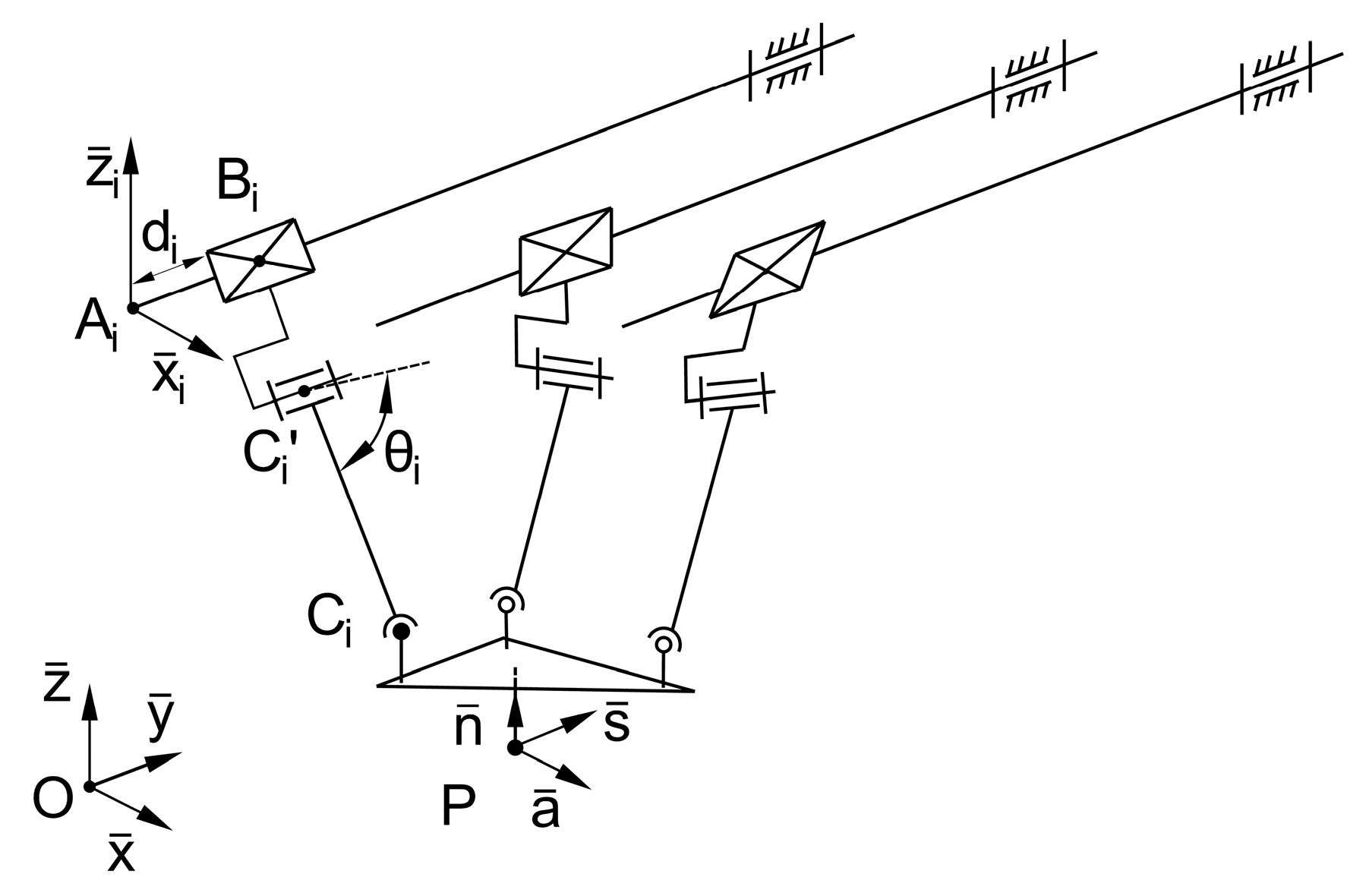
5.1. The 3RTRHU Robot Kinematics

Because the 3RTRHU robot has a symmetrical topology, the annotation is being shown for only one kinematic chain, to prevent Figure 6 from becoming overly cluttered. The notation contains the index i, offering the possibility to refer to the ith kinematic chain by i ∈ {1, 2, 3}. The moving platform of the robot, defined by the equilateral triangle C_1 C_2 C_3, contains the characteristic point P, which has the Pasn coordinate system attached to it. The length of the sides of the triangle is denoted by c, and the distance of the point P from the platform is denoted by l. The projection of point P is the centroid of the triangle.

The moving platform is linked to the base by the three kinematic chains, as presented in Figure 6. Based on the d1 configuration in Figure 2, the kinematic chains consist of a rotational joint (with center $A_i$), a translational joint (with center $B_i$), a rotational joint (with center $C_i^{\prime }$), a helical joint (with center $C_i^{″}$ and pitch p), and a universal joint (with center $C_i$). The center points of the joints are defined by several parameters in

Table 3. Definition of joint center points to the $Oxyz$ coordinate system for the 3RTRHU kinematic chain.

Joint Center Points	Coordinates
	x	y	z
$A_1/A_2/A_3$	-s/0/s	0/0/0	0/0/0
$B_1/B_2/B_3$ and $B_i\equiv C_i^{\prime }\equiv C_i^{″}$	-s/0/s	$d_1$$/d_2$$/d_3$	0/0/0
$C_1$	$x_p-100\hspace{0.17em}\mathrm{c}{\beta }_P\hspace{0.17em}\mathrm{s}{\gamma }_p+{\displaystyle \frac{100\hspace{0.17em}\sqrt{3}\hspace{0.17em}\left(\mathrm{c}{\alpha }_p\hspace{0.17em}\mathrm{s}{\gamma }_p-\mathrm{c}{\gamma }_p\hspace{0.17em}\mathrm{s}{\alpha }_p\hspace{0.17em}\mathrm{s}{\beta }_p\right)}{3}}$	$y_p+100\hspace{0.17em}\mathrm{c}{\beta }_P\hspace{0.17em}\mathrm{s}{\gamma }_p-{\displaystyle \frac{100\hspace{0.17em}\sqrt{3}\hspace{0.17em}\left(\mathrm{c}{\alpha }_p\hspace{0.17em}\mathrm{c}{\gamma }_p-\mathrm{s}{\alpha }_p\hspace{0.17em}\mathrm{s}{\beta }_p\hspace{0.17em}\mathrm{s}{\gamma }_p\right)}{3}}$	$z_p+100\hspace{0.17em}\mathrm{s}{\beta }_p-{\displaystyle \frac{100\hspace{0.17em}\sqrt{3}\hspace{0.17em}\mathrm{c}{\beta }_p\mathrm{s}{\alpha }_p}{3}}$
$C_2$	$x_p-{\displaystyle \frac{200\hspace{0.17em}\sqrt{3}\hspace{0.17em}\left(\mathrm{c}{\alpha }_p\hspace{0.17em}\mathrm{s}{\gamma }_p-\mathrm{c}{\gamma }_p\hspace{0.17em}\mathrm{s}{\alpha }_p\hspace{0.17em}\mathrm{s}{\beta }_p\right)}{3}}$	$y_p+{\displaystyle \frac{200\hspace{0.17em}\sqrt{3}\left(\mathrm{c}{\alpha }_p\hspace{0.17em}\mathrm{c}{\gamma }_p-\mathrm{s}{\alpha }_p\hspace{0.17em}\mathrm{s}{\beta }_p\hspace{0.17em}\mathrm{s}{\gamma }_p\right)}{3}}$	$z_p+{\displaystyle \frac{200\hspace{0.17em}\sqrt{3}\hspace{0.17em}\mathrm{c}{\beta }_p\hspace{0.17em}\mathrm{s}{\alpha }_p}{3}}$
$C_3$	$x_p+100\hspace{0.17em}\mathrm{c}{\beta }_p\hspace{0.17em}\mathrm{c}{\gamma }_p+{\displaystyle \frac{100\hspace{0.17em}\sqrt{3}\hspace{0.17em}\left(\mathrm{c}{\alpha }_p\hspace{0.17em}\mathrm{s}{\gamma }_p-\mathrm{c}{\gamma }_p\hspace{0.17em}\mathrm{s}{\alpha }_p\hspace{0.17em}\mathrm{s}{\beta }_p\right)}{3}}$	$y_p-100\hspace{0.17em}\mathrm{c}\beta \hspace{0.17em}\mathrm{s}{\gamma }_p-{\displaystyle \frac{100\hspace{0.17em}\sqrt{3}\hspace{0.17em}\left(\mathrm{c}{\alpha }_p\hspace{0.17em}\mathrm{c}{\gamma }_p-\mathrm{s}{\alpha }_p\hspace{0.17em}\mathrm{s}{\beta }_p\hspace{0.17em}\mathrm{s}{\gamma }_p\right)}{3}}$	$z_p-100\hspace{0.17em}\hspace{0.17em}\mathrm{s}{\beta }_p-{\displaystyle \frac{100\hspace{0.17em}\sqrt{3}\hspace{0.17em}\mathrm{c}{\beta }_p\mathrm{s}{\alpha }_p}{3}}$

Observation: As seen in the first row, $A_2{x}_2{y}_2{z}_2\equiv Oxyz$. The origin of the coordinate systems $A_1{x}_1{y}_1{z}_1$ ad $A_3{x}_3{y}_3{z}_3$ are lying on the Ox axis, having the coordinates ${|x}_{A1}|=x_{A3}=s$, and the axes are parallel with the axes of $Oxyz$.

. It is regarded that $B_i\equiv C_i^{\prime }\equiv C_i^{″}$, and, thus, a simplified mathematical model is acquired. A robot can be designed based on the simplified model [64], but this is beyond the scope of this study.

The definition of the $C_i$ center points is given by using the ${}^0\mathit{X}$ generalized coordinates vector (by use of a homogeneous transformation matrix concerning the Oxyz system) and the constant relative position ${}^P{C}_i$ with respect to the $Pasn$ coordinate system, as follows:

$$\left[\begin{array}{c}{C}_i\\ 1\end{array}\right]=T\left(x_P,y_P,z_P,{\alpha }_P,{\beta }_P,{\gamma }_P\right)\left[\begin{array}{c}{}^P{C}_i\\ 1\end{array}\right]$$

(39)

Another essential mathematical relation for the geometric model of the mechanism is the length of the link $B_i{C}_i$ denoted by $h_i$:

$$h_i={\displaystyle \frac{p}{2\pi }}{\theta }_i,$$

(40)

where p [mm] is the pitch of the helical joint, and ${\theta }_i$ [rad] is the rotation angle induced by the joint $C_i\mathrm{”}$.

Defining the $C_i$ center points through the $O-A_i-B_i-C_i”-C_i\prime$ kinematic chains (using the parameters from Table 3, as well Equation (40)), the following loop closure equations are acquired:

$$\begin{array}{l}{f}_1:d_1-y_P-100\hspace{0.17em}\mathrm{c}{\beta }_P\hspace{0.17em}\mathrm{s}{\gamma }_P+{\displaystyle \frac{100\hspace{0.17em}\sqrt{3}\hspace{0.17em}\left(\mathrm{c}{\alpha }_P\hspace{0.17em}\mathrm{c}{\gamma }_P-\mathrm{s}{\alpha }_P\hspace{0.17em}\mathrm{s}{\beta }_P\hspace{0.17em}\mathrm{s}{\gamma }_P\right)}{3}}=0;\\ f_2:{\displaystyle \frac{p^2}{4{\pi }^2}}{\theta }_1^2-{\left(z_P+100\hspace{0.17em}\mathrm{s}{\beta }_p-{\displaystyle \frac{100\hspace{0.17em}\sqrt{3}\hspace{0.17em}\mathrm{c}{\beta }_P\hspace{0.17em}\mathrm{s}{\alpha }_P}{3}}\right)}^2-{\left(x_{\mathrm{B}1}-x_P+100\hspace{0.17em}\mathrm{c}{\beta }_P\mathrm{c}{\gamma }_P-{\displaystyle \frac{100\hspace{0.17em}\sqrt{3}\hspace{0.17em}\left(\mathrm{c}{\alpha }_P\mathrm{s}{\gamma }_P-\mathrm{c}{\gamma }_P\hspace{0.17em}\mathrm{s}{\alpha }_P\hspace{0.17em}\mathrm{s}{\beta }_P\right)}{3}}\right)}^2=0;\\ f_3:d_2-y_P-{\displaystyle \frac{200\hspace{0.17em}\sqrt{3}\hspace{0.17em}\left(\mathrm{c}{\alpha }_P\hspace{0.17em}\mathrm{c}{\gamma }_P-\mathrm{s}{\alpha }_P\hspace{0.17em}\mathrm{s}{\beta }_P\hspace{0.17em}\mathrm{s}{\gamma }_P\right)}{3}}=0;\\ f_4:{\displaystyle \frac{p^2}{4{\pi }^2}}{\theta }_2^2-{\left(z_P+{\displaystyle \frac{200\hspace{0.17em}\sqrt{3}\hspace{0.17em}\mathrm{c}{\beta }_P\hspace{0.17em}\mathrm{s}{\alpha }_P}{3}}\right)}^2-{\left(x_P-{\displaystyle \frac{200\hspace{0.17em}\sqrt{3}\hspace{0.17em}\left(\mathrm{c}{\alpha }_P\hspace{0.17em}\mathrm{s}{\gamma }_P-\mathrm{c}{\gamma }_P\hspace{0.17em}\mathrm{s}{\alpha }_P\hspace{0.17em}\mathrm{s}{\beta }_P\right)}{3}}\right)}^2=0;\\ f_5:d_3-y_P+100\hspace{0.17em}\mathrm{c}{\beta }_P\hspace{0.17em}\mathrm{s}{\gamma }_P+{\displaystyle \frac{100\hspace{0.17em}\sqrt{3}\hspace{0.17em}\left(\mathrm{c}{\alpha }_P\hspace{0.17em}\mathrm{c}{\gamma }_P-\mathrm{s}{\alpha }_P\hspace{0.17em}\mathrm{s}{\beta }_P\hspace{0.17em}\mathrm{s}{\gamma }_P\right)}{3}}=0;\\ f_6:{\displaystyle \frac{p^2}{4{\pi }^2}}{\theta }_3^2-{\left(100\hspace{0.17em}\mathrm{s}{\beta }_P-z_P+{\displaystyle \frac{100\hspace{0.17em}\sqrt{3}\hspace{0.17em}\mathrm{c}{\beta }_P\hspace{0.17em}\mathrm{s}{\alpha }_P}{3}}\right)}^2-{\left(x_P-x_{\mathrm{B}3}+100\hspace{0.17em}\mathrm{c}{\beta }_P\hspace{0.17em}\mathrm{c}{\gamma }_P+{\displaystyle \frac{100\hspace{0.17em}\sqrt{3}\hspace{0.17em}\left(\mathrm{c}{\alpha }_P\hspace{0.17em}\mathrm{s}{\gamma }_P-\mathrm{c}{\gamma }_P\hspace{0.17em}\mathrm{s}{\alpha }_P\hspace{0.17em}\mathrm{s}{\beta }_P\right)}{3}}\right)}^2=0\end{array}$$

(41)

In order to be able to draw some conclusions about this robot mechanism, A and B matrices (Equation (35)) are simplified by substituting numerical values into the equation. The distance is set to $l=0\mathrm{m}\mathrm{m}$, the platform side length is set to $c=200\mathrm{m}\mathrm{m}$, and the pitch of the helical joint is set to $p=10\mathrm{m}\mathrm{m}$. Moreover, using the Euler angles set to zero (${\alpha }_P={\beta }_P={\gamma }_P=0$), no rotation of the platform with respect to the Oxyz coordinate system has to be considered:

$$A=\left(\begin{array}{cccccc}0& -1& 0& 0& 0& -100\\ 2\hspace{0.17em}(x_{B1}-\hspace{0.17em}{x}_p+100)& 0& -2\hspace{0.17em}{z}_p& {\displaystyle \frac{200\sqrt{3}}{3}}{z}_p& -200\hspace{0.17em}{z}_p& {\displaystyle \frac{200\hspace{0.17em}\sqrt{3}\hspace{0.17em}}{3}}\left(x_{B1}-x_p+100\right)\\ 0& -1& 0& 0& 0& 0\\ -2\hspace{0.17em}{x}_p& 0& -2\hspace{0.17em}{z}_p& -{\displaystyle \frac{400\sqrt{3}}{3}}{z}_p& 0& {\displaystyle \frac{400\sqrt{3}}{3}}{x}_p\\ 0& -1& 0& 0& 0& 100\\ 2(\hspace{0.17em}{x}_{B3}-\hspace{0.17em}{x}_p-100)& 0& -2\hspace{0.17em}{z}_p& {\displaystyle \frac{200\sqrt{3}}{3}}{z}_p& 200\hspace{0.17em}{z}_p& {\displaystyle \frac{200\hspace{0.17em}\sqrt{3}\hspace{0.17em}}{3}}\left(x_{B3}-x_p-100\right)\end{array}\right),$$

(42)

$$B=\left(\begin{array}{cccccc}1& 0& 0& 0& 0& 0\\ 0& {\displaystyle \frac{20}{{\pi }^2}}{\theta }_1& 0& 0& 0& 0\\ 0& 0& 1& 0& 0& 0\\ 0& 0& 0& {\displaystyle \frac{20}{{\pi }^2}}{\theta }_2& 0& 0\\ 0& 0& 0& 0& 1& 0\\ 0& 0& 0& 0& 0& {\displaystyle \frac{20}{{\pi }^2}}{\theta }_3\end{array}\right).$$

(43)

To search for singular configurations, the determinants of the matrices from Equations (42) and (43) are examined. As the first case, an obvious condition for $det\left(A\right)=0$ is when $z_P$ equals zero (resulting in zero columns for the third, fourth and fifth columns). This means that the characteristic point P will lie in the xOy plane. However, as observed in Figure 6, this plane contains the axes of the $A_i$ and $B_i$ joints, so it is impossible to physically implement this configuration. A second case for a zero determinant is identified by having zero values for the first and sixth columns:

$$\left\{\begin{array}{c}{x}_{B1}-\hspace{0.17em}{x}_p+100=0\\ x_p=0\\ x_{B3}-\hspace{0.17em}{x}_p-100=0\end{array}\right.$$

(44)

The straightforward solutions for the above system of equations are $x_p=0$, $x_{B1}=-100$ and $x_{B3}=100$. These values result in a mechanism configuration where the kinematic chains linking the mobile platform to the base are parallel to one another ($B_1{C}_1\parallel B_2{C}_2\parallel B_3{C}_3$). In this singular configuration, the mechanism acquires an uncontrolled degree of freedom. Even if a specific set of numerical values is applied to some parameters, the singular configuration would arise as long as the condition of $\left|x_{B1}\right|=x_{B3}=p/2$ is met. This condition can be easily avoided by a careful geometrical dimensioning of the robot mechanism by making sure that the distances between the axes of the rotational joints $A_1$ and $A_2$, as well as the axes of $A_2$ and $A_3$, differ from the half-length of the side of the platform.

The mechanism also yields singular configurations for the ${\theta }_i=0\left(i=1,2,3\right)$ parameter values, those leading to $det\left(B\right)=0$. Based on Equation (40), the above ${\theta }_i$ values lead to $h_i=0$ condition, which means that the $B_i$ and $C_i$ joints superimpose. In the case of a physical model, this is unfeasible, so such a singularity should be circumvented.

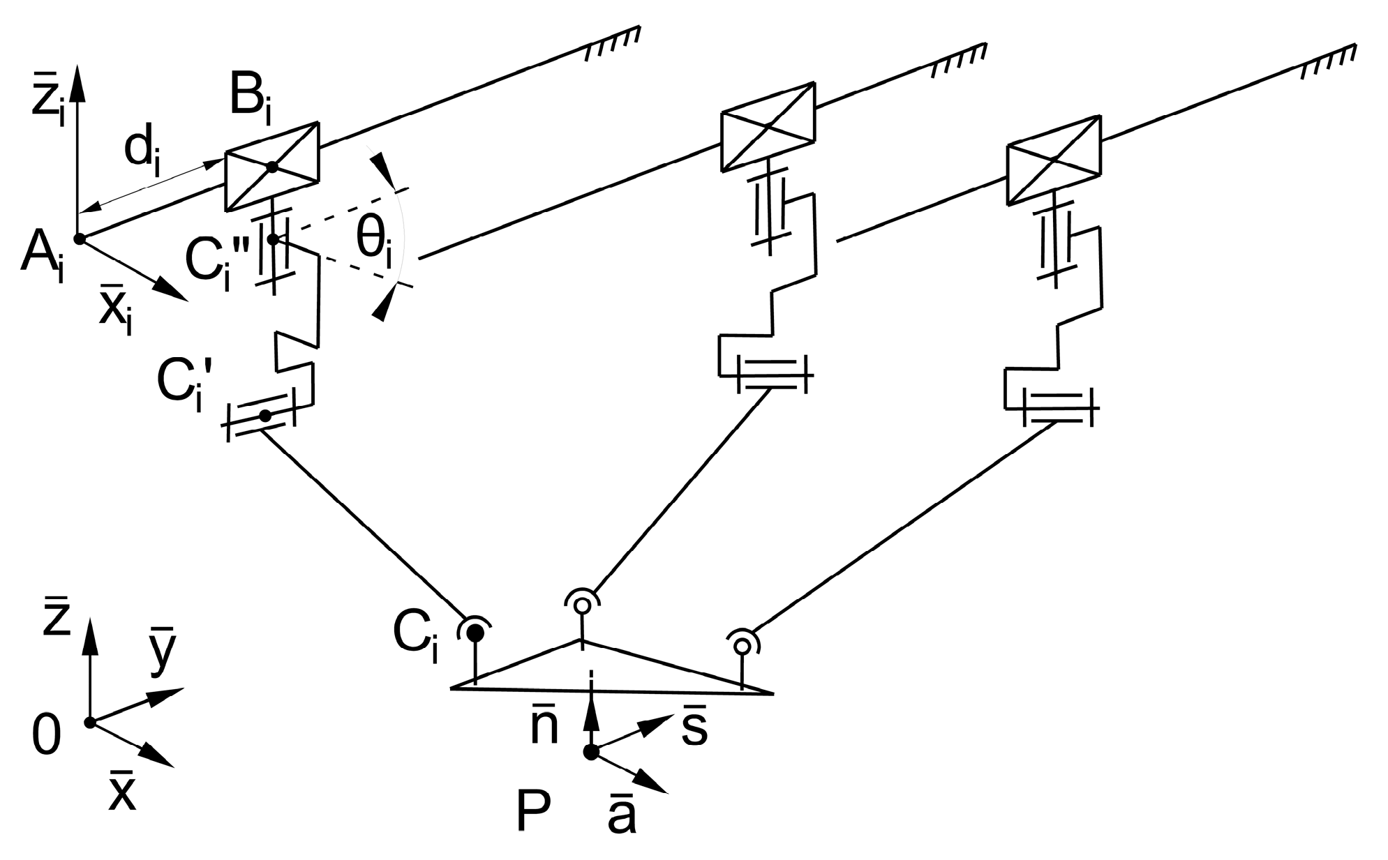
5.2. The 3RTRS Robot Kinematics

The RTRS kinematic chain is slightly different from the RTRHU chain, since it consists of rotational, translational and rotational joints as the positioning mechanism (variant d₂ in Figure 2), completed by one spherical joint ($C_i$). It should be mentioned that the axes of joints $A_i$ and $B_i$ are coincident, and the axes of joints $B_i$ and $C_i^{\prime }$ are perpendicular (Figure 7).

The position of $C_i$ in the $Oxyz$ coordinate system is determined by Equation (39) and Table 3, and the other joint centers are defined according to

Table 4. Definition of joint center points defined in the $Oxyz$ coordinate system for the 3RTRS.

Joint Center Points	Coordinates
	x	y	z
$A_1/A_2/A_3$	-s/0/s	0/0/0	0/0/0
$B_1/B_2/B_3$ and $B_i\equiv C_i^{\prime }$	-s/0/s	$d_1$$/d_2$$/d_3$	0/0/0

. It can be seen that the distance of $B_i{C}_i^{\prime }$ is maintained at zero, in order to have a simpler mathematical model, and a physical model can also be developed with this distance value.

By defining the length of the $C_i\prime C_i$ link as $h\left[\mathrm{mm}\right]$, as well as the sine and cosine of the ${\theta }_i$ angle as $s{\theta }_i$ and $c{\theta }_i$, the loop closure equations can be written as follows:

$$\begin{array}{l}{f}_1:d_1-y_p+h\hspace{0.17em}\mathrm{c}{\theta }_1-100\hspace{0.17em}\mathrm{c}{\beta }_p\hspace{0.17em}\mathrm{s}{\gamma }_p+{\displaystyle \frac{100\hspace{0.17em}\sqrt{3}\hspace{0.17em}\left(\mathrm{c}{\alpha }_p\hspace{0.17em}\mathrm{c}{\gamma }_p-\mathrm{s}{\alpha }_p\hspace{0.17em}\mathrm{s}{\beta }_p\hspace{0.17em}\mathrm{s}{\gamma }_p\right)}{3}}=0;\\ f_2:h^2\hspace{0.17em}{\mathrm{s}}^2{\theta }_1-{\left(z_p+100\hspace{0.17em}\mathrm{s}{\beta }_p-{\displaystyle \frac{100\hspace{0.17em}\sqrt{3}\hspace{0.17em}\mathrm{c}{\beta }_p\hspace{0.17em}\mathrm{s}{\alpha }_p}{3}}\right)}^2-{\left(x_{\mathrm{B}1}-x_p+100\hspace{0.17em}\mathrm{c}{\beta }_{p}c{\gamma }_p-{\displaystyle \frac{100\hspace{0.17em}\sqrt{3}\hspace{0.17em}\left(\mathrm{c}{\alpha }_p\hspace{0.17em}\mathrm{s}{\gamma }_p-\mathrm{c}{\gamma }_p\hspace{0.17em}\mathrm{s}{\alpha }_p\hspace{0.17em}\mathrm{s}{\beta }_p\right)}{3}}\right)}^2=0;\\ f_3:d_2-y_p+h\hspace{0.17em}\mathrm{c}{\theta }_2-{\displaystyle \frac{200\hspace{0.17em}\sqrt{3}\hspace{0.17em}\left(\mathrm{c}{\alpha }_p\hspace{0.17em}\mathrm{c}{\gamma }_p-\mathrm{s}{\alpha }_p\hspace{0.17em}\mathrm{s}{\beta }_p\hspace{0.17em}\mathrm{s}{\gamma }_p\right)}{3}}=0;\\ f_4:h^2\hspace{0.17em}{\mathrm{s}}^2{\theta }_2-{\left(x_p-{\displaystyle \frac{200\hspace{0.17em}\sqrt{3}\hspace{0.17em}\left(\mathrm{c}{\alpha }_p\hspace{0.17em}\mathrm{s}{\gamma }_p-\mathrm{c}{\gamma }_p\hspace{0.17em}\mathrm{s}{\alpha }_p\hspace{0.17em}\mathrm{s}{\beta }_p\right)}{3}}\right)}^2-{\left(z_p+{\displaystyle \frac{200\hspace{0.17em}\sqrt{3}\hspace{0.17em}\mathrm{c}{\beta }_p\hspace{0.17em}\mathrm{s}{\alpha }_p}{3}}\right)}^2=0;\\ f_5:d_3-y_p+h\hspace{0.17em}\mathrm{c}{\theta }_3+100\hspace{0.17em}\mathrm{c}{\beta }_p\hspace{0.17em}\mathrm{s}{\gamma }_p+{\displaystyle \frac{100\hspace{0.17em}\sqrt{3}\hspace{0.17em}\left(\mathrm{c}{\alpha }_p\hspace{0.17em}\mathrm{c}{\gamma }_p-\mathrm{s}{\alpha }_p\hspace{0.17em}\mathrm{s}{\beta }_p\hspace{0.17em}\mathrm{s}{\gamma }_p\right)}{3}}=0;\\ f_6:h^2\hspace{0.17em}{\mathrm{s}}^2{\theta }_3-{\left(100\hspace{0.17em}\mathrm{s}{\beta }_p-z_p+{\displaystyle \frac{100\hspace{0.17em}\sqrt{3}\hspace{0.17em}\mathrm{c}{\beta }_p\hspace{0.17em}\mathrm{s}{\alpha }_p}{3}}\right)}^2-{\left(x_p-x_{\mathrm{B}3}+100\hspace{0.17em}\mathrm{c}{\beta }_p\hspace{0.17em}\mathrm{c}{\gamma }_p+{\displaystyle \frac{100\hspace{0.17em}\sqrt{3}\hspace{0.17em}\left(\mathrm{c}{\alpha }_p\hspace{0.17em}\mathrm{s}{\gamma }_p-\mathrm{c}{\gamma }_p\hspace{0.17em}\mathrm{s}{\alpha }_p\hspace{0.17em}\mathrm{s}{\beta }_p\right)}{3}}\right)}^2=0.\end{array}$$

(45)

In the case of the 3RTRS robot, the matrices A and B from kinematic Equation (35) are redefined. As in the previous case, the same numerical values are applied in order to be able to acquire a simplified form for the matrices and to establish some singular configuration conditions. In addition, $l=0\mathrm{m}\mathrm{m}$ and $c=200\mathrm{m}\mathrm{m}$; the length of the $C_i\prime C_i$ link is set to $h=400\mathrm{m}\mathrm{m}$.

$$A=\left(\begin{array}{cccccc}0& -1& 0& 0& 0& -100\\ 2\hspace{0.17em}(x_{B1}-\hspace{0.17em}{x}_p+100)& 0& -2\hspace{0.17em}{z}_p& {\displaystyle \frac{200\sqrt{3}}{3}}{z}_p& -200\hspace{0.17em}{z}_p& {\displaystyle \frac{200\hspace{0.17em}\sqrt{3}\hspace{0.17em}}{3}}\left(x_{B1}-x_p+100\right)\\ 0& -1& 0& 0& 0& 0\\ -2\hspace{0.17em}{x}_p& 0& -2\hspace{0.17em}{z}_p& -{\displaystyle \frac{400\sqrt{3}}{3}}{z}_p& 0& {\displaystyle \frac{400\sqrt{3}}{3}}{x}_p\\ 0& -1& 0& 0& 0& 100\\ 2(\hspace{0.17em}{x}_{B3}-\hspace{0.17em}{x}_p-100)& 0& -2\hspace{0.17em}{z}_p& {\displaystyle \frac{200\sqrt{3}}{3}}{z}_p& 200\hspace{0.17em}{z}_p& {\displaystyle \frac{200\hspace{0.17em}\sqrt{3}\hspace{0.17em}}{3}}\left(x_{B3}-x_p-100\right)\end{array}\right)$$

(46)

$$B=\left(\begin{array}{cccccc}1& -400\hspace{0.17em}\mathrm{s}{\theta }_1& 0& 0& 0& 0\\ 0& 320000\hspace{0.17em}\mathrm{c}{\theta }_1\hspace{0.17em}\mathrm{s}{\theta }_1& 0& 0& 0& 0\\ 0& 0& 1& -400\hspace{0.17em}\mathrm{s}{\theta }_2& 0& 0\\ 0& 0& 0& 320000\hspace{0.17em}\mathrm{c}{\theta }_2\hspace{0.17em}\mathrm{s}{\theta }_2& 0& 0\\ 0& 0& 0& 0& 1& -400\hspace{0.17em}\mathrm{s}{\theta }_3\\ 0& 0& 0& 0& 0& 320000\hspace{0.17em}\mathrm{c}{\theta }_3\hspace{0.17em}\mathrm{s}{\theta }_3\end{array}\right)$$

(47)

It is straightforward that Equations (42) and (46) are identical, so the conditions to have $det\left(A\right)=0$ are the same as in the previous sub-section. The same equalities (44) hold true here as well, leading to the same singular configuration.

The matrix B is slightly different from its form in Equation (43), leading to other singular configurations characteristic of the 3RTRS robot. The $det\left(B\right)=0$ is true in the case of any ${\theta }_i=0$ or ${\theta }_i=\pi /2$. If we set the distance $B_i{C}_i^{\prime }=0$, as it is supposed to be in the loop closure equations, ${\theta }_i=0$ means that the $C_i^{\prime }{C}_i$ link is folded onto the $B_i$ axis, having an infinite number of solutions for the $A_i$ rotational joint value in the case of inverse modeling. This overlapping configuration is easily avoided in the physical mechanism due to its real geometrical dimensions (width and height of the physical components). The ${\theta }_i=\pi /2$ means that the $C_i^{\prime }{C}_i$ link is perpendicular to the $B_i$ axis, so the $C_1{C}_2{C}_3$ platform is not able to move with its $C_i$ joint in the direction of the $C_i^{\prime }{C}_i$ link, not even towards the inner part of the workspace. Those singular configurations should be avoided by the control algorithm.

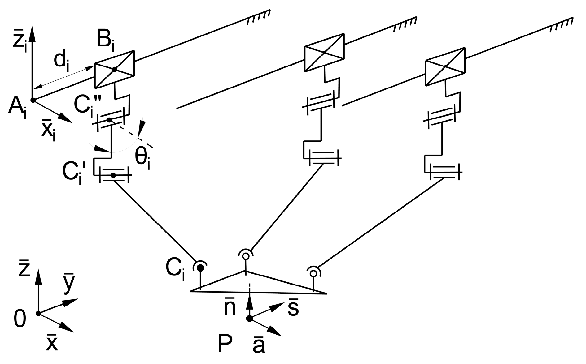
5.3. The 3TRRS^I Robot Kinematics

If the linkage variant (e1) from Figure 2 is completed with a spherical joint ($C_i$), the kinematic chain TRRS is built as part of the 6-DoF mechanism named 3TRRSI. The index I is used to indicate that it is the first variant with this series of joint types to be examined. It must be noted that the variant (e1) has perpendicular axes for the first two, a translational ($B_i$) and a rotational ($C_i^{″}$) joint. This feature renders the mechanism an excellent option for the application of the double-actuation module presented in Figure 1, where the same perpendicularity is present between the two translational and rotational output axes.

The axes of the joints $C_i^{″}$ and $C_i^{\prime }$ are perpendicular as well (Figure 8). For mathematical simplicity, the identity of the $B_i\equiv C_i^{″}\equiv C_i^{\prime }$ is applicable (without losing generality) by applying the notations for the joint coordinates from Table 3, as well the same h [mm] notation for the link length $C_i^{\prime }{C}_i$ as in previous sub-section.

Using the above annotations and considerations, the six geometrical loop closure equations can be written for the 3TRRS^I robot mechanism as follows:

$$\begin{array}{l}{f}_1:-\sqrt{{\left(x_{\mathrm{B}1}-x_p+100\hspace{0.17em}\mathrm{c}{\beta }_p\hspace{0.17em}\mathrm{c}{\gamma }_p-{\displaystyle \frac{100\hspace{0.17em}\sqrt{3}\hspace{0.17em}\left(\mathrm{c}{\alpha }_p\hspace{0.17em}\mathrm{s}{\gamma }_p-\mathrm{c}{\gamma }_p\hspace{0.17em}\mathrm{s}{\alpha }_p\hspace{0.17em}\mathrm{s}{\beta }_p\right)}{3}}\right)}^2}-\\ \hspace{1em}\hspace{1em}\hspace{1em}\hspace{1em}\hspace{1em}\hspace{1em}-\mathrm{t}\mathrm{g}{\theta }_1\hspace{0.17em}\left(d_1-y_p-100\hspace{0.17em}\mathrm{c}{\beta }_p\hspace{0.17em}\mathrm{s}{\gamma }_p+{\displaystyle \frac{100\hspace{0.17em}\sqrt{3}\hspace{0.17em}\left(\mathrm{c}{\alpha }_p\hspace{0.17em}\mathrm{c}{\gamma }_p-\mathrm{s}{\alpha }_p\hspace{0.17em}\mathrm{s}{\beta }_p\hspace{0.17em}\mathrm{s}{\gamma }_p\right)}{3}}\right)=0;\\ f_2:h^2-{\left(d_1-y_p-100\hspace{0.17em}\mathrm{c}{\beta }_{p}s{\gamma }_p+{\displaystyle \frac{100\hspace{0.17em}\sqrt{3}\hspace{0.17em}\left(\mathrm{c}{\alpha }_p\hspace{0.17em}\mathrm{c}{\gamma }_p-\mathrm{s}{\alpha }_p\hspace{0.17em}\mathrm{s}{\beta }_p\hspace{0.17em}\mathrm{s}{\gamma }_p\right)}{3}}\right)}^2-\\ \hspace{1em}\hspace{1em}\hspace{1em}\hspace{1em}\hspace{1em}\hspace{1em}-{\left(x_{\mathrm{B}1}-x_p+100\hspace{0.17em}\mathrm{c}{\beta }_p\hspace{0.17em}\mathrm{c}{\gamma }_p-{\displaystyle \frac{100\hspace{0.17em}\sqrt{3}\hspace{0.17em}\left(\mathrm{c}{\alpha }_p\hspace{0.17em}\mathrm{s}{\gamma }_p-\mathrm{c}{\gamma }_p\hspace{0.17em}\mathrm{s}{\alpha }_p\hspace{0.17em}\mathrm{s}{\beta }_p\right)}{3}}\right)}^2-{\left(z_p+100\hspace{0.17em}\mathrm{s}{\beta }_p-{\displaystyle \frac{100\hspace{0.17em}\sqrt{3}\hspace{0.17em}\mathrm{c}{\beta }_p\hspace{0.17em}\mathrm{s}{\alpha }_p}{3}}\right)}^2=0;\\ f_3:\mathrm{t}\mathrm{g}{\theta }_2\hspace{0.17em}\left(y_p-d_2+{\displaystyle \frac{200\hspace{0.17em}\sqrt{3}\hspace{0.17em}\left(\mathrm{c}{\alpha }_p\hspace{0.17em}\mathrm{c}{\gamma }_p-\mathrm{s}{\alpha }_p\hspace{0.17em}\mathrm{s}{\beta }_p\hspace{0.17em}\mathrm{s}{\gamma }_p\right)}{3}}\right)-\sqrt{{\left(x_{\mathrm{B}2}-x_p+{\displaystyle \frac{200\hspace{0.17em}\sqrt{3}\hspace{0.17em}\left(\mathrm{c}{\alpha }_p\hspace{0.17em}\mathrm{s}{\gamma }_p-\mathrm{c}{\gamma }_p\hspace{0.17em}\mathrm{s}{\alpha }_p\hspace{0.17em}\mathrm{s}{\beta }_p\right)}{3}}\right)}^2}=0;\\ f_4:h^2-{\left(z_p+{\displaystyle \frac{200\hspace{0.17em}\sqrt{3}\hspace{0.17em}\mathrm{c}{\beta }_p\hspace{0.17em}\mathrm{s}{\alpha }_p}{3}}\right)}^2-{\left(y_p-d_2+{\displaystyle \frac{200\hspace{0.17em}\sqrt{3}\hspace{0.17em}\left(\mathrm{c}{\alpha }_p\hspace{0.17em}\mathrm{c}{\gamma }_p-\mathrm{s}{\alpha }_p\hspace{0.17em}\mathrm{s}{\beta }_p\hspace{0.17em}\mathrm{s}{\gamma }_p\right)}{3}}\right)}^2-{\left(x_{\mathrm{B}2}-x_p+{\displaystyle \frac{200\hspace{0.17em}\sqrt{3}\hspace{0.17em}\left(\mathrm{c}{\alpha }_p\hspace{0.17em}\mathrm{s}{\gamma }_p-\mathrm{c}{\gamma }_{p}s{\alpha }_p\hspace{0.17em}\mathrm{s}{\beta }_p\right)}{3}}\right)}^2=0;\\ f_5:-\sqrt{{\left(x_p-x_{\mathrm{B}3}+100\hspace{0.17em}\mathrm{c}{\beta }_p\hspace{0.17em}\mathrm{c}{\gamma }_p+{\displaystyle \frac{100\hspace{0.17em}\sqrt{3}\hspace{0.17em}\left(\mathrm{c}{\alpha }_p\hspace{0.17em}\mathrm{s}{\gamma }_p-\mathrm{c}{\gamma }_p\hspace{0.17em}\mathrm{s}{\alpha }_p\hspace{0.17em}\mathrm{s}{\beta }_p\right)}{3}}\right)}^2}-\\ \hspace{1em}\hspace{1em}\hspace{1em}\hspace{1em}\hspace{1em}\hspace{1em}-\mathrm{t}\mathrm{g}{\theta }_3\hspace{0.17em}\left(d_3-y_p+100\hspace{0.17em}\mathrm{c}{\beta }_p\mathrm{s}{\gamma }_p+{\displaystyle \frac{100\hspace{0.17em}\sqrt{3}\hspace{0.17em}\left(\mathrm{c}{\alpha }_p\hspace{0.17em}\mathrm{c}{\gamma }_p-\mathrm{s}{\alpha }_p\hspace{0.17em}\mathrm{s}{\beta }_p\hspace{0.17em}\mathrm{s}{\gamma }_p\right)}{3}}\right)=0;\\ f_6:h^2-{\left(d_3-y_p+100\hspace{0.17em}\mathrm{c}{\beta }_p\hspace{0.17em}\mathrm{s}{\gamma }_p+{\displaystyle \frac{100\hspace{0.17em}\sqrt{3}\hspace{0.17em}\left(\mathrm{c}{\alpha }_p\hspace{0.17em}\mathrm{c}{\gamma }_p-\mathrm{s}{\alpha }_p\hspace{0.17em}\mathrm{s}{\beta }_p\hspace{0.17em}\mathrm{s}{\gamma }_p\right)}{3}}\right)}^2-\\ \hspace{1em}\hspace{1em}\hspace{1em}\hspace{1em}\hspace{1em}\hspace{1em}-{\left(x_p-x_{\mathrm{B}3}+100\hspace{0.17em}\mathrm{c}{\beta }_p\hspace{0.17em}\mathrm{c}{\gamma }_p+{\displaystyle \frac{100\hspace{0.17em}\sqrt{3}\hspace{0.17em}\left(\mathrm{c}{\alpha }_{p}s{\gamma }_p-\mathrm{c}{\gamma }_p\mathrm{s}{\alpha }_p\hspace{0.17em}\mathrm{s}{\beta }_p\right)}{3}}\right)}^2-{\left(100\hspace{0.17em}\mathrm{s}{\beta }_p-z_p+{\displaystyle \frac{100\hspace{0.17em}\sqrt{3}\hspace{0.17em}\mathrm{c}{\beta }_p\hspace{0.17em}\mathrm{s}{\alpha }_p}{3}}\right)}^2=0.\end{array}$$

(48)

As in the previous cases, numerical values are applied to be able to present a simplified form of the matrices A and B and to establish some singular configuration conditions: in addition to the $l=0\mathrm{m}\mathrm{m}$ and $c=200\mathrm{m}\mathrm{m}$ platform parameters, the length of the $C_i\prime C_i$ link is kept at $h=400\mathrm{m}\mathrm{m}$, and $x_{B2}=0\mathrm{m}\mathrm{m}$ means that the $Oxyz$ and $A_2{x}_2{y}_2{c}_2$ coordinate systems are coincident. Applying these values, the components of the Jacobian matrices are found, as follows:

$$A=\left(\begin{array}{cccccc}1& \mathrm{t}\mathrm{g}{\theta }_1& 0& 0& 0& 100\left(\hspace{0.17em}\mathrm{t}\mathrm{g}{\theta }_1+{\displaystyle \frac{1\hspace{0.17em}\hspace{0.17em}}{\sqrt{3}\hspace{0.17em}}}\right)\\ 2\hspace{0.17em}\left(x_{\mathrm{B}1}-\hspace{0.17em}{x}_p+100\right)& 2\hspace{0.17em}{Y}_1& -2\hspace{0.17em}{z}_p& {\displaystyle \frac{200\hspace{0.17em}}{\sqrt{3}}}{z}_p& -200\hspace{0.17em}{z}_p& 200\hspace{0.17em}\left(Y_1+{\displaystyle \frac{x_{\mathrm{B}1}-x_p+100}{\sqrt{3}}}\right)\\ 1& \mathrm{t}\mathrm{g}{\theta }_2& 0& 0& 0& -{\displaystyle \frac{200\hspace{0.17em}\hspace{0.17em}}{\sqrt{3}\hspace{0.17em}}}\\ -2x_p\hspace{0.17em}& -2Y_2& -2\hspace{0.17em}{z}_p& -{\displaystyle \frac{400}{\sqrt{3}}}{z}_p& 0& {\displaystyle \frac{400}{\sqrt{3}}}{x}_p\\ 1& \mathrm{t}\mathrm{g}{\theta }_3& 0& 0& 0& -100\hspace{0.17em}\left(\mathrm{t}\mathrm{g}{\theta }_3-{\displaystyle \frac{1\hspace{0.17em}\hspace{0.17em}}{\sqrt{3}\hspace{0.17em}}}\right)\\ 2\hspace{0.17em}\left(x_{\mathrm{B}3}-x_p-100\right)& 2Y_3& -2\hspace{0.17em}{z}_p& {\displaystyle \frac{200\hspace{0.17em}}{\sqrt{3}}}{z}_p& 200\hspace{0.17em}{z}_p& 200\hspace{0.17em}\left(Y_3-{\displaystyle \frac{x_{\mathrm{B}3}-x_p-100}{\sqrt{3}}}\right)\end{array}\right)$$

(49)

$$B=\left(\begin{array}{cccccc}-\mathrm{t}\mathrm{g}{\theta }_1& -T_1\hspace{0.17em}{Y}_1& 0& 0& 0& 0\\ -2Y_1& 0& 0& 0& 0& 0\\ 0& 0& -\mathrm{t}\mathrm{g}{\theta }_2& T_2\hspace{0.17em}{Y}_2& 0& 0\\ 0& 0& 2Y_2& 0& 0& 0\\ 0& 0& 0& 0& -\mathrm{t}\mathrm{g}{\theta }_3& -T_3\hspace{0.17em}{Y}_3\\ 0& 0& 0& 0& -2Y_3& 0\end{array}\right),$$

(50)

where

$$\begin{gathered} \hspace{1em}{T}_1={\mathrm{t}\mathrm{g}}^2{\theta }_1+1,\hspace{1em}\hspace{1em}{T}_2={\mathrm{t}\mathrm{g}}^2{\theta }_2+1,\hspace{1em}\hspace{1em}{T}_3={\mathrm{t}\mathrm{g}}^2{\theta }_3+1 \\ {Y}_1=d_1-y_p+{\displaystyle \frac{100\hspace{0.17em}}{\sqrt{3}}},\hspace{1em}\hspace{1em}{Y_2=y}_p-d_2+{\displaystyle \frac{200\hspace{0.17em}}{\sqrt{3}}},\hspace{1em}\hspace{1em}{Y}_3=d_3-y_p+{\displaystyle \frac{100\hspace{0.17em}}{\sqrt{3}}} \end{gathered}$$

Even if the annotations $Y_i$ are used, it can be easily noticed that Equation (49) has similarities with the A matrices defined in the previous sub-sections.

To obtain $det\left(A\right)=0$, it is no longer sufficient to solely have the relations shown in (44) fulfilled, as the first column of the A matrix will not be entirely zero because of the constant 1 values. On the other hand, the zero determinant is realized when the expressions in the second column become zero ($tg{\theta }_i=0$ and $Y_i=0$ for $i=1,2,3$). This introduces the singular configuration in which ${\theta }_i=0$, meaning that the axes of joints $C_i^{\prime }$ are parallel with the Ox axis. The $Y_i=0$ condition is met when the $C_i\prime C_i$ links are parallel with the $xOz$ plane. Those two concomitant conditions lead to the setup where the $C_i\prime C_i$ links are parallel with the Oz axis, resulting in an uncontrolled degree of freedom for the mobile platform.

As with the previous mechanisms, the third, fourth and fifth columns will have zero values in the case of $z_p=0$, but, as stated earlier, because of the physical model dimensions, the characteristic point P cannot coincide with the plane defined by the $B_i$ axes. This kind of characteristic configuration can only occur in the mathematical model.

Another singular configuration will occur if ${\theta }_1={\theta }_3$. In this case, the first and the fifth row of the A matrix will be identical, so this leads to $det\left(A\right)=0$. Due to the aforementioned angular equality between the direction of axes of the $C_1^{\prime }$ and $C_3^{\prime }$ joints, and the spherical joints $C_i$ (which allows a rotation about the axes parallel with the axis of the $C_1^{\prime }$ joint), the $C_1^{\prime }{C}_1{C}_3{C}_3^{\prime }$ four-linkage mechanism gains an uncontrolled degree of freedom, having no active joint.

Examining Equation (50), the search for $det\left(B\right)=0$ conditions is more straightforward. It is obvious that the necessary and sufficient condition is as follows:

$$Y_1=0\mathrm{o}\mathrm{r}{Y}_2=0\mathrm{o}\mathrm{r}{Y}_3=0,$$

(51)

which means that any of the $C_i\prime C_i$ links are parallel with the $xOz$ plane and, hence, perpendicular to the axes of the $B_i$ joints (having in mind the assumption $B_i\equiv C_i″\equiv C_i\prime$ in Figure 8). This leads to a motion restriction for the $C_i$ joint center, hindering its displacement towards the inner part of the workspace in the direction of the $C_i\prime C_i$ link. In this case, the mechanism loses one degree of freedom.

5.4. The 3TRRS^II Robot Kinematics

The last examined parallel robot topology is presented in Figure 9, and based on the used symmetrical linkages, it is named 3TRRS^II. The mobile platform is linked to the base through the same type of joints as it was in the case of 3TRRS^I, but the positioning part of the linkages has one joint in a different orientation, following variant (c₁) in Figure 2. The linkages are completed by the usual $C_i$ spherical joints. The assumptions regarding the joint centers and the annotations used for geometrical dimensions are the same as in the case of the 3TRRS^I mechanism. The loop closure equations can be written in the following form:

$$\begin{array}{l}{f}_1:z_p+100\hspace{0.17em}\mathrm{s}{\beta }_p-\mathrm{t}\mathrm{g}{\theta }_1\hspace{0.17em}\sqrt{{\left(x_{\mathrm{B}1}-x_p+100\hspace{0.17em}\mathrm{c}{\beta }_p\hspace{0.17em}\mathrm{c}{\gamma }_p-{\displaystyle \frac{100}{\sqrt{3}}}\hspace{0.17em}\left(\mathrm{c}{\alpha }_p\hspace{0.17em}\mathrm{s}{\gamma }_p-\mathrm{c}{\gamma }_p\hspace{0.17em}\mathrm{s}{\alpha }_p\hspace{0.17em}\mathrm{s}{\beta }_p\right)\right)}^2}-{\displaystyle \frac{100}{\sqrt{3}}}\hspace{0.17em}\mathrm{c}{\beta }_p\hspace{0.17em}\mathrm{s}{\alpha }_p=0;\\ f_2:h^2-{\left(d_1-y_p-100\mathrm{c}{\beta }_p\hspace{0.17em}\mathrm{s}{\gamma }_p+{\displaystyle \frac{100}{\sqrt{3}\hspace{0.17em}}}\left(\mathrm{c}{\alpha }_p\hspace{0.17em}\mathrm{c}{\gamma }_p-\mathrm{s}{\alpha }_p\hspace{0.17em}\mathrm{s}{\beta }_p\hspace{0.17em}\mathrm{s}{\gamma }_p\right)\right)}^2-{\left(x_{\mathrm{B}1}-x_p+100\hspace{0.17em}\mathrm{c}{\beta }_p\hspace{0.17em}\mathrm{c}{\gamma }_p-{\displaystyle \frac{100}{\sqrt{3}}}\left(\mathrm{c}{\alpha }_p\hspace{0.17em}\mathrm{s}{\gamma }_p-\mathrm{c}{\gamma }_p\hspace{0.17em}\mathrm{s}{\alpha }_p\hspace{0.17em}\mathrm{s}{\beta }_p\right)\right)}^2-{\left(z_p+100\hspace{0.17em}\mathrm{s}{\beta }_p-{\displaystyle \frac{100}{3}}\mathrm{c}{\beta }_p\hspace{0.17em}\mathrm{s}{\alpha }_p\right)}^2=0;\\ f_3:z_p-\mathrm{t}\mathrm{g}{\theta }_2\hspace{0.17em}\sqrt{{\left(x_p-{\displaystyle \frac{200}{\sqrt{3}}}\left(\mathrm{c}{\alpha }_p\mathrm{s}{\gamma }_p-\mathrm{c}{\gamma }_p\hspace{0.17em}\mathrm{s}{\alpha }_p\hspace{0.17em}\mathrm{s}{\beta }_p\right)\right)}^2}+{\displaystyle \frac{200}{\sqrt{3}}}\mathrm{c}{\beta }_p\hspace{0.17em}\mathrm{s}{\alpha }_p=0;\\ f_4:h^2-{\left(z_p+{\displaystyle \frac{200}{\sqrt{3}}}\mathrm{c}{\beta }_p\hspace{0.17em}\mathrm{s}{\alpha }_p\right)}^2-{\left(y_p-d_2+{\displaystyle \frac{200}{\sqrt{3}}}\left(\mathrm{c}{\alpha }_p\hspace{0.17em}\mathrm{c}{\gamma }_p-\mathrm{s}{\alpha }_p\hspace{0.17em}\mathrm{s}{\beta }_p\hspace{0.17em}\mathrm{s}{\gamma }_p\right)\right)}^2-{\left(x_p-{\displaystyle \frac{200}{\sqrt{3}}}\left(\mathrm{c}{\alpha }_p\mathrm{s}{\gamma }_p-\mathrm{c}{\gamma }_p\hspace{0.17em}\mathrm{s}{\alpha }_p\hspace{0.17em}\mathrm{s}{\beta }_p\right)\right)}^2=0;\\ f_5:z_p-100\hspace{0.17em}\mathrm{s}{\beta }_p-\mathrm{t}\mathrm{g}{\theta }_3\hspace{0.17em}\sqrt{{\left(x_p-x_{\mathrm{B}3}+100\hspace{0.17em}\mathrm{c}{\beta }_p\hspace{0.17em}\mathrm{c}{\gamma }_p+{\displaystyle \frac{100}{\sqrt{3}\hspace{0.17em}}}\left(\mathrm{c}{\alpha }_p\hspace{0.17em}\mathrm{s}{\gamma }_p-\mathrm{c}{\gamma }_p\hspace{0.17em}\mathrm{s}{\alpha }_p\hspace{0.17em}\mathrm{s}{\beta }_p\right)\right)}^2}-{\displaystyle \frac{100}{\hspace{0.17em}\sqrt{3}}}\mathrm{c}{\beta }_p\hspace{0.17em}\mathrm{s}{\alpha }_p=0;\\ f_6:h^2-{\left(d_3-y_p+100\hspace{0.17em}\mathrm{c}{\beta }_p\hspace{0.17em}\mathrm{s}{\gamma }_p+{\displaystyle \frac{100}{\sqrt{3}}}\left(\mathrm{c}{\alpha }_p\hspace{0.17em}\mathrm{c}{\gamma }_p-\mathrm{s}{\alpha }_p\hspace{0.17em}\mathrm{s}{\beta }_p\hspace{0.17em}\mathrm{s}{\gamma }_p\right)\right)}^2-{\left(x_p-x_{\mathrm{B}3}+100\hspace{0.17em}\mathrm{c}{\beta }_p\hspace{0.17em}\mathrm{c}{\gamma }_p+{\displaystyle \frac{100}{\sqrt{3}}}\left(\mathrm{c}{\alpha }_p\hspace{0.17em}\mathrm{s}{\gamma }_p-\mathrm{c}{\gamma }_p\hspace{0.17em}\mathrm{s}{\alpha }_p\hspace{0.17em}\mathrm{s}{\beta }_p\right)\right)}^2-{\left(100\hspace{0.17em}\mathrm{s}{\beta }_p-z_p+{\displaystyle \frac{100}{\sqrt{3}}}\mathrm{c}{\beta }_p\hspace{0.17em}\mathrm{s}{\alpha }_p\right)}^2=0.\end{array}$$

(52)

For the 3TRRS^II robot, kinematic Equation (35) containing the end effector velocity vector ${}^0\dot{\mathit{X}}$ and the robot parameter velocity vector ${\dot{\mathit{q}}}_{\mathit{p}\mathit{a}\mathit{r}}$ is determined by the matrices A and B. As usual, some geometrical parameters are defined to simplify the matrices. The platform parameters are $l=0\mathrm{m}\mathrm{m}$ and $c=200\mathrm{m}\mathrm{m}$, the link length is $h=400\mathrm{m}\mathrm{m}$, and, again, $x_{B2}=0\mathrm{m}\mathrm{m}$ indicates that the $B_2$ joint axis is coincident with the $Oy$ axis. The form of the matrices is as follows:

$$A=\left(\begin{array}{cccccc}\mathrm{t}\mathrm{g}{\theta }_1& 0& 1& -{\displaystyle \frac{100}{\sqrt{3}}}& 100& {\displaystyle \frac{100\hspace{0.17em}}{\sqrt{3}}}\mathrm{t}\mathrm{g}{\theta }_1\\ 2\left(x_{\mathrm{B}1}-x_p+100\right)& 2Y_1& -2\hspace{0.17em}{z}_p& {\displaystyle \frac{200\hspace{0.17em}}{\sqrt{3}}}{z}_p& -200\hspace{0.17em}{z}_p& 200\hspace{0.17em}{Y}_1+{\displaystyle \frac{200\hspace{0.17em}}{\sqrt{3}}}\left(x_{\mathrm{B}1}-x_p+100\right)\\ -\mathrm{t}\mathrm{g}{\theta }_2& 0& 1& {\displaystyle \frac{200}{\sqrt{3}}}& 0& {\displaystyle \frac{200}{\sqrt{3}}}\mathrm{t}\mathrm{g}{\theta }_2\\ -2\hspace{0.17em}{x}_p& -2\hspace{0.17em}{Y}_2& -2\hspace{0.17em}{z}_p& -{\displaystyle \frac{400}{\sqrt{3}}}{z}_p& 0& {\displaystyle \frac{400\hspace{0.17em}}{\sqrt{3}}}{x}_p\\ -\mathrm{t}\mathrm{g}{\theta }_3\hspace{0.17em}& 0& 1& -{\displaystyle \frac{100}{\sqrt{3}}}& -100& -{\displaystyle \frac{100}{\sqrt{3}\hspace{0.17em}}}\mathrm{t}\mathrm{g}{\theta }_3\\ 2\hspace{0.17em}\left(x_{\mathrm{B}3}-x_p-100\right)& 2Y_3& -2\hspace{0.17em}{z}_p& {\displaystyle \frac{200\hspace{0.17em}}{\sqrt{3}}}{z}_p& 200\hspace{0.17em}{z}_p& -200Y_3-{\displaystyle \frac{200\hspace{0.17em}\hspace{0.17em}}{\sqrt{3}}}\left(x_p-x_{\mathrm{B}3}+100\right)\end{array}\right)$$

(53)

$$B=\left(\begin{array}{cccccc}0& -T_1\left(x_{\mathrm{B}1}-x_p+100\right)\hspace{0.17em}& 0& 0& 0& 0\\ -2Y_1& 0& 0& 0& 0& 0\\ 0& 0& 0& -{\mathrm{T}}_2\hspace{0.17em}{x}_p& 0& 0\\ 0& 0& 2Y_2& 0& 0& 0\\ 0& 0& 0& 0& 0& -{\mathrm{T}}_3\left(x_p-x_{\mathrm{B}3}+100\right)\hspace{0.17em}\\ 0& 0& 0& 0& -2Y_3& 0\end{array}\right),$$

(54)

where

$$\begin{gathered} \hspace{1em}{T}_1={\mathrm{t}\mathrm{g}}^2{\theta }_1+1,\hspace{1em}\hspace{1em}{T}_2={\mathrm{t}\mathrm{g}}^2{\theta }_2+1,\hspace{1em}\hspace{1em}{T}_3={\mathrm{t}\mathrm{g}}^2{\theta }_3+1 \\ {Y}_1=d_1-y_p+{\displaystyle \frac{100\hspace{0.17em}}{\sqrt{3}}},\hspace{1em}\hspace{1em}{Y_2=y}_p-d_2+{\displaystyle \frac{200\hspace{0.17em}}{\sqrt{3}}},\hspace{1em}\hspace{1em}{Y}_3=d_3-y_p+{\displaystyle \frac{100\hspace{0.17em}}{\sqrt{3}}} \end{gathered}$$

As in the previous sub-sections, the next step is the search for singular configurations of the mechanism, examining the cases in which Equations (53) and (54) will result in a zero determinant. There is a similar case as earlier for matrix A, where the third, fourth and fifth columns are zero because of the $z_p=0$ value. Again, this results in a singular configuration in theory only, since in a physical robot, the characteristic point P cannot lie in the plane of the $B_i$ joint axes, due to the geometrical dimensions of the model. Examining the first column of matrix A, we can observe that each of the elements must be zero to have a singular configuration caused by $det\left(A\right)=0$. Looking at Figure 9, the ${\theta }_i=0$ values (for which $tg{\theta }_i=0$) result in $C_i^{\prime }$ joints having axes parallel with the z axis. For the other three elements, the equalities (44) may be recalled, obtaining a configuration of the mechanism in which the distances $\left|x_{B1}\right|=x_{B2}=100\left[\mathrm{mm}\right]=c/2$. If the two conditions are met at the same time, then, in the resulting configuration, the links $C_i^{\prime }{C}_i$ will be parallel with each other and parallel with the y axis. In this case, the axes of the rotational, passive joints $C_i^{\prime }$ also become parallel, meaning that the mechanism gains an uncontrolled degree of freedom. This is also the case for $Y_i=0$, resulting in a zero second column, so the links $C_i^{\prime }{C}_i$ become parallel with each other and parallel with the z axis. Since all the axes of rotational, passive joints $C_i^{\prime }$ become parallel with the x axis, an additional uncontrolled degree of freedom is acquired. The last column, resembling the first one but with some extra expressions containing the $Y_i$ terms, combines the conditions for the singular configuration: the conditions from the first column define the three links parallel with the y axis, and the conditions from the second column define the three links parallel with the z axis. Since these cannot be realized simultaneously, a singular configuration because of the zero sixth column may not be considered.

The $det\left(B\right)=0$ equation can be fulfilled easily. As can be seen in Equation (54), it is enough for a single term in the matrix to become zero for one column and row in the matrix to be all zeros. The $Y_i=0$ condition presented earlier means that the $C_i^{\prime }{C}_i$ link becomes parallel with the z axis and is, hence, perpendicular to the $B_i$ joint axis. In this configuration, the movement of the $C_i$ joint is blocked in the direction of the link, so the moving platform is hindered. If one expression from the second, fourth or sixth column becomes zero, it can be concluded that the $C_1$, $C_2$ or $C_3$ joints are placed in the vertical planes under the $B_1$, $B_2$ or $B_3$ axes. Those configurations limit the movement of joints $C_i$ along the x axis, obstructing the moving platform.

6. Discussion

In Section 4 and Section 5, parallel topology mechanisms were presented realizing 4 and 6 degrees of freedom for their mobile platform. The main novelty lies in the fact that the actuation of the mechanisms is performed utilizing several two-degrees-of-freedom modules, which operate not just one but two active joints (translational and rotational) in the kinematic linkages of the parallel mechanisms. This is due to the fact that the proposed degrees of freedom for the mobile platform can be realized using fewer kinematic chains; consequently, several advantages may be mentioned. Fewer kinematic chains means fewer components to move, and the spatial arrangement of the chains provides higher mobility without encountering link interference. By all means, the reduced number of kinematic linkages inside a mechanism may provide it with lower stiffness. The overall applicability of the presented solutions is beyond the scope of this study. Knowing that the 4- and 6-DoF mechanisms require two and three actuation modules, respectively (one for each kinematic chain), the Jacobian matrix and its inverse are determined in Equations (3)–(6).

Using Lie group algebra, a setup for the new mechanisms is defined. In the case of 4-DoF mechanisms, the study of [12] was used as a reference, in which a systematic enumeration of Schoenflies motion generators was performed. Two variants were selected to present them in this study, introducing the use of the actuation module to drive either the first- and second-level joints (Figure 3a) or the second- and third-level joints (Figure 3b) in the mechanisms. Using Figure 4 and Figure 5, the two variants for the mechanism of the 4-DoF robot were presented. Based on the geometrical relations, the kinematic relations concerning the velocities were defined. Assembling it into a matrix equation (see Equations (20) and (32)), the relation between the robot parameter velocities and the end effector velocities was revealed. This has led to the Jacobian matrices, the examination of which was conducted. For the 2TRRH robot mechanism, the Jacobian matrix has a simple form, and the singular configurations are the same as those of a 5-linkage planar mechanism containing the loop $B_1{C}_1{C}_1^{\prime }\left(C_2^{\prime }\right)C_2{B}_2$. This similarity also applies to the workspace (not scrutinized in this study), which looks as if the workspace of the 5-linkage mechanism was extruded in the y direction. In the case of the 2TTTH robot, having the setup presented in Figure 5, the Jacobian matrix has a very simple form, akin to a gantry mechanism. It contains only constant values, so it does not depend on the configuration of the mechanism. For that reason, the presented mechanism does not have singular configurations inside the box-shaped workspace. Meanwhile, its drawback lies in the fact that the whole actuation module must be moved as the characteristic point is controlled.

The Lie group theory was also used in the case of the 6 degrees of freedom of robot mechanisms definitions. The inclusion of the 2-DoF actuation modules implies the use of three kinematic chains to allow for the 6-DoF motion of the moving platform. It is straightforward to break down those kinematic linkages into the positioning and orienting sub-linkages, and in Figure 2, the positioning sub-linkages based on Table 2 are shown. From Figure 2, only the variants aligning with our actuation goals have been examined, and three types of sub-linkages have been highlighted. As with the 4-DoF mechanisms, for the newly generated 6-DoF robot mechanisms, the inclusion of the two-level actuation units was proposed. In the case of the first two mechanisms (3RTRHU and 3RTRS), the second- and third-level joints (translational and rotational) are actuated, and in the next two cases (3TRRS^I and 3TRRS^II), the first- and second-level joints (translational and rotational) are driven by the 2-DoF modular actuation unit. In this context, the singular configurations were observed through the two matrices (A and B), which are terms of the kinematic Equation (35). Due to the intricate loop closure equations (see Equations (41), (45), (48) and (52)), it was not possible to display the A and B matrices in fully parametric format in an easily comprehensible manner. That is why the choice of picking one orientation for the mobile platform by setting the Euler angles to zero, and performing the examination with those fixed parameters, was made. This may have omitted certain singular configurations from our analysis, but performing a relative assessment of the mechanism (with varying parameters) in relation to the singular configurations still offers a representative procedure.

First, the 3RTRHU-type robot mechanism was presented (Section 5.1), in which the orienting part (spherical joint) of the linkages was uncoupled into a helical and a universal joint. That is why the link $B_i{C}_i$ length is a function of the robot parameter (Equation (40)). Using this setup, a simple kinematic chain mechanism was constructed. The form of the A matrix introduced a singular configuration condition, which was also present in the case of the other three mechanisms. This shows the relation between the actuation module distances (axes of joints $B_i$) and the side length of the mobile platform. In all instances, this type of singular configuration can be prevented by an appropriate dimensioning of the robot mechanism. Another common condition for the examined mechanism family is given by the $z_p=0$ coordinate of the characteristic point. This leads to a theoretical configuration that ought to be avoided; however, for a physical mechanism, the configuration is not feasible due to the robot components having actual dimensions.

Some differences can be observed in the case of the B matrix, determining the so-called inverse singularities. In the case of 3RTRS (${\theta }_i=\pi /2$), 3TRRS^I and 3TRRS^II robots, the perpendicularity of the $C_i^{\prime }{C}_i$ link to the $B_i$ joint axes determines singular configurations, while in the case of 3RTRHU, this singularity is not present. For values of ${\theta }_i=0$, singular configurations occur for the 3RTRHU and 3RTRS mechanisms, but through careful initial dimensioning, such configurations may be avoided. In the case of the 3TRRS^I mechanism, this condition alone is not sufficient, as the above-mentioned perpendicularity must also be fulfilled.

7. Conclusions

In this study, the singularity analysis for 4- and 6-DoF parallel topology robots was carried out. For the robots shown, it is beneficial for the joint actuation to occur at the second and third levels in the kinematic chain, because this impedes singular configurations from arising in the workspace. The drawback is that, in each case, the actuation modules must be moved. In 2TTTH, the module undergoes translation, and in the cases of 3RTRHU and 3RTRS, it rotates around its longitudinal axes. This will negatively impact the dynamic properties of the real robot.

A subsequent step of this investigation involved the workspace and kinematic analysis of the proposed mechanisms. Constructive design alternatives will be proposed as additional tasks, to expand the mathematical modeling to the dynamic analysis as well. By optimizing the presented robot mechanisms for practical applications, industrial usability may be achieved.