Abstract
In cases where vision is not sufficiently reliable for robots to recognize an object, tactile sensing can be a promising alternative for estimating the object’s pose. In this paper, we consider the task of a robot estimating the pose of a container aperture in order to select an object. In such a task, if the robot can determine whether its hand with equipped contact sensor is inside or outside the container, estimation of the object’s pose can be improved by reflecting the discrimination to the robotic hand’s exploration strategy. We propose an exploration strategy and an estimation method using discrete state recognition on the basis of a particle filter. The proposed method achieves superior estimation in terms of the number of contact actions, operation time, and stability of estimation efficiency. The pose is estimated with sufficient accuracy that the hand can be inserted into the container.
1. Introduction
Robots need to estimate object pose for manipulation when the task is not a simple repetitive operation. In such cases, visual sensors are generally used to estimate the pose. For example, the pose of an object can be estimated by matching the 3D model of an object with point clouds obtained by lidar sensors (e.g., [1,2,3]). Deep learning techniques, such as convolutional neural networks, are also widely used to directly estimate the pose of objects from images [4,5,6,7]. Image processing techniques using vision transformers instead of convolutional neural networks have been studied as well [8]. Such methods using visual sensors are available, but are not applicable when a transparent object is located in a deep-bottomed box. A method that does not rely on visual sensors is required when robots operate in environments where such sensors are likely to become dirty, such as outdoor areas.
For such cases, tactile and force information is effective for estimating the pose of objects. Contact-based object recognition can be categorized into deterministic and probabilistic approaches. As examples of the deterministic approach, a multimodal method that uses tactile, force, and vision information [9] and a method that estimates pose by local contact force based on geometric models [10] have been proposed. Methods with geometric rendering of objects [11] and high-resolution tactile sensors [12] have been proposed as well. However, all of these require expensive and highly accurate sensors (e.g., [13]). The probabilistic approach, on the other hand, is available even with inexpensive sensors, as even if a single measurement is inaccurate, the accuracy can be improved by repeating the contact measurement.
The probabilistic approach ranges from methods based on Kalman filters [14,15,16], in which the estimated or observed distribution is represented by a Gaussian distribution, to those based on particle filters [17,18,19,20,21,22] that allow arbitrary probability distributions to be represented using particles. For object pose estimation with contact sensor information, a manifold particle filter [23,24,25] samples particles from a low-dimensional manifold. This approach has been proposed for solving the unique problems of particle filters that arise when estimating the contact base, and is used in the method proposed in this paper.
While contact-based object pose estimation has been applied to various objects, robotic systems often require the insertion of a robotic hand into concave objects such as bags and containers. Ichiwara et al. constructed a network to unzip a bag by integrating the visual and tactile senses [26]. Gu et al. used dynamic manipulation to widen the aperture of a bag and place an object into a bag [27]. In order to place an object into a concave container or remove it from the container, it may be necessary to widen or open the aperture of the container in addition to estimating the pose of the object. In cases where vision information is not reliable due to transparency or occlusion, the aperture should be estimated by the contact-based probabilistic approach mentioned above. In this paper, we propose an efficient method for estimating the aperture by utilizing the property of contact between the robot hand and the concave object. The idea behind this method is that while the hand can be either inside or outside of a concave object, contact information is generally richer when it is inside. We focus on discriminating the discrete inside/outside state and investigate its effect on estimation efficiency. Although strategies for improving the efficiency of contact search generally include contact selection to maximize information gain [28,29], contacting points with large uncertainty [30,31], and using Bayesian optimization [32], we show that the efficiency of pose estimation can be improved by selecting appropriate actions to move inside the concave object and obtain richer contact information.
The contributions of this paper are twofold:
- We propose a manifold particle filter to estimate the discrete state when the robot hand is positioned inside or outside the concave object.
- Improved estimation efficiency is achieved by selecting actions according to the estimated discrete states.
2. Problem Definition
We consider the task of inserting a robot hand along with attached force sensors into a concave object, such as a bag or container.
For simplicity, we assume that the aperture of the concave object is oriented upward against the horizontal plane and that the object’s 2D shape on the plane is invariant along the vertical axis, as shown in Figure 1. The objective of the robot system is to estimate the object aperture pose by repeating contacts between the force sensor and the object, given that the pose is initially known roughly as a probability distribution. The estimation is considered as sufficient if it is precise enough that the hand can be inserted into the aperture.
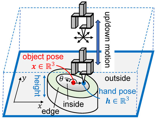
Figure 1.
Problem condition: the robot hand moves either horizontally or vertically; at the bottom plane, the hand can be either inside or outside the object.
One application of this problem is to improve the efficiency of estimating the aperture pose for inserting a hand into a transparent container such as a beaker, which has a relatively small aperture, in order to pick up an object within. The system can accommodate containers with various aperture shapes by collecting observational data offline and constructing a observation model for arbitrary shapes.
2.1. Conditions
The geometrical shape of the object, including its height, is known; however, the reaction force observed by the force sensor at contact with the object is unknown. Thus, the relation should be obtained by experiment. The object is assumed to be rigid and does not deform by contact or move during the estimation process.
2.2. Object Property and Basic Strategy of Contact Motion
Based on the assumptions mentioned above, exploration of the robot hand is designed as a combination of planar motion and up/down motion. In the up-motion plane, the hand can freely move horizontally without any contact. In the down-motion plane, on the other hand, the hand will stop its horizontal motion when the force sensor detects that it has contacted the object.
Because the object edge has a certain thickness, the hand can contact the object at the edge when the hand moves from the upper plane to the bottom plane. It is assumed that the contact at the edge can be detected by the force sensor. When the hand is at the bottom plane, it is either inside or outside the object. We define this discrimination as the discrete state.
2.3. Notation
Let denote the pose of the aperture of the object in the world coordinate system. The force sensor information is denoted by , where n denotes the dimension of the force sensor. The discrete state is denoted by . Let denote the pose of the object in the hand coordinate system. The relation between the hand and the object on the horizontal plane is characterized by a boundary function , as shown in the right panel of Figure 2. The correspondence between discrete state d and is provided as follows:
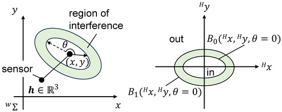
Figure 2.
Boundaries created by edges and apertures on a 2D plane.
3. Estimation of Aperture Based on Discrete State Recognition
An overview of the proposed estimation method is shown in Figure 3. Prior to the estimation, the observation model is constructed as shown in the left frame of the figure. The observation model consists of: (1) the force sensing model; (2) the edge collision model; and (3) the non-existence region model. The first model estimates the object’s pose based on the contact force information obtained during planar exploration and constructs the pose based on samples of and pose collected in the preliminary experiment, where and denote sets of samples with the hand inside and outside the object, respectively, while and denote the respective number of data samples.
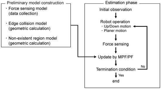
Figure 3.
Method overview.
The second model deals with collisions with the object at the edge during downward motion. During planer exploration, non-contact information can also be utilized to refine the pose estimation, which is realized by the third model. The second and third models are constructed based on the geometric information of the object.
In the estimation phase, shown in the right frame, The initial distribution is generated a priori. An initial distribution is generated under the assumption that an initial visual observation has been obtained. The robot descends to a height at which it can contact an object, then performs a planar motion. Force sensing and updating of the estimated distribution are performed using the method described in the following subsection. While repeating this process, the robot performs up/down motions under certain conditions. The object aperture pose is estimated by the particle filter until it terminates based on a predefined condition. The well-known Kalman Filter expresses the estimated distribution using a Gaussian distribution. In our research, the estimated distribution may be multimodal, making a particle filter more suitable. A histogram filter can also express multimodal distributions; however, the amount of calculation increases when the estimation target becomes high-dimensional. Therefore, both a particle filter (PF) [17,18,19,20,21,22] and manifold particle filter (MPF) [23,24,25] were used for pose estimation, as described in the following sections. The object of pose estimation consists of the following components:
- Particle set with weight and discrete state .
- -
- Set of particles representing object pose:
- -
- Set of weights corresponding to particles:
- -
- Set of discrete states corresponding to particles:
- Non-existence region of object .
Here, denotes the total number of particles and time step is incremented after each exploration action. Each particle has a weight and a discrete state .
3.1. Particle Filter Update for Non-Contact Observation
The PF was applied for pose estimation as depicted in Algorithm 1 in order to reflect non-contact sensing information during planar exploration. In a general PF, particles are sampled based on the state transition probability. In our problem, however, the pose of the object is assumed to be fixed and there is no state transition. Therefore, in our method we use the distribution of the particles at one step prior, without sampling at step 1. The discrete states of the particles are directly inherited from one step prior as well.
| Algorithm 1 Particle filter for non-contact information processing without state transition |
| Input: Particle sets and and sensor observation (non-contact) Output: Particle sets , and 1: {, } 2: weighted by non-contact model 3: Resample |
When the hand has moved along a linear trajectory in the lower plane without force sensation, it means that the object does not exist in the corresponding region when considering the object as a 2D shape. Thus, in the case where the hand moves from to , as shown in Figure 4, the gray region should be omitted from the probability distribution.
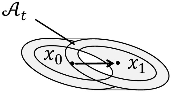
Figure 4.
Non-existence region, as determined by hand motion without force sensation.
The particles are weighted based on the non-contact model . Let denote the non-existence region where no object is supposed to exist based on the non-contact information and the hand motion trajectory, and let denote the set of particles that are located in , with . The weights of particles are reset as follows:
This process corresponds to Step 2 in the algorithm. Because the number of active particles with positive weights decreases during the process, active particles are recovered by resampling at Step 3 while preserving the discrete state .
Note that the estimated non-existence region is accumulated through the process. Let denote the accumulated non-existence region, which is updated using the non-contact motion at time step t as
3.2. Manifold Particle Filter (MPF) with Discrete State Discrimination
When contact is observed by the force sensor, the pose of the object can be constrained on a low-dimensional manifold (surface of the object). Under the original PF framework, particles that are not located on the manifold should be deleted, as they are not consistent with the contact observation. To prevent such particle loss, an MPF directly samples particles from the low-dimensional manifold. Furthermore, the discrete state discrimination as to whether the hand is inside or outside the object when the hand descends is used for pose estimation and the exploration strategy. The MPF algorithm applied to the problem is shown in Algorithm 2.
| Algorithm 2 Manifold particle filter with discrete state discrimination |
| Input: Particle sets , and and sensor observation (contact) Output: Particle sets , and 1: particle sampled from 2: weights calculated by EstimateDensity 3: Resample |
3.2.1. Methods for Updating the Estimated Distribution
At Step 1 in the algorithm, particles are sampled from probability distribution . There are two kinds of contact models: the edge collision model for the hand’s descending motion, and the force sensing model for planar (horizontal) exploration. For construction of the edge model, is constructed by extracting satisfying and the appropriate sensor information .
For the force sensing model, the sample sets and are used to construct . The following procedures are repeated for both cases, and . First, is regressed using a Gaussian process (GP) with a Gaussian kernel. Note that the superscript H is omitted in the following for simplicity of notation. Based on the regression, the average sensor value is determined and is approximated in discrete multi-dimensional grids following the Bayes rule. Suppose that the pose space is discretized into grids with boundary vector and by
Using the mean of the boundary , (with expressed in the hand coordinate) is approximated as follows:
where denotes the set of indices of the grid that is not contained in region .
Because the particles are sampled in the world coordinate, the probability of in (5), which is expressed in the hand coordinate, should be transformed to the world coordinate. Let denote a homogeneous transformation matrix from the world coordinate to the hand coordinate at time step t. Using this transformation, the probability distribution for Step 1 is provided by
Using the distribution, the particles are sampled with discrete state information as and .
Step 2 of Algorithm 2 assigns weights to the set of particles based on the kernel density estimation of particles . EstimateDensity() is represented as
where denotes the parameter matrix used for density estimation.
At Step 3, particles are resampled based on and all weights are reset to while preserving the discrete state . The final output of the algorithm is provided by and , as is uniform with the same weights over the particles.
3.2.2. Usage of Particle Output
The object’s pose is estimated using . Instead of a weighted average over all particles, an estimation (denoted by ) is determined using kernel density estimation, as follows:
The discrete state is then probabilistically estimated from the set of particles after resampling, as follows:
3.3. Exploration Strategy Based on Discrete State
The pseudo-code of the robot operation is depicted in Algorithm 3. Initially, a rough estimation of the object pose is provided and the first target position on the 2D plane is decided according to the initial estimation. When the hand descends to the bottom with the target 2D position, the hand may collide with the object at the edge. In such a case, the distribution is updated by the MPF using the edge collision model . For Update-hand-target( ) at Step 7, is updated by adding random values. Note that the discrete state is not considered in the case of collision during descending motion, as it is defined only when the hand is at the bottom plane during horizontal exploration.
| Algorithm 3 Exploration of hand with pose/discrete state estimation |
| 1: Initialization 2: Set initial particle sets , and based on initial estimation 3: Set initial hand target 4: while true do 5: Descend-hand() 6: if Collision then 7: Update-hand-target( ) 8: Update distribution by MPF 9: else 10: repeat 11: Contact-action( ) 12: Update distribution by MPF/PF 13: if then 14: Update-hand-target( ) 15: break 16: end if 17: until Estimation-convergence( ) 18: end if 19: Raise-hand( ) 20: end while |
When the descent motion is complete, Contact action is executed. In Contact action, the target position of the exploration is determined by the estimated value and the position information of randomly extracted contact data. If the hand contacts the object, the distribution is updated based on the MPF (Algorithm 2), while if the hand finishes the motion without contact, the distribution is updated by the PF (Algorithm 1).
If the hand is expected to be outside the object, then the hand is relocated, aiming at another target 2D position. Equation (12) with the p-th threshold value is used for this judgment. For Update-hand-target( ) at Step 14, in (10) is used. When the robot raises its hand, the discrete state estimation is reset. This is naturally done at Step 1 of Algorithm 2 at the next contact sensing, as the discrete states are sampled based only on the new contact observation. This exploration strategy allows the robot to collect useful contact information more efficiently, thereby improving the efficiency of the pose estimation.
The total exploration and estimation process is finished when the following termination conditions are satisfied:
where represents the moving average of the estimate after the t-th contact action, T is the size of the average, -th is the threshold value, represents the variance of the set of particles, and -th denotes the variance threshold.
4. Experiment
4.1. Condition
A 5-DOF manipulator manufactured by HEBI Robotics [33] was used in the experiment, with a small force sensor manufactured by Touchence [34] mounted on the hand tip. This force sensor is equipped with Micro-Electro-Mechanical Systems (MEMS) to achieve miniaturization. The piezoresistive layer detects force by measuring the change in resistance. The experimental system and force sensor are shown in Figure 5. A force sensor was attached to the center of the hand to obtain contact information and conduct experiments. Grasping would require changing the position of the force sensor, which would not very difficult; however, this is left to future work. This force sensor can measure six axes (fx, fy, fz, Mx, My, Mz); the rated loads are ±7.0 N for fx and fy, 18.0 N for fz, ±15.0 Nmm for Mx and My, and ±10 Nmm for Mz. The resolution is 0.5 N for fx, fy, and fz and 0.2 Nmm for Mx, My, and Mz. The measurement accuracy is ±7.5%, and a measurement cycle of 10 ms was used. The force sensor was connected via spring to a contactor with a length of 30 mm in order prevent any sudden increases in the reaction force. As the rigid bodies came into contact with each other, an elastic body was installed between the sensor and the contact to prevent damage to either the robot or the object.
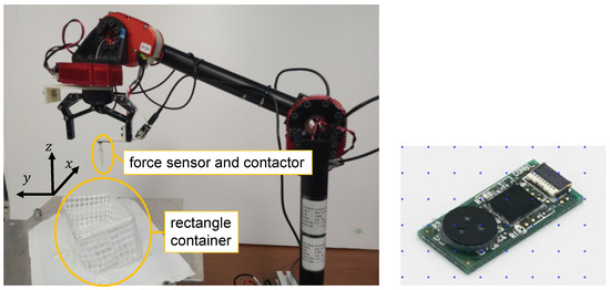
Figure 5.
Experimental system and force sensor.
The objects consisted of a rectangular container 140 mm in length and 85 mm in width, a regular triangle of 160 mm per side, and an irregular quadrangle with the sizes shown in the Figure 6 The heights of the objects were all 65 mm. The pose of the object’s aperture (x, y, and ) in the world coordinate system is denoted by , while the hand pose is denoted by , as the hand is in a constant posture. The robot estimated the aperture pose of the object in the world coordinate system from the hand tip pose calculated from the kinematics of the manipulator and the sensor information .

Figure 6.
Shape of object (left: rectangle; center: regular triangle; right: irregular quadrangle.) Numbers are provided in units of mm.
Initially, the robotic hand was positioned at the origin in the x and y planes and began to move from a height of 195 mm above the steel table. Assuming that the visual sensor can estimate the approximate location of the object, the hand then transitioned to the initial distribution estimates and . After that, the robot executed “Descend hand” with . If the contact condition was met while descending the hand, the robot recognized that it had collided with the edge of the container, executed the estimation process using the MPF as , and moved the hand upward. The contact condition was realized when either fx, fy, or fz became larger than 0.6 N or when either Mx or My became larger than 0.8 Nmm. If the hand was successfully lowered, a contact action was executed. When the contact condition was met, the hand retreated 10 mm in the direction opposite to that of the action, then executed the estimation process using the MPF. If the contact condition could not be satisfied during the action, the hand stopped at the selected position and the estimation process was executed by the PF as . The contact condition was the same as in the above condition. When the MPF was executed, the sensor information s was normalized. The contact action was then executed again from the position at which it stopped for the MPF/PF estimation process, and the contact action was repeated; if the robot recognized that the hand was positioned outside, then it executed “Raise hand” and moved to the estimated value.
Next, was calculated in space with , , ; the total number of grids for discretization was 38,475. The kernel parameters of the kernel were , , and . The variances were determined from the observed data as follows:
where denotes the i-th component of . The number of particles was set to represent the probability distribution in the MPF/PF. The parameter used for kernel density estimation in the MPF was set to . The MPF/PF termination conditions were set as , , and . The robot recognized that convergence was difficult for ; thus, the termination conditions were set to , , and . Moreover, the robot recognized that convergence was very difficult for ; thus, the termination conditions were set to , , and .
The following explanation covers implementation of the non-existence region when the robot executes the t-th contact motion and finds no contact. Let denote the non-existence region of the object at the position of the hand before the contact motion. Let denote the non-existence region of the object at the position of the hand where the hand moves l[mm] horizontally. If the total moving distance is L [mm], then the non-existence area is as follows:
Here, were determined by the size and posture of each of the three objects and the moving distance l of the hand.
To verify the effectiveness of the proposed method, we experimented with two methods that did not discriminate between the discrete states. In the first “SD:stay-down” method the hand descends one time, then contact search is executed using only horizontal movements. When the hand descends to the outside of the container, there is no inside transition; if the hand descends to the inside of the container, then there is no raising or lowering of the hand. In the second “LR:lift-random” method, the hand is raised with a probability of 1/2 for each contact action, then descends to the estimated value. The proposed method (DSB:discrete state-based lift strategy) raises the hand when the discrete state is recognized as outside, then lowers the hand to the estimated value. The threshold for recognition as outside was set to .
4.2. Preliminary Experiment for Building the Contact Model
In the preliminary experiment, the true pose of the object’s aperture was known and samples of the input and output were collected. Contact samples were collected from both inside and outside the objects. In the former case, the hand was set to start at the center of gravity of the aperture at a height that would allow the contactor to contact the rectangular container edge. The robot moved horizontally in the direction of angle along the x-axis, and samples of and were collected at the time of contact. Contact information was obtained at 36 positions with . To collect samples from outside the objects, the hand was set to start at a position of 90 mm in the direction of from the center of gravity of the aperture at a height that allowed the contactor to contact the edge of the rectangular container. The samples of and were collected at the time of contact by horizontal movement toward the position of the aperture’s center of gravity. As in the case of contact from the inside, was set to obtain the contact information at 36 positions. The robot was required to obtain contact samples from different postures in a rectangular container. In this case, the sample was collected by changing the joint angle of the fifth axis of the manipulator () while maintaining the fixed posture of the container. The experiment was conducted assuming and 18 posture patterns of the container. A total of 36 × 18 × 2 = 1296 inside and outside samples were collected. For the regular triangular object, the experiment was conducted assuming and 12 posture patterns of the container. Therefore, a total of 36 × 12 × 2 = 864 inside and outside samples were collected. Due to the lack of symmetry, for the irregular quadrangle object the experiment was conducted assuming and 36 posture patterns of the container. Therefore, a total of 36 × 36 × 2 = 2592 inside and outside samples were collected.
4.3. Results
The experimental results for the three types of objects are shown in Table 1, Table 2 and Table 3. In the tables, and denote the total number of contact actions and the operation time until the termination condition was satisfied. The errors of the convergence values of the estimation were ,,. We experimented ten times with and for the true pose of the rectangular container five times each. For regular triangular objects, the true pose was and . For irregular quadrilateral objects, the true pose was and . The initial distribution was changed in all ten experiments. The results for rectangular objects are described below. The robot was able to perform estimation with an average error of less than 15 degrees and an average positional error of less than 7 mm. Comparison of the operation times shows that the DSB method is the most efficient, followed by the SD and LR methods. The DSB method has a smaller variance than both other methods, indicating that its estimation efficiency was more stable. The errors for the regular triangular objects were slightly larger than those for the rectangular objects; however, the superiority of the results with respect to the estimation efficiency remained the same. The posture error was larger in the case of irregular quadrangular objects. The operation time was shorter for SD than for DSB. Finally, the irregular quadrangle objects required more contact motions to converge.

Table 1.
Results of the discrete state-based lift strategy (DSB), stay-down method (SD), and lift-random method (LR) on the rectangular object.

Table 2.
Results of the discrete state-based lift strategy (DSB), stay-down method (SD), and lift-random method (LR) on the regular triangle object.

Table 3.
Results of the discrete state-based lift strategy (DSB), stay-down method (SD), and lift-random method (LR) on the irregular quadrangle object.
Figure 7 shows the updated distribution for the experiment with DSB and the distribution satisfying the termination condition. The initial distribution was artificially generated under the assumption that it was obtained from visual sensors. The robot descended its hand to the estimated initial distribution and moved to contact, but was unable to contact the object. The result of updating the distribution from the non-contact information using the particle filter is represented as . Compared to the initial distribution, resampling that considers non-existence regions shows that the distribution of the particles is missing. In the next contact action, the robot contacted the container and sampled particles from the observation model. Here, the blue particles have “out” information and the red particles have “in” information. Kernel density estimation was based on the distribution of X(1) results in regions where particles were present with a large weight, and particles close to these regions were resampled. Because the discrete state estimate resulted in p(d=out) = 1, the robot raised the hand and descended to the estimated position, causing the hand to transition to the inside of the container. After three repeated contact actions, the estimates converged and the robot stopped operating. The variance of in the converged is relatively large, which is discussed in the next subsection.
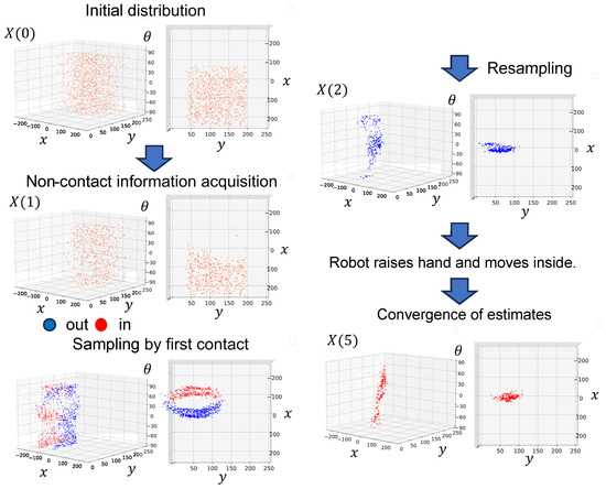
Figure 7.
Updating from the initial distribution X (0) to X (1) with non-contact information. The distribution sampled at the next contact is represented in the lower left corner. This sampled distribution was resampled by weighting by X (1) and updating to X (2). The contact action was then repeated, ultimately converging to the X (5) distribution.
Figure 8 shows the results of updating the distribution using the MPF from the third to the fifth contact information in the experiment with the SD strategy. Under SD, when the hand descends to the outside of the container, it does not transition to the inside, and often repeats the contact at the same position. In this case, the sampled distributions are similar, and the distributions for weighting are similar as well; therefore, the estimates and variances do not change significantly when the distributions are updated. Therefore, the contact action must be repeated many times before convergence is achieved, which degrades the estimation efficiency.
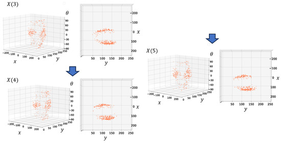
Figure 8.
Distribution updated using the SD method with three contact actions. The distribution did not change significantly because of repeated contacts at similar positions.
Table 4 shows the number of times the hand up/down motion was performed during the ten experiments for the LR strategy along with the average number of such motions. DSB often required only one up/down motion when the hand descended outside the container based on the estimated initial distribution. However, because this method did not discriminate between the discrete states and could not determine whether the hand was inside or outside the container, the robot performed an average of 4.4 hand up/down motions. As shown in Figure 9, the robot often made up/down motions with the hand even when the hand was positioned inside, resulting in wasted operation time. On the other hand, owing to stochastic up/down motions, estimation was sometimes completed in a short time, leading to a large variance in the total operation time. Because this up/down motion represents a combination of linear motions, the total motion time can be optimized by designing the program to perform circular motions; however, the superiority of the results compared to the proposed method would not change.

Table 4.
Number of up/down motions.

Figure 9.
Inside-to-inside transition using the LR method.
4.4. Discussion
Figure 10 shows the kernel density-estimated distribution of only the component of particles sampled at the last contact before convergence (shown in Figure 7). This figure shows one large peak at approximately −60 and a slightly smaller peak at approximately 30. When the postures of the rectangular container are 30 and −60, as shown in Figure 11, the robot cannot distinguish these two postures from the force information when contacting the edge indicated by the arrow from the inside. For this reason, the distribution of the component of the particles sampled from the observation model became multimodal even though the true posture of the object was 30, causing the variance of the updated distribution to increase. If the object has a characteristic shape at the aperture and the sensor can obtain observation information that reflects this characteristic, then the variance of can be reduced.
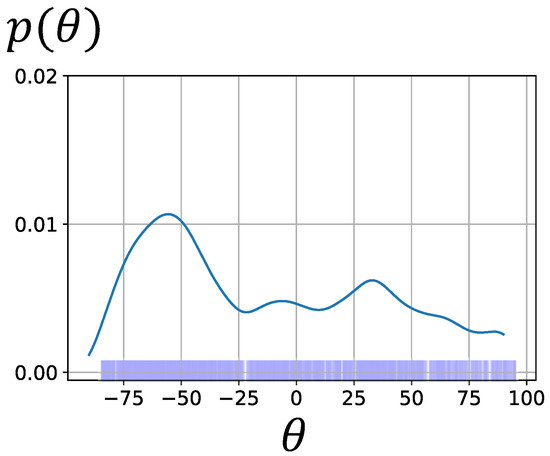
Figure 10.
Representation of the distribution of sampled particles with kernel density estimation of only the component.
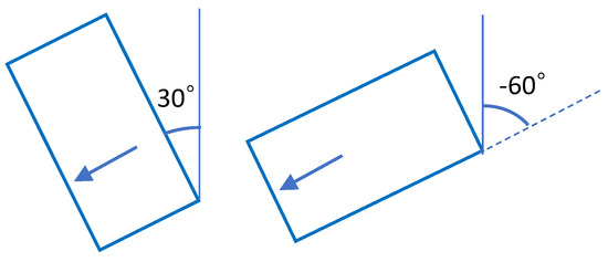
Figure 11.
The robot cannot distinguish whether the posture is 30 or −60 degrees using only the contact information.
Figure 12 shows the progress of the particle distribution over five contact actions in an experiment with the SD strategy. This experiment satisfied the termination condition, as the estimates converged after five contact motions. Based on the initial distribution, the hand descended outside the container; the randomness of the contact action allowed the robot to search a wide region, providing useful contact/non-contact information to refine the estimate. The current contact motion selection is effective when the hand is positioned inside the container; coincidentally, however, this result also worked well when the hand was positioned outside the container. Based on this result, efficient estimation can be achieved by selecting a contact motion that searches a large region when the hand is positioned outside the container. In such cases, discrete state estimation is necessary because the action strategy can differ from that of the inside case.

Figure 12.
Distribution with fast convergence using the SD method.
Figure 13 shows the transition of the variance of by repeated contact motions in one experiment with each object. For the irregular quadrangle object, the variance of decreased after the eighth contact motion, although it was larger than that of the other objects. This is because the four posture patterns could not be distinguished from the sensor information, as shown in Figure 14. Therefore, the experiment with irregular quadrangles required a large number of contact motions, resulting in a large error in .
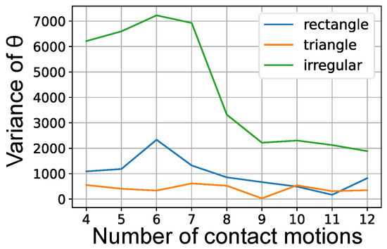
Figure 13.
Four posture patterns of irregular quadrangular objects.
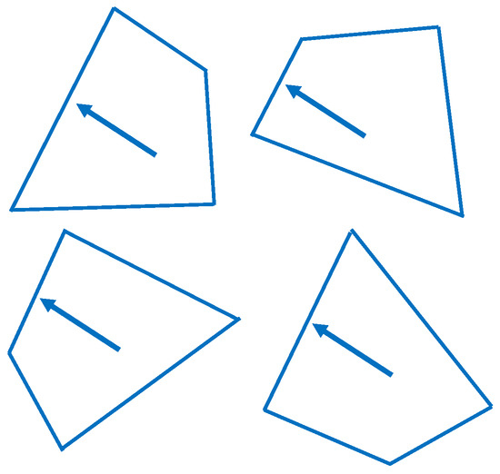
Figure 14.
Variance of with respect to the number of contact movements.
The experimental results for irregular quadrilateral objects showed smaller operation times for SD than for DSB. In the case of SD, the robot repeatedly performs contacts from the outside in a similar position, resulting in a shorter operating distance and shorter operating time. However, this requires a greater number of contact motions than the DSB strategy. In the experiment with irregular quadrilateral objects, about 45 s was required for one contact information processing calculation, compared to about 15 s for one non-contact information processing calculation. Therefore, it is more important to reduce the number of contact motions than the operation time.
5. Conclusions
To realize the task of inserting a robotic hand into a container, the pose of the aperture was estimated using a probabilistic state estimation method. In the case of rectangular and regular triangular objects, the following conclusions were obtained. Although the estimation error of the posture was sometimes large, the robot was able to estimate with an average error of less than 17 degrees and an average positional error of less than 13 mm. With this accuracy, the hand can be inserted close to the center of gravity of the container aperture. In the proposed method, the robot estimates the discrete positional relationship between the hand and container and selects the action according to the discrete state, thereby improving the estimation efficiency. Compared with other methods, the proposed method was superior in terms of the number of contact motions and total operation time. Furthermore, the proposed method showed stable estimation efficiency with small variance in the number of contact motions and total operation time. Although the experiment with irregular objects resulted in a larger estimation error for , the superiority of the proposed method remained clear. Even with the proposed method, at least one up-down motion is required when the contact motion is started from the outside, and at least five contacts are required. It would be possible to achieve more efficient estimation by changing the hardware, for instance by increasing the number of force sensors.
The SD method repeats contact actions from outside the container, and the estimation sometimes converged after a small number of contact motions. This means that if a strategy involving contact action from outside the container were properly designed, it could provide efficient estimates without needing to transition to the inside. In this case, it would be necessary to estimate the discrete state in which the hand was positioned outside the container, further highlighting the superiority of the proposed method. In future work, we would like to verify our proposed system with an object featuring a deformable aperture, such as a bag, and to utilize a sensor that can acquire rich information. By integrating the visual and tactile senses, it should be possible to realize more accurate and shorter estimation times for transparent bags. When the aperture exists in a three-dimensional space, the pose representation becomes a high-dimensional vector, and the total number of particles used in the estimation method must be increased. In principle, it would be possible to increase the dimensionality in the proposed system, although a method for reducing the amount of calculation would be required. Although we estimated the pose in this paper through a wide range of contacts with the object, it would also be possible to estimate the pose in a partial space that allows the hand to be inserted, potentially reducing the amount of calculation.
Author Contributions
The contributions of each author are listed as follows: D.K. devised the methodology, designed the software, conducted the experiments, and wrote the paper; Y.K. provided extensive suggestions and advice on problem definition, methodology, and experiments, and provided guidance in writing the paper; D.T. assisted with the experiments; N.M., K.H. and D.U. provided advice from an application perspective. All authors have read and agreed to the published version of the manuscript.
Funding
This research received no external funding.
Informed Consent Statement
Not applicable.
Data Availability Statement
Dataset available on request from the authors.
Acknowledgments
We appreciate the members of our laboratory at Shizuoka University.
Conflicts of Interest
The funders had no role in the design of the study; in the collection, analyses, or interpretation of data; in the writing of the manuscript; or in the decision to publish the results.
Abbreviations
The following abbreviations are used in this manuscript:
| PF | Particle Filter |
| MPF | Manifold Particle Filter |
| DSB | Discrete State-Based |
| SD | Stay-Down |
| LR | Lift-Random |
References
- Changhyun, C.; Yuichi, T.; Oncel, T.; Ming-Yu, L.; Srikumar, R. Voting-based pose estimation for robotic assembly using a 3D sensor. In Proceedings of the IEEE International Conference on Robotics and Automation (ICRA), St Paul, MN, USA, 14–18 May 2012; pp. 1724–1731. [Google Scholar] [CrossRef]
- Choi, C.; Christensen, H.I. 3d pose estimation of daily objects using an rgb-d camera. In Proceedings of the IEEE/RSJ International Conference on Intelligent Robots and Systems (IROS), Vilamoura-Algarve, Portugal, 7–12 October 2012; pp. 3342–3349. [Google Scholar] [CrossRef]
- Aldoma, A.; Marton, Z.C.; Tombari, F.; Wohlkinger, W. Tutorial: Point cloud library: Three-dimensional object recognition and 6 dof pose estimation. IEEE Robot. Autom. Mag. 2012, 19, 80–91. [Google Scholar] [CrossRef]
- Krull, A.; Brachmann, E.; Michel, F.; Yang, M.Y.; Gumhold, S.; Rother, C. Learning Analysis-by-Synthesis for 6D Pose Estimation in RGB-D Images. In Proceedings of the IEEE International Conference on Computer Vision, Santiago, Chile, 7–13 December 2015; pp. 954–962. [Google Scholar] [CrossRef]
- Xiang, Y.; Schmidt, T.; Narayanan, V.; Fox, D. Posecnn: A convolutional neural network for 6d object pose estimation in cluttered scenes. arXiv 2017, arXiv:1711.00199. [Google Scholar] [CrossRef]
- Wang, C.; Xu, D.; Zhu, Y.; Martin-Martin, R.; Lu, C.; Fei-Fei, L.; Savarese, S. Densefusion: 6D object pose estimation by iterative dense fusion. In Proceedings of the IEEE Conference on Computer Vision and Pattern Recognition, Long Beach, CA, USA, 15–20 June 2019; pp. 3338–3347. [Google Scholar]
- Sundermeyer, M.; Durner, M.; Puang, E.Y.; Marton, Z.C.; Vaskevicius, N.; Arras, K.O.; Triebel, R. Multi-Path Learning for Object Pose Estimation Across Domains. In Proceedings of the 2020 IEEE/CVF Conference on Computer Vision and Pattern Recognition (CVPR), Seattle, WA, USA, 14–19 June 2020; pp. 13913–13922. [Google Scholar] [CrossRef]
- Han, K.; Wang, Y.; Chen, H.; Chen, X.; Guo, J.; Liu, Z.; Tang, Y.; Xiao, A.; Xu, C.; Xu, Y.; et al. A Survey on Vision Transformer. IEEE Trans. Pattern Anal. Mach. Intell. 2023, 45, 87–110. [Google Scholar] [CrossRef] [PubMed]
- Anzai, T.; Takahashi, K. Deep Gated Multi-modal Learning: In-hand Object Pose Changes Estimation using Tactile and Image Data. In Proceedings of the IEEE/RSJ International Conference on Intelligent Robots and Systems, Las Vegas, NV, USA, 25–29 October 2020; pp. 9361–9368. [Google Scholar] [CrossRef]
- Bimbo, J.; Kormushev, P.; Althoefer, K.; Liu, H. Global estimation of an object’s pose using tactile sensing. Adv. Robot. 2015, 29, 363–374. [Google Scholar] [CrossRef]
- Bauzá, M.; Valls, E.; Lim, B.; Sechopoulos, T.; Rodriguez, A. Tactile Object Pose Estimation from the First Touch with Geometric Contact Rendering. In Proceedings of the Conference on Robot Learning, Virtual, 16–18 November 2020. [Google Scholar]
- Donlon, E.; Dong, S.; Liu, M.; Li, J.; Adelson, E.H.; Rodriguez, A. GelSlim: A High-Resolution, Compact, Robust, and Calibrated Tactile-sensing Finger. arXiv 2018, arXiv:1803.00628. [Google Scholar]
- Taylor, I.H.; Dong, S.; Rodriguez, A. GelSlim 3.0: High-Resolution Measurement of Shape, Force and Slip in a Compact Tactile-Sensing Finger. In Proceedings of the 2022 International Conference on Robotics and Automation (ICRA), Philadelphia, PA, USA, 23–27 May 2022; pp. 10781–10787. [Google Scholar] [CrossRef]
- Pfanne, M.; Chalon, M.; Stulp, F.; Albu-Schäffer, A. Fusing Joint Measurements and Visual Features for In-Hand Object Pose Estimation. IEEE Robot. Autom. Lett. 2018, 3, 3497–3504. [Google Scholar] [CrossRef]
- Wang, J.; Wilson, W. 3D relative position and orientation estimation using Kalman filter for robot control. In Proceedings of the 1992 IEEE International Conference on Robotics and Automation (ICRA), Nice, France, 12–14 May 1992; Volume 3, pp. 2638–2645. [Google Scholar] [CrossRef]
- Morency, L.P.; Sundberg, P.; Darrell, T. Pose estimation using 3D view-based eigenspaces. In Proceedings of the IEEE International SOI Conference, Nice, France, 17 October 2003; pp. 45–52. [Google Scholar] [CrossRef]
- Kitagawa, G. Monte Carlo Filter and Smoother for Non-Gaussian Nonlinear State Space Models. J. Comput. Graph. Stat. 1996, 5, 1–25. [Google Scholar] [CrossRef]
- Álvarez, D.; Roa, M.A.; Moreno, L. Tactile-Based In-Hand Object Pose Estimation. In Proceedings of the Third Iberian Robotics Conference, Seville, Spain, 22–24 November 2017; Volume 694, pp. 716–728. [Google Scholar]
- Zhang, L.; Trinkle, J.C. The application of particle filtering to grasping acquisition with visual occlusion and tactile sensing. In Proceedings of the IEEE International Conference on Robotics and Automation(ICRA), St Paul, MN, USA, 14–18 May 2012; pp. 3805–3812. [Google Scholar] [CrossRef]
- Drigalski, F.; Taniguchi, S.; Lee, R.; Matsubara, T.; Hamaya, M.; Tanaka, K.; Ijiri, Y. Contact-based in-hand pose estimation using Bayesian state estimation and particle filtering. In Proceedings of the 2020 IEEE International Conference on Robotics and Automation (ICRA), Paris, France, 31 May–31 August 2020; pp. 7294–7299. [Google Scholar] [CrossRef]
- Drigalski, F.; Hayashi, K.; Huang, Y.; Yonetani, R.; Hamaya, M.; Tanaka, K.; Ijiri, Y. Precise Multi-Modal In-Hand Pose Estimation using Low-Precision Sensors for Robotic Assembly. In Proceedings of the 2021 IEEE International Conference on Robotics and Automation (ICRA), Xi’an, China, 30 May–5 June 2021; pp. 968–974. [Google Scholar] [CrossRef]
- Miyazawa, N.; Kato, D.; Kobayashi, Y.; Hara, K.; Usui, D. Optimal action selection to estimate the aperture of bag by force-torque sensor. Adv. Robot. 2024, 38, 95–111. [Google Scholar] [CrossRef]
- Koval, M.C.; Dogar, M.R.; Pollard, N.S.; Srinivasa, S.S. Pose estimation for contact manipulation with manifold particle filters. In Proceedings of the 2013 IEEE/RSJ International Conference on Intelligent Robots and Systems, Tokyo, Japan, 3–7 November 2013; pp. 4541–4548. [Google Scholar] [CrossRef]
- Koval, M.C.; Klingensmith, M.; Srinivasa, S.S.; Pollard, N.S.; Kaess, M. The manifold particle filter for state estimation on high-dimensional implicit manifolds. In Proceedings of the 2017 IEEE International Conference on Robotics and Automation (ICRA), Singapore, 29 May–3 June 2017; pp. 4673–4680. [Google Scholar]
- Yagi, H.; Kobayashi, Y.; Kato, D.; Miyazawa, N.; Hara, K.; Usui, D. Object Pose Estimation Using Soft Tactile Sensor Based on Manifold Particle Filter with Continuous Observation. In Proceedings of the IEEE/SICE International Symposium on System Integration, Atlanta, GA, USA, 17–20 January 2023; pp. 1–6. [Google Scholar]
- Ichiwara, H.; Ito, H.; Yamamoto, K.; Mori, H.; Ogata, T. Contact-Rich Manipulation of a Flexible Object based on Deep Predictive Learning using Vision and Tactility. In Proceedings of the 2022 International Conference on Robotics and Automation (ICRA), Philadelphia, PA, USA, 23–27 May 2022; pp. 5375–5381. [Google Scholar] [CrossRef]
- Ningquan, G.; Zhizhong, Z.; Ruhan, H.; Lianqing, Y. ShakingBot: Dynamic manipulation for bagging. Robotica 2024, 42, 1–17. [Google Scholar] [CrossRef]
- Hebert, P.; Howard, T.; Hudson, N.; Ma, J.; Burdick, J.W. The next best touch for model-based localization. In Proceedings of the 2013 IEEE International Conference on Robotics and Automation (ICRA), Karlsruhe, Germany, 6–10 May 2013; pp. 4673–4680. [Google Scholar] [CrossRef]
- B. Saund, S.C.; Simmons, R. Touch based localization of parts for high precision manufacturing. In Proceedings of the 2017 IEEE International Conference on Robotics and Automation (ICRA), Singapore, 29 May–3 June 2017; pp. 378–385. [Google Scholar] [CrossRef]
- Wang, S.; Wu, J.; Sun, X.; Yuan, W.; Freeman, W.T.; Tenenbaum, J.B.; Adelson, E.H. 3D Shape Perception from Monocular Vision, Touch, and Shape Priors. In Proceedings of the 2018 IEEE/RSJ International Conference on Intelligent Robots and Systems (IROS), Madrid, Spain, 1–5 October 2018; pp. 1606–1613. [Google Scholar]
- Yi, Z.; Calandra, R.; Veiga, F.; van Hoof, H.; Hermans, T.; Zhang, Y.; Peters, J. Active tactile object exploration with Gaussian processes. In Proceedings of the 2016 IEEE/RSJ International Conference on Intelligent Robots and Systems (IROS), Daejeon, Republic of Korea, 9–14 October 2016; pp. 4925–4930. [Google Scholar] [CrossRef]
- Kato, D.; Kobayashi, Y.; Miyazawa, N.; Hara, K.; Usui, D. Efficient Sample Collection to Construct Observation Models for Contact-Based Object Pose Estimation. In Proceedings of the 2024 IEEE/SICE International Symposium on System Integration (SII), Ha Long, Vietnam, 8–11 January 2024; pp. 922–927. [Google Scholar] [CrossRef]
- HEBI Robotics. Available online: https://hebirobotics.com/ (accessed on 10 August 2022).
- Shokac Cube. Available online: http://touchence.jp/en/products/cube.html (accessed on 10 August 2022).
Disclaimer/Publisher’s Note: The statements, opinions and data contained in all publications are solely those of the individual author(s) and contributor(s) and not of MDPI and/or the editor(s). MDPI and/or the editor(s) disclaim responsibility for any injury to people or property resulting from any ideas, methods, instructions or products referred to in the content. |
© 2024 by the authors. Licensee MDPI, Basel, Switzerland. This article is an open access article distributed under the terms and conditions of the Creative Commons Attribution (CC BY) license (https://creativecommons.org/licenses/by/4.0/).