A Novel Actor—Critic Motor Reinforcement Learning for Continuum Soft Robots

Abstract

Reinforcement learning (RL) is explored for motor control of a novel pneumatic-driven soft robot modeled after continuum media with a varying density. This model complies with closed-form Lagrangian dynamics, which fulfills the fundamental structural property of passivity, among others. Then, the question arises of how to synthesize a passivity-based RL model to control the unknown continuum soft robot dynamics to exploit its input–output energy properties advantageously throughout a reward-based neural network controller. Thus, we propose a continuous-time Actor–Critic scheme for tracking tasks of the continuum 3D soft robot subject to Lipschitz disturbances. A reward-based temporal difference leads to learning with a novel discontinuous adaptive mechanism of Critic neural weights. Finally, the reward and integral of the Bellman error approximation reinforce the adaptive mechanism of Actor neural weights. Closed-loop stability is guaranteed in the sense of Lyapunov, which leads to local exponential convergence of tracking errors based on integral sliding modes. Notably, it is assumed that dynamics are unknown, yet the control is continuous and robust. A representative simulation study shows the effectiveness of our proposal for tracking tasks.

1. Introduction

The essential feature of RL is that it provides a reinforcement signal based on the value function evaluation to compute the present action aiming to learn a task. Such a brief statement deploys a powerful motor learning paradigm [1] from control application through the Actor–Critic scheme, well substantiated by adaptive dynamic programming [2], and optimal control [3] schemes. Recently, model-based (regressor) adaptive and model-free (neural networks) controls have been proposed to deal with uncertainty [4,5,6].

Conventional RL schemes typically require state and action space exploration, demanding massive trials and data to tune and test the system in broad operational conditions. It makes conventional RL an option for some software applications, but are risky for hardware systems. Then, it has been claimed that further research is needed to introduce explicit stability bounds and clear implementation procedures to implement RL schemes for a physical system, such as a robot. However, a distinct feature of the RL massive literature is lack of stability conditions [7], with few exceptions. Then, translational research is required to yield a novel RL scheme with stability analysis, particularly for highly nonlinear systems such as robots, but stability is definitively a requirement for uncertain and disturbed complex deformable (soft body) robots.

We are interested in the particular class of pneumatic-driven continuum soft robots. For these robots, implementing a conventional RL is prone to failure when attempting to operate it away from its narrow operational margin, thus requiring novel RL designs equipped with stability analysis. The stability analysis does not represent a nuisance, unnecessary design requirement, or an elegant, irrelevant usage of mathematics; by contrast, stability is tantamount to guaranteeing the operation of the systems under certain conditions. Thus, stability analysis is required for any novel motor control scheme for nonlinear uncertain models, such as continuum soft robots. Given that RL aims at computing the present action that yields the desired state of a system at a given cost, computational architectures have been studied to explore to state-action space, which has led to software architectures rather than RL’s stability conditions. Thus, large batches of trials, even millions, are regularly carried out for a particular system until it learns the task and a particular set of discrete admissible controls. However, when such a system is a physical entity, like a robot, there is no room for such trials, but it must operate within stability margins. The trial-and-error mechanistic approach of RL tuning is forbidden for robots since fatal failure may arise. Unfortunately, stability requirements for RL applications for robots have not permeated into the computational RL community; better phrased, why does the immense majority of RL literature lack stability? It is worrisome that this fact is not a worry, but rather the norm, in the practice of RL for robots [7], including for deformable (soft) robots [8]. Although the early approaches of RL dynamical systems are used, the principal developments in recent years have improved the algorithms on a finite set of states and controls.

Nonetheless, RL has an enormous advantageous prevalence over “conventional” control in the sense that RL deals with two metrics (performance index and tracking error) while conventional control deals with only one metric (tracking error). RL evaluates performance to issue a reinforced signal to the action (control), which seems very interesting for novel systems, such as the continuum soft robot subject to varying density and a non-constant center of mass [9]. Then, the question arises of how to design a sound (stability-based) RL scheme considering its deformation, which is the essential feature that distinguishes it against conventional rigid-body robots.

In this paper, we entertain the explicit need for rigorous stability of a model-free RL scheme for continuum soft robots [9], where reward evaluates continuous deformation coordinates. Our proposed scheme is similar to adaptive neurocontrol away from optimal-like control. However, it differs from the former because a second neural network (the Critic or Critic NN) aims to enforce the asymptotic stability of the temporal difference error equation in continuous time. Additionally, a so-called Actor NN aims at inverse dynamics compensation. This scheme is called the Actor–Critic Learning of Motor Control. Unlike traditional Actor–Critic schemes [10,11], novel adaptive mechanisms are introduced for neural weights that allows tightly and complex intertwined nonlinear Actor–Critic neural architectures to emerge, substantiated by the closed-loop stability analysis for tracking tasks of the uncertain continuum 3D soft robot subject to Lipschitz disturbances.

Contribution and Organization

The contribution amounts to a novel RL scheme for a novel continuum soft robot [9], using a particular actuation topology [12]. RL’s relevant role evaluation performance is exploited to reinforce the neurocontroller based on the approximation of Bellman’s temporal difference. It represents the accumulated reward-based value function, approximated by the Critic NN using a novel adaptive mechanism of weights with nonlinear neural activations, while the Actor NN compensates approximately for inverse dynamics. A chatterless integral sliding mode is introduced to guarantee error tracking [13]. Overall, tracking with performance evaluation is guaranteed, assuming no knowledge of complex dynamics subject to disturbances, yet with a smooth control action.

This manuscript is organized as follows. Section 2 introduces the preliminaries and problem statement. Section 3 presents the RL design, with stability analysis in the Appendix. Simulations are presented in Section 4 for a 3D continuum soft robot motion tracking an aggressive trajectory, with discussions of the overall scheme presented in Section 5. Finally, concluding remarks are given in Section 6, addressing some advantages and concerns of the proposed scheme.

2. Preliminaries and Problem Statement

Interestingly, there exist hundreds of papers indexed in the academic metasearch engine Scopus under the keywords RL and soft robot addressing a variety of RL implementations to non-rigid-body systems; however, only 24 papers deal precisely with soft-robots; only two mention stability [14,15]; yet, none included any formal stability analysis. Though this amazing body of literature is rapidly changing and will hopefully soon be address stability, this situation speaks for itself about the significant worldwide effort to exploit the powerful characteristics of RL to soft robots. However, it also shows that the solid foundations of RL are taken for granted for novel applications; for example, it meets the theoretical assumptions of the original approach, but is without any rigor to study the subtleties on how to include the differences of each novel system with stability. Not only that, but stability analysis also paves the way to substantiate a specific design within the specificities of each new system; that is, stability analysis tailors the design according to what a particular system is. The result is an efficient RL custom design for the system under study, not a general design for a particular system, which typically leads to conservative and inefficient RL designs. Overall, this brief literature assessment shows the tendency of RL implementations to a large class of systems, including deformable-body robots. This approach limits and weakens its effectiveness since, in practice, each new system differs in many aspects from the ideal one considered initially. Impressive empirical results of the literature empower RL as a viable option worth studying; however, its prime will be highlighted, arguably, when synthesized through stability analysis to deliver an asymptotically stable RL approach for a specific system.

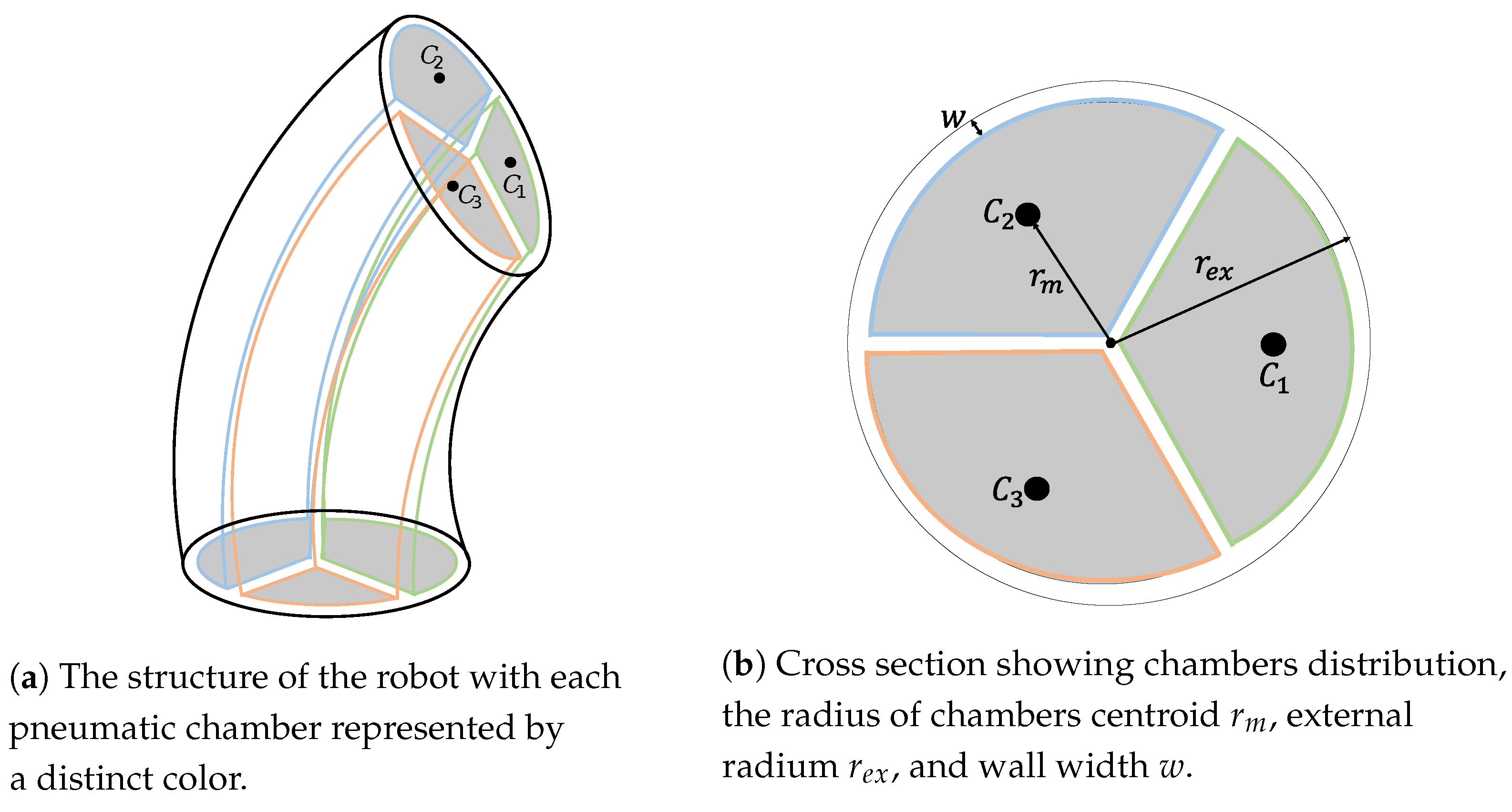
2.1. On Continuum Soft Robots

Soft robots can be classified by their actuation into four types [16]:

• Fluidic Elastomer soft robots (FESRs): This type of soft robots has pneumatic/hydraulic chambers embedded into their bodies, which induce body deformation when pressurized. It can generate movements such as bending, elongation, torsion, and a combination of these movements. For example, the STIFF-FLOP comprises a series of identical elastomeric soft actuators with internal pneumatic chambers to unlock three-dimensional movement and a central chamber for stiffness variation via granular interference phenomena [17].
• Cable-driven soft robots (CDSRs): The robot has external or internal cables that generate deformation by tension variation. However, the type of movement and workspace depend on the number and position of cables, which means that there are more control inputs and rigid elements where cables pivot. Furthermore, the exerted force of this type of actuator depends directly on cables tension and not on stiffness. An example is depicted in [18], where a four-cable-driven soft arm is presented.
• Shape-memory polymer soft robots (SMPSRs): This type encompasses robots composed of polymers with a thermally induced effect, which allows them to go from an initial state to a deformed state. However, SMPSRs do not produce high strain and are usually applied when small deformations are required.
• Dielectric/electroactive polymer soft robots (D/EPSRs): This type of robots are based on deformation phenomena in response to electricity. However, due to their high voltage amplification, their doped elastomer is the most disadvantageous and risky option.

By comparing the actuation mechanisms of these types of soft robots, it is recognized that FESRs have the best relationship between applied force and deformation, given that applied energy (either pneumatic or hydraulic) continuously deforms the elastomer, translating into viscoelastic forces of continuum media, i.e., a change in the distance between each pair of particles in the material. On the other hand, there are three types of morphologies for soft robots that show continuous deformation [19]:

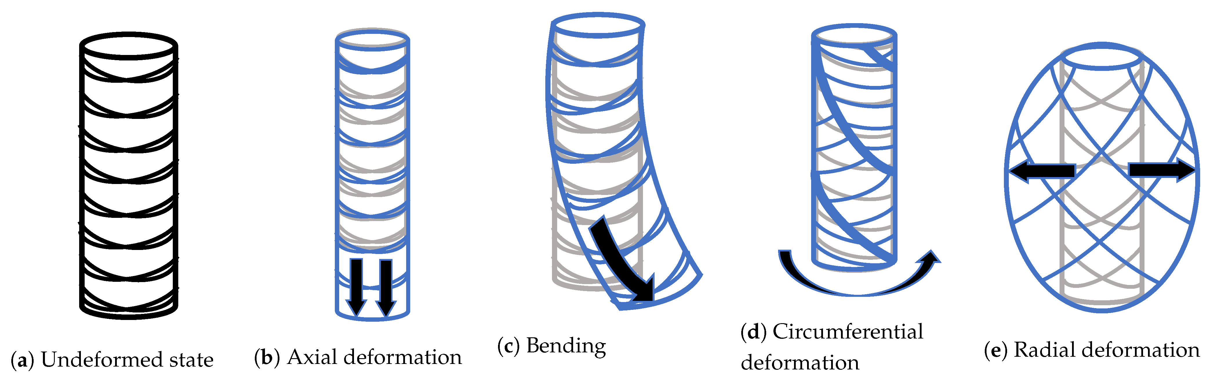
• Cylindrical morphology: The robot’s body is shaped like a cylinder of elastomeric material, with pressure inputs (chambers) radially distributed along an internal radius. When a chamber is pressurized, the body presents a controlled curvature along the extensible center of the robot. Usually, this morphology is built using inextensible braided threads to mitigate radial and circumferential deformations so that the robot’s configuration can be approximated with a minimum set of linearly independent variables principally used as control inputs actuated by pneumatic chambers.
• Ribbed morphology: The robot is composed of three elastomer-based layers. The top and bottom layers have internal ribbed-like structures with multiple rectangular channels connected to fluid transmission lines, whereas the middle layer is a flexible but inextensible restriction. In an active state, where fluid pressurizes a group of chambers, bending is produced. An example is presented in [20] with a soft arm of six ribbed-like segments designed as a manipulation system.
• Pleated morphology: Consists of discrete sections (plates) of elastomeric materials evenly distributed and separated by gaps. At the bottom part, a high-stiffness silicon layer is used to work as an inextensible restriction. Additionally, the top part has hollow cavities (in each plate) connected to a central chamber. When it gets pressurized, each plate experiences balloon-like deformations translated into bending of the high-stiffness silicon layer along the direction of the layer with lower stiffness. An example is presented in [21], where a soft manipulator has six segments with cylindrical cavities, and a pleated-shaped soft gripper is used for grasping purposes.

Among these morphologies, the cylindrical morphology is the one that allows to approximate robot’s deformation through a finite number of variables due to the radial distribution of their pressure entries while simultaneously allowing relatively easy characterization of their geometric variables. Additionally, four types of movement can be distinguished [22]: axial (elongation and retraction of length; see Figure 1b), bending (see Figure 1c), circumferential (translated as torsion; see Figure 1d) and radial (expansion and contraction of cross-sectional area; see Figure 1e). Notice that these movements are achieved by imposing different deformation restrictions.

Thus, we consider in this paper the soft robot defined as a cylindrical-shaped soft body composed of elastomeric material moving from continuous controlled body deformation. Moreover, we refer to a continuum soft robot as a soft robot with continuous infinitesimal deformation of the distance between their particles, and it must not be confused with what was referred to as a continuum robot 20 years ago [23].

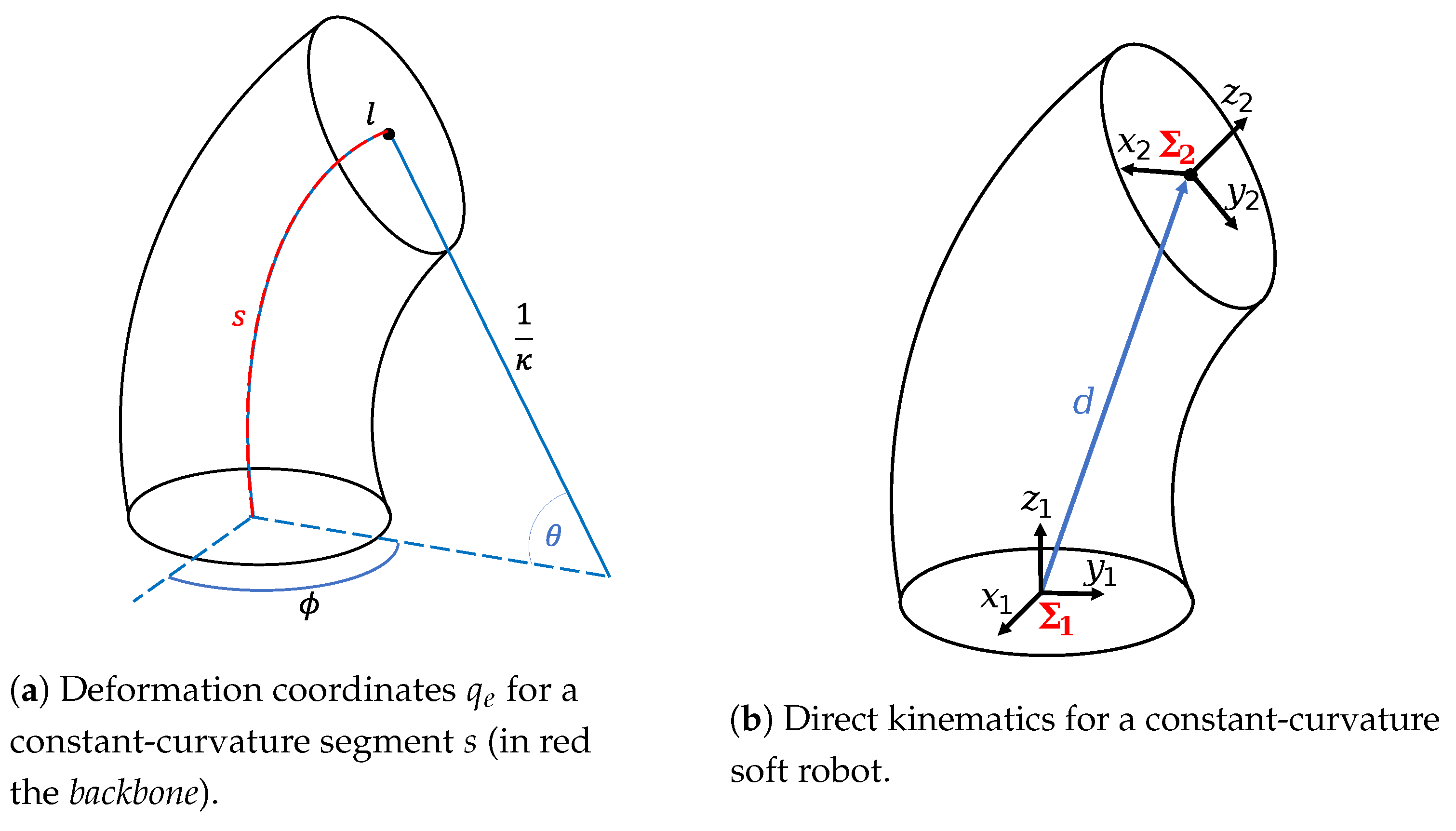
2.1.1. Deformation Coordinates

The proposed soft robot has circumferential and radial restrictions so that it can only have axial and bending deformations, i.e., increasing (or decreasing) its length l and performing flexion in the direction of an azimuth angle $\varphi$ (notice that this is achieved when two or more internal chambers are activated). Given these constraints, we consider constant cross-sectional geometry, which gives rise to defining a curved central axis that passes through the body’s geometric center, known as the backbone (see Figure 2a) [24]. By definition, soft robots have variable curvature along the backbone, i.e., for each cross section of the body, there exists a different curvature. To generate low-cost computation modeling, a constant-curvature approach is used, assuming a single s-curve parameterized by an arc (see Figure 2a), which resembles the body as a segment, hence giving a single curvature $\kappa$ along the segment, which may vary along time. Therefore, a vector of deformation coordinates $q_e$ is defined as

$$q_e={\left(l\varphi \kappa \right)}^T.$$

(1)

The constant curvature parameterizes the backbone of a soft robot by a radius of curvature $r_k={\displaystyle \frac{1}{\kappa }}$ and a curvature angle $\theta =\kappa l$. On the other hand, the constant-curvature approach has the advantage of enabling an additional space named Actuation space ($\mathcal{AS}$), defined by the l vector which contains all length variables $l_1,l_2,...,l_n$ corresponding to the n-actuation elements of the robot. Hence, two direct kinematic mappings arise:

• From actuation space l to configuration space $q_e$ ($\mathcal{AS}\to \mathcal{CS}$), related to the actuation mechanism, which in this case is the length of chambers. It is also known as specific mapping.
• From configuration space $q_e$ to operational space x ($\mathcal{CS}\to \mathcal{OS}$), better known as direct kinematics [25].

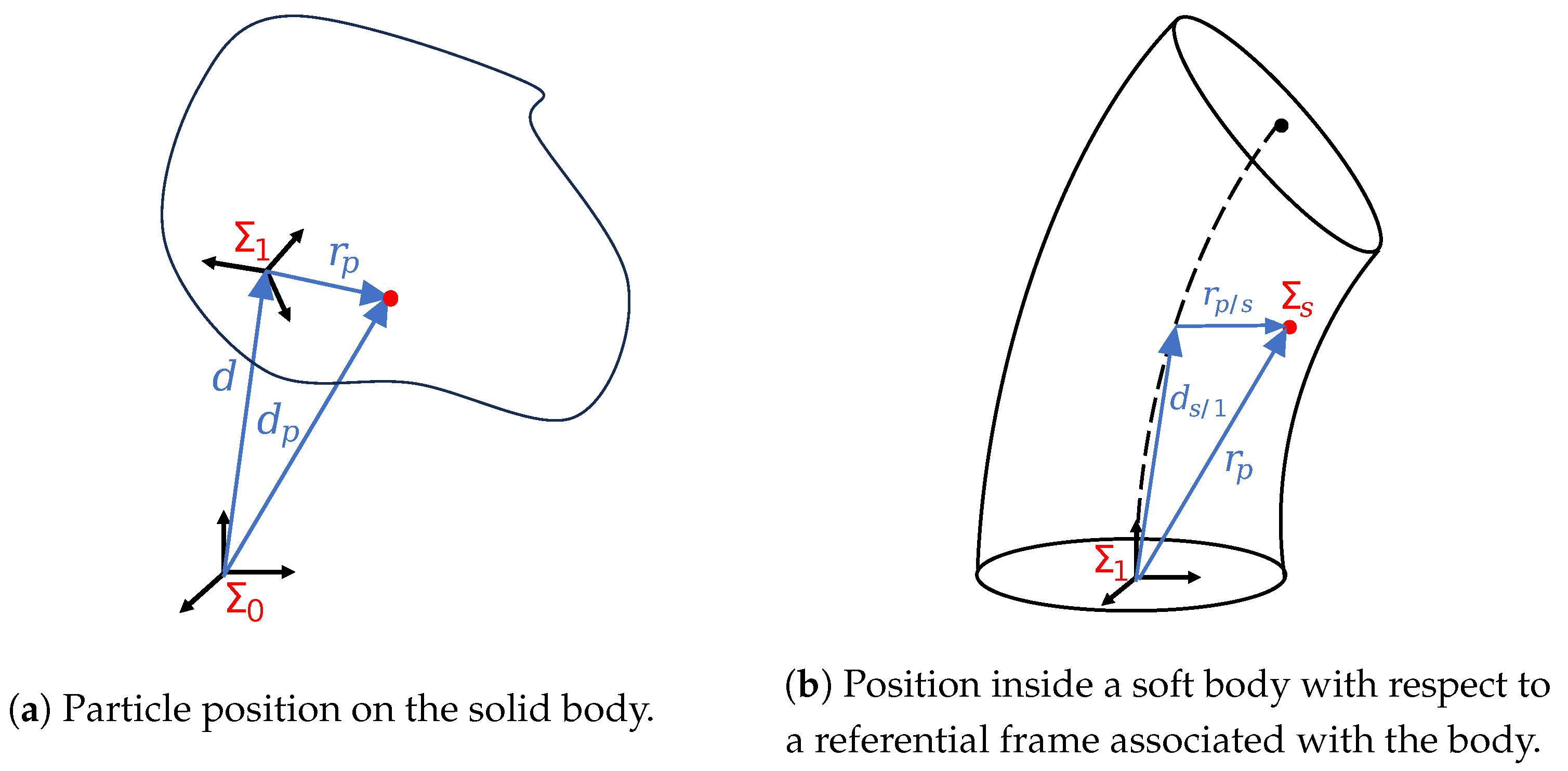
2.1.2. Kinematics

Two frames can describe zeroth-order direct kinematics of a constant-curvature soft robot: the inertial one ${\mathsf{\Sigma }}_1$ at the base of the backbone and the distal reference ${\mathsf{\Sigma }}_2$ at end-effector’s frame, which can be seen in Figure 2b. Consider deformation coordinates $q_e$ and the following homogeneous transformations:

$$\begin{array}{cc}\hfill T\left(q_e\right)& =\left[\begin{array}{cc}{R}_{z,\varphi }& 0_{3\times 1}\\ 0_{1\times 3}& 1\end{array}\right]\left[\begin{array}{cc}{R}_{y,\kappa l}& e\\ 0_{1\times 3}& 1\end{array}\right]\left[\begin{array}{cc}{R}_{z,-\varphi }& 0_{3\times 1}\\ 0_{1\times 3}& 1\end{array}\right]\hfill \\ \hfill & =\left[\begin{array}{cccc}{S}_{\varphi }^2+C_{\varphi }^2{C}_{\kappa l}& -C_{\varphi }{S}_{\varphi }{V}_{\kappa l}& S_{\kappa l}{C}_{\varphi }& C_{\varphi }{\displaystyle \frac{V_{\kappa l}}{\kappa }}\\ -C_{\varphi }{S}_{\varphi }{V}_{\kappa l}& C_{\varphi }^2+S_{\varphi }^2{C}_{\kappa l}& S_{\kappa l}{S}_{\varphi }& S_{\varphi }{\displaystyle \frac{V_{\kappa l}}{\kappa }}\\ -S_{\kappa l}{C}_{\varphi }& -S_{\kappa l}{S}_{\varphi }& C_{\kappa l}& {\displaystyle \frac{S_{\kappa l}}{\kappa }}\\ 0& 0& 0& 1\end{array}\right],\hfill \end{array}$$

(2)

where e is the distal position point obtained by $e={\left(r_k(1-cos\theta )0r_{k}sen\theta \right)}^T$ and $C_x=cos\left(x\right)$, $S_x=sin\left(x\right)$, $V_x=1-cos\left(x\right)$. Let Cartesian position $d_p^{\left(0\right)}$ of a particle p be within the soft body with respect to an inertial reference frame ${\mathsf{\Sigma }}_0$ as an analog to movement transformation of a rigid body, i.e.,

$$d_p^{\left(0\right)}=d+R_0^1\left(\theta \right)r_p^{\left(1\right)},$$

(3)

where d is the body’s position, and $r_p$ is the relative position of point p with respect to local reference frame ${\mathsf{\Sigma }}_1$; see Figure 3 (for the sake of simplicity, Equation (3) is going to be used without superscripts, i.e., $d_p=d+R{r}_p$).

Particle’s velocity ${\dot{d}}_p$ is easily obtained by the time derivative of its position, Equation (3), resulting in

$${\dot{d}}_p=\dot{d}+\dot{R}{r}_p+R{\dot{r}}_p.$$

(4)

It is important to remark that for rigid bodies $R{\dot{r}}_p=0$, the particles position with respect to the inertial reference frame ${\mathsf{\Sigma }}_1$ stays constant during transformation. However, this does not occur for soft robots because the distance between particles is variable due to elastic deformation of the body such that $R{\dot{r}}_p\ne 0$. Additionally, $\dot{R}$ can be expressed in terms of angular velocity $\omega$, using equivalence $\dot{R}=[{\omega }^{\left(0\right)}\times ]R=R[{\omega }^{\left(1\right)}\times ]$, so that a particle’s velocity in a soft body is declared as:

$${\dot{d}}_p=\dot{d}+{\omega }^{\left(0\right)}\times r_p^{\left(0\right)}+R{\dot{r}}_p$$

(5)

and

$$v_p=v+\omega \times r_p+{\dot{r}}_p,$$

(6)

in inertial and local coordinates, respectively. Now, vector $r_p$ can be calculated as a function of deformation coordinates $q_e$ expressed in toroidal coordinates system $c={\left(r\psi \mu \right)}^T$, where r and $\psi$ are the radius and angle which allow it to be positioned in any point of a cross-sectional area within the soft robot; and $\mu \in \left[01\right]$ is the variable which parameterizes an arc length segment (note that $\mu =1$ is the distal point). Therefore, $r_p$ is composed by

$$r_p(q_e,c)=d_{s/1}(q_e,\mu )+R_1^s(q_e,\mu )\left(\begin{array}{c}r{C}_{\psi }\\ r{S}_{\psi }\\ 0\end{array}\right).$$

(7)

where $d_{s/1}$ gives the spatial position of a point s in the backbone, and $r_{p/s}$ positions any point along the s-cross section.

From (7), the relative velocity ${\dot{r}}_p$ of a particle can be obtained by taking its partial derivative with respect to $q_e$:

$${\dot{r}}_p(q_e,{\dot{q}}_e,c)={\displaystyle \frac{\partial r_p(q_e,c)}{\partial q_e}}{\dot{q}}_e=J_{v_p}{\dot{q}}_e.$$

(8)

where $J_{v_p}$ is the deformation Jacobian given by

$$J_{v_p}=\left[\begin{array}{ccc}\mu ·sin\left(\kappa \mu l\right)cos\left(\varphi \right)(1-\kappa r·cos(\varphi -\psi \left)\right)& \frac{\left(cos\right(\kappa \mu l)-1)\left(sin\right(\varphi )-\kappa r·sin(2\varphi -\psi \left)\right)}{\kappa }& -cos\left(\varphi \right)a_1\\ \mu ·sin\left(\kappa \mu l\right)sin\left(\varphi \right)(1-\kappa r·cos(\varphi -\psi \left)\right)& -\frac{\left(cos\right(\kappa \mu l)-1)\left(cos\right(\varphi )-\kappa r·sin(2\varphi -\psi \left)\right)}{\kappa }& -sin\left(\varphi \right)a_1\\ \mu ·cos\left(\kappa \mu l\right)(1-\kappa r·cos(\varphi -\psi \left)\right)& r·sin(\varphi -\psi )sin\left(\kappa \mu l\right)& a_2\end{array}\right],$$

(9)

with $a_1=\frac{{\kappa }^2\mu lr{S}_{\kappa \mu l}{C}_{\varphi }{C}_{\psi }-\kappa \mu l{S}_{\kappa \mu l}-C_{\kappa \mu l}+{\kappa }^2\mu lr{S}_{\kappa \mu l}{S}_{\varphi }{S}_{\psi }+1}{{\kappa }^2}$, and $a_2=-\frac{S_{\kappa \mu l}-\kappa \mu l{C}_{\kappa \mu l}+{\kappa }^2\mu lr{C}_{\varphi -\psi }{C}_{\kappa \mu l}}{{\kappa }^2}$.

2.1.3. Dynamics

Consider the integral Lagrangian model based on the D’Alembert–Lagrange equation to describes deformation of a cylindrical-shaped pneumatic soft robot of constant-curvature in an inertial base [9]:

$$H\left(q\right)\ddot{q}+C(q,\dot{q})\dot{q}+g\left(q\right)-{\tau }_v=\tau ,$$

(10)

with $q={\left(\begin{array}{ccc}l& \varphi & \kappa \end{array}\right)}^T\in {\mathbb{R}}^3$ being the three-dimension vector of generalized coordinates, $H\left(q\right)\in {\mathbb{R}}^{3\times 3}$ the inertia matrix, $C(q,\dot{q})\in {\mathbb{R}}^{3\times 3}$ Coriolis matrix, $g\left(q\right)\in {\mathbb{R}}^3$ the gravity vector, and ${\tau }_v\in {\mathbb{R}}^3$ the generalized viscoelastic force vector which is assumed to be separated and oversimplified in a pure linear viscous friction term and an elastic restorative one of the form ${\tau }_v=-D_v\dot{q}+{\tau }_e$ with positive semi-definite viscous matrix gain $D_v={(d_{q_1},d_{q_2},d_{q_3})}^T$ and generalized elastic forces ${\tau }_e$. The Lagrangian dynamic model (10) has the following properties [9]:

• Symmetry and definite positiveness of inertia matrix: $H\left(q\right)=H^T\left(q\right),H\left(q\right)>0,\forall q$.
• Skew symmetry of Coriolis matrix: $C(·)+C{(·)}^T=\dot{H}\left(q\right)$.
• Passivity: ${\int }_{t_0}^{t_f}\tau ·\dot{q}dt=E\left(t_f\right)-E\left(t_0\right)\ge -E\left(t_0\right)$, for any $E\left(t_0\right)$.

Elastic forces ${\tau }_e$ are obtained via elastic function $U_e\left(q\right)=\frac{1}{2}\frac{AE}{l_0}{\left(l-l_0\right)}^2+\frac{1}{2}\frac{IE}{l_0}{\left(\frac{\kappa l}{2}-{\beta }_0\right)}^2$ proposed in [26] and Castigliano’s theorem [27], as

$${\tau }_e=\frac{\partial U_e}{\partial q}=\left(\begin{array}{c}{\displaystyle \frac{AE}{l_0}}(l-l_0)+{\displaystyle \frac{IE}{l_0}}{\displaystyle \frac{\kappa }{2}}\left({\displaystyle \frac{\kappa l}{2}}-{\beta }_0\right)\\ 0.\\ {\displaystyle \frac{IE}{l_0}}{\displaystyle \frac{l}{2}}\left({\displaystyle \frac{\kappa l}{2}}-{\beta }_0\right)\end{array}\right).$$

2.1.4. Affine Actuation

By considering a pneumatic soft robot with c embedded cylindrical-shaped pneumatic chambers, air injection produces a controlled force field $p={(p_1{p}_2...p_c)}^T\in {\mathbb{R}}^c$ which causes coupled deformation among all chambers inside the body. Thus, a mapping from c pressure vectors to the n generalized force coordinates can be defined as

$$\tau =B\left(q\right)p,$$

(11)

where $B\left(q\right)\in {\mathbb{R}}^{n\times c}$ is the input matrix as a lineal operator given by [9]:

$$\begin{array}{cc}\hfill B\left(q\right)={\displaystyle \frac{\partial }{\partial p}}\left\{{\displaystyle \frac{\partial U_p}{\partial q}}\right\}& =\left[\begin{array}{ccc}\dots & {\displaystyle \frac{\partial V_i\left(q\right)}{\partial q}}& \dots \end{array}\right]\in {\mathbb{R}}^{n\times c}\hfill \end{array}$$

(12)

In this work, a three-DoF soft robot is considered, with three identical prismatic-shaped chambers with transverse area $A_c$ evenly positioned such that all centroids of the chambers’ area are placed along the circumference described by a radius $r_m$, see Figure 4b. Thus, the input matrix $B(·)\in {\mathbb{R}}^{3\times 3}$ is full rank and is rewritten as [12]

$$B\left(q\right)=A_c\left[\begin{array}{ccc}1-\kappa r_{m}cos(-\varphi )& 1-\kappa r_{m}cos\left(\frac{2\pi }{3}-\varphi \right)& 1-\kappa r_{m}cos\left(-\frac{2\pi }{3}-\varphi \right)\\ -\kappa l{r}_{m}sin(-\varphi )& -\kappa l{r}_{m}sin\left(\frac{2\pi }{3}-\varphi \right)& -\kappa l{r}_{m}sin\left(-\frac{2\pi }{3}-\varphi \right)\\ -l{r}_{m}cos(-\varphi )& -l{r}_{m}cos\left(\frac{2\pi }{3}-\varphi \right)& -l{r}_{m}cos\left(-\frac{2\pi }{3}-\varphi \right)\end{array}\right],$$

(13)

where $A_c(r_{ex},w)=\frac{\pi }{3}{(r_{ex}-w)}^2,r_m(r_{ex},w)=\frac{2}{\pi }(r_{ex}-w)sin\left(\frac{\pi }{3}\right).$

2.2. Open-Loop Error Equation

Adding and subtracting the functional

$$\begin{array}{c}\hfill Y_r=H\left(q\right){\ddot{q}}_r+C(q,\dot{q}){\dot{q}}_r+D_v{\dot{q}}_r+g\left(q\right)\end{array}$$

(14)

to (10), we have the open-loop error equation

$$\begin{array}{c}\hfill H\left(q\right){\dot{S}}_r+C(q,\dot{q})S_r+D_v{S}_r=\tau +{\tau }_e-Y_r,\end{array}$$

(15)

where the extended velocity error coordinate is

$$\begin{array}{c}\hfill S_r=\dot{q}-{\dot{q}}_r\end{array}$$

(16)

for ${\dot{q}}_r$, the continuous nominal reference to be defined. System (15) has mainly been used for control design for many Lagrangian systems, even in neuro-control applications. In the latter case, [28] proposes an adaptive neurocontroller with an underlying integral sliding mode to enforce robust error tracking, which does not require training nor any knowledge of the robot with a smooth control actions.

2.2.1. Nominal Reference Design to Induce Integral Sliding Modes

Let the nominal reference be defined as

$$\begin{array}{c}\hfill {\dot{q}}_r={\dot{q}}_d-\alpha \Delta q+S_d-K_i\int \mathrm{sgn}\left(S_q\right),\end{array}$$

(17)

where $\Delta q=q-q_d$ is the position error; $q_d$ and ${\dot{q}}_d$ are the desired position and velocity, respectively; and $\alpha$ and $K_i$ are positive feedback gains, $S_q=S-S_d$, with $S=\Delta \dot{q}+\alpha \Delta q$, $S_d=S\left(t_0\right)e^{-\kappa t}$. Substituting (17) into (16), an extended velocity error coordinates is obtained as

$$\begin{array}{c}\hfill S_r=S_q+K_i\int \mathrm{sgn}\left(S_q\right).\end{array}$$

(18)

2.2.2. Control Design

Based on the seminal work of [13] for rigid robots and extended for soft robot (10) in [9], now, in this paper, given the non-intuitive free-form deformation of the continuum soft robot, we wonder how to consider the body deformation in the control design to guarantee $S\to 0$ with performance evaluation. More precisely, we are interested in designing $\tau$ for unknown (10), considering how deformation coordinates perform, additionally to guarantee tracking error convergence.

2.3. Problem Statement

We are interested in how to control soft robots using reinforcement learning tools, explicitly using the Actor–Critic scheme. Necessarily, it implies introducing an additional metric for task-performance evaluation along with error convergence. Thus, the following problem arises:

“Design a learning mechanism that guarantees simultaneous error convergence and task performance of a closed-loop pneumatic-driven soft robot through a control law that evaluates online learning units for a model-free scheme.”

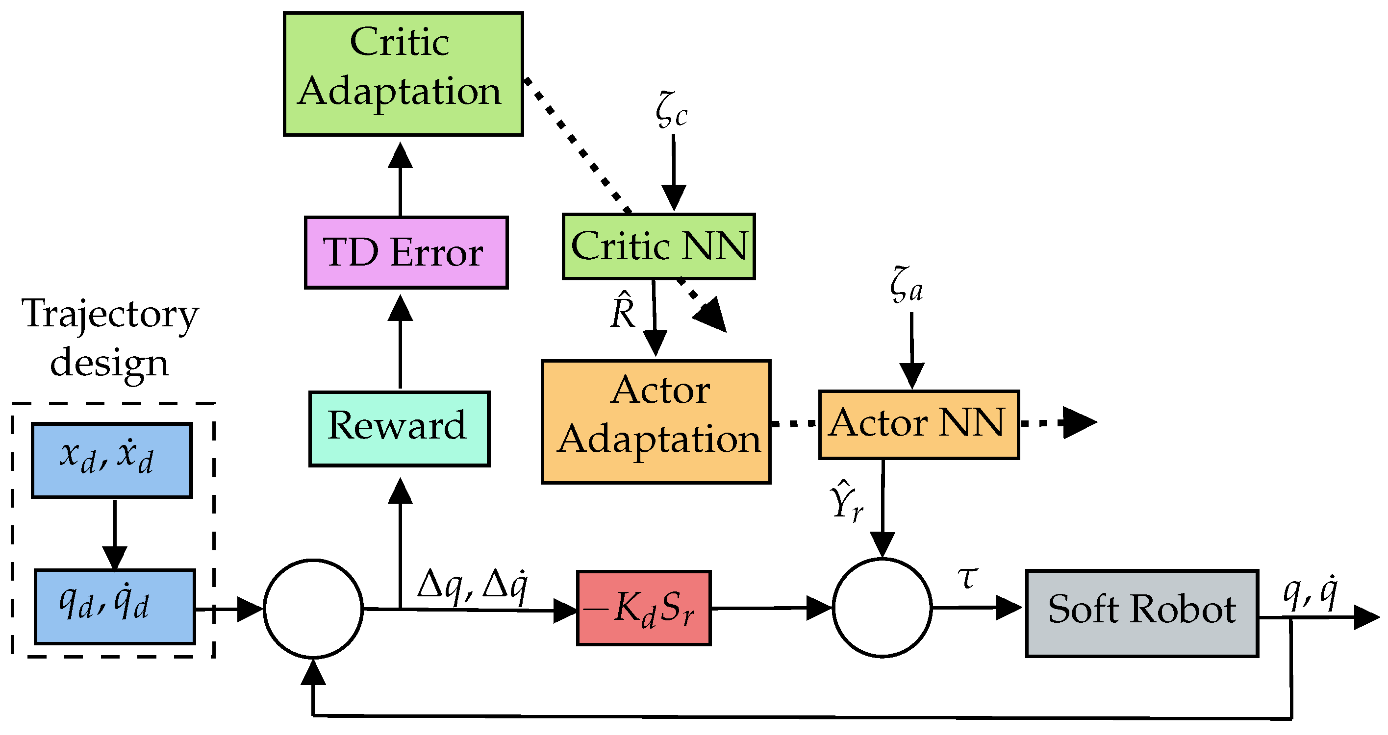
3. Actor–Critic Learning of Motor Control

Now, we proceed to explain in detail the proposed Actor–Critic architecture as well as the main result called Reinforced Neurocontroller; see Figure 5.

3.1. Reward-Based Value Function and Temporal Difference Error

Consider the following continuous value function R that depends only on the task-dependent scalar reward $r\in \mathbb{R}$ [29];

$$R={\int }_{t_0}^{\infty }{e}^{-\frac{m-t}{\psi }}r\left(m\right)dm,$$

(19)

where $\psi$ is the time constant for discounting future rewards with $t\le m\le \infty$. Differentiating (19), one obtains

$$\dot{R}=\frac{1}{\psi }R-r\left(t\right),$$

(20)

which can be rewritten in terms of an error $\delta$, as the so-called temporal difference error for continuous time [29],

$$\delta =\dot{R}-\frac{1}{\psi }R+r.$$

(21)

This consistency equation is used to approximate value function (19) based only on reward information.

Remark 1. 

Notice that in the proposed Actor–Critic scheme, the reward and the temporal difference error implement the learning mechanism in the Critic NN that approximates the value function $\widehat{R}$, which in turn represents the reinforcement signal used to improve the adaptation mechanism of the Actor NN that approximates $Y_r$ by ${\widehat{Y}}_r$.

3.2. Critic NN

Given that value function from Equation (19) is smooth, it can be approximated by a neural network with finite constant weights $W_c\in {\mathbb{R}}^c$ and input basis $Z_c(·)\in {\mathbb{R}}^c$ such that

$$\begin{array}{c}\hfill R=W_c^T{Z}_c(·)+{ϵ}_c,\end{array}$$

(22)

where a small ${ϵ}_c$ is the neural approximation error. Then, there exists a neural network with adaptive weights ${\widehat{W}}_c\in {\mathbb{R}}^c$ that approximates (22) as follows

$$\begin{array}{cc}\hfill \widehat{R}& ={\widehat{W}}_c^T{Z}_c(·)\hfill \end{array}$$

(23)

where $Z_c(·)=\sigma \left(V_c^T{\zeta }_c\right)\in {\mathbb{R}}^c$ is the sigmoid bipolar activation function, with $V_c\in {\mathbb{R}}^{3\times c}$ representing fixed weights and ${\zeta }_c\in {\mathbb{R}}^c$ being the input vector. It means that the learning has been made. Now, using (23) instead of (22) by the equivalence principle, the temporal difference error (21) can be written as

$$\begin{array}{cc}\hfill \widehat{\delta }=& \dot{\widehat{R}}-\frac{1}{\psi }\widehat{R}+r\hfill \\ \hfill =& {\dot{\widehat{W}}}_c^T\sigma (·)+{\widehat{W}}_c^T{\dot{\sigma }}_c(·)-\frac{1}{\psi }{\widehat{W}}_c^T{\sigma }_c(·)+r.\hfill \end{array}$$

(24)

Notice that $\widehat{\delta }\ne 0$ per se (it is in the neural error domain); thus, the problem becomes in designing the adaptation ${\dot{\widehat{W}}}_c$ such that $\widehat{\delta }\to 0$, which translates into an appropriate approximation of (19) by (23). Now, we have the following result.

Proposition 1. 

Consider the following adaptation law

$$\begin{array}{cc}\hfill {\dot{\widehat{W}}}_c& =-K_{w}sgn\left({\widehat{W}}_c\right)-Ksgn\left(\widehat{\gamma }\right)\frac{{\sigma }_c(·)}{{\sigma }_c^T(·){\sigma }_c(·)},\hfill \end{array}$$

(25)

and

$$\widehat{\gamma }=\widehat{R}-\frac{1}{\psi }{\int }_{t_0}^{t_f}R+{\int }_{t_0}^{t_f}r,$$

(26)

which comes from the temporal difference error $\widehat{\delta }$. Then, selecting $K_w$ and K large enough, the convergence of the temporal difference error is achieved such that $\widehat{\delta }\to 0$.

Proof. 

See Appendix A.1.  □

3.3. Actor NN

Let (14), according to the NN approximation property, be the continuous nonlinear function; it can be represented as $Y_r=W_a^T{Z}_a(·)+{ϵ}_a$, with $W_a\in {\mathbb{R}}^{a\times 3}$ finite constant weights, $Z_a(·)\in {\mathbb{R}}^a$ being the input basis, and ${ϵ}_a$ being the reconstruction error. Then, the following neural network and adaptation law are proposed

$$\begin{array}{cc}\hfill {\widehat{Y}}_r& ={\widehat{W}}_a^T{Z}_a(·),\hfill \end{array}$$

(27)

$$\begin{array}{cc}\hfill {\dot{\widehat{W}}}_a& =-{\mathsf{\Gamma }}_a{\sigma }_a^T(·)S_r^T-{\mathsf{\Gamma }}_a{\widehat{W}}_a{\left(\widehat{\gamma }r\right)}^2,\hfill \end{array}$$

(28)

where ${\widehat{W}}_a\in {\mathbb{R}}^{a\times 3}$ is the matrix of adaptive weights, $Z_a(·)={\sigma }_a\left(V_a^T{\zeta }_a\right)\in {\mathbb{R}}^a$ is the bipolar sigmoid activation function, with $V_a\in {\mathbb{R}}^{4\times a}$ being the matrix of fixed weights and ${\zeta }_a\in {\mathbb{R}}^4$ the input vector, and ${\mathsf{\Gamma }}_a\in {\mathbb{R}}^{a\times a}$ is positive definite gain.

3.4. Passivity-Based Reinforced Neurocontroller

Let the control signal be defined as

$$\begin{array}{c}\hfill \tau =-K_d{S}_r+{\widehat{Y}}_r,\end{array}$$

(29)

with $K_d>0\in {\mathbb{R}}^{3\times 3}$. Then, the following main results are in order.

Theorem 1. 

Consider the soft robot dynamics (10) in a closed-loop with the control signal (29) and adaptation laws (25) and (28). Thus, from Proposition 1, for high enough $K_i$ and $K_d$ gains, exponential convergence of the tracking errors is guaranteed via integral sliding modes with smooth control signals and without knowledge of the soft robot dynamics.

Proof. 

See Appendix A.2.  □

4. Numerical Simulations

4.1. The Simulator and Parameters

The soft robot aims to track a tornado-like trajectory at a distal point described by a desired pose $X_d$; see Figure 6. Notice that $X_d$ was mapped into generalized coordinates $q_d$ via first-order inverse kinematics. Simulations were carried out in Matlab-Simulink 2021b with solver ode23tb running at an adaptive step sampling for a tolerance of $1\times {10}^{-3}$.

Table 1. Soft robot parameters and the tornado-like desired trajectory.

Variable	Description	Value
$r_{ex}$	External radius	$0.1$ m
w	Wall width	$0.001$ m
$l_0$	Initial length	$0.9$ m
${\beta }_0$	Initial bending	$0.6285$ rad
E	Young’s modulus	$0.15$ MPa
$X_d=\left[\begin{array}{c}{x}_d\\ y_d\\ z_d\end{array}\right]$	Desired pose	$\left[\begin{array}{c}0.7sin(t/50)+0.01tsin\left(t\right)+0.2\\ 0.7cos(t/50)+0.01tcos\left(t\right)-0.5\\ 0.1+0.01t\end{array}\right]$

shows the dynamic parameters and desired trajectory of the soft robot, with the Young’s modulus value being based on experiments [30] using Ecoflex 00–30™. Initial bending ${\beta }_0$ was calculated through initial length and curvature as ${\beta }_0={\displaystyle \frac{l_0\times {\kappa }_0}{2}}$.

4.2. Neural Network Architectures

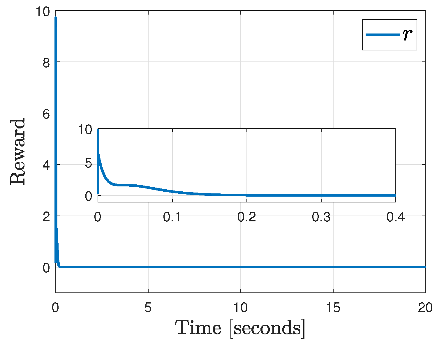
The Critic NN has only one hidden layer, with input vector ${\zeta }_c=(-1\Delta q)$, where weights connect the input layer to the hidden layer with constants $V_c$; initial adaptive weights ${\widehat{W}}_c\left(t_0\right)$ are tuned between 0 and 1. Similarly, the Actor neural network has one hidden layer with input vector ${\zeta }_a=(1\int S_r)$, where the weights connecting the input layer and the hidden layer $V_a$ are fixed.

4.3. Reward Design

Given that the reward function, r, encodes critical aspects to motivate the fulfillment of the task, and the soft robots are typically equipped with low resolution (due to embedded sensor technology being in progress), it is worth considering weight position over velocity errors. Then, let the reward function be

$$\begin{array}{c}\hfill r=\frac{1}{2}\left(\Delta q^{T}P\Delta q+\Delta {\dot{q}}^{T}Q\Delta \dot{q}\right)\end{array}$$

(30)

where $P=diag(9,9,9)$, $Q=diag(1,1,1)$.

4.4. Feedback Control and Adaptation Gains

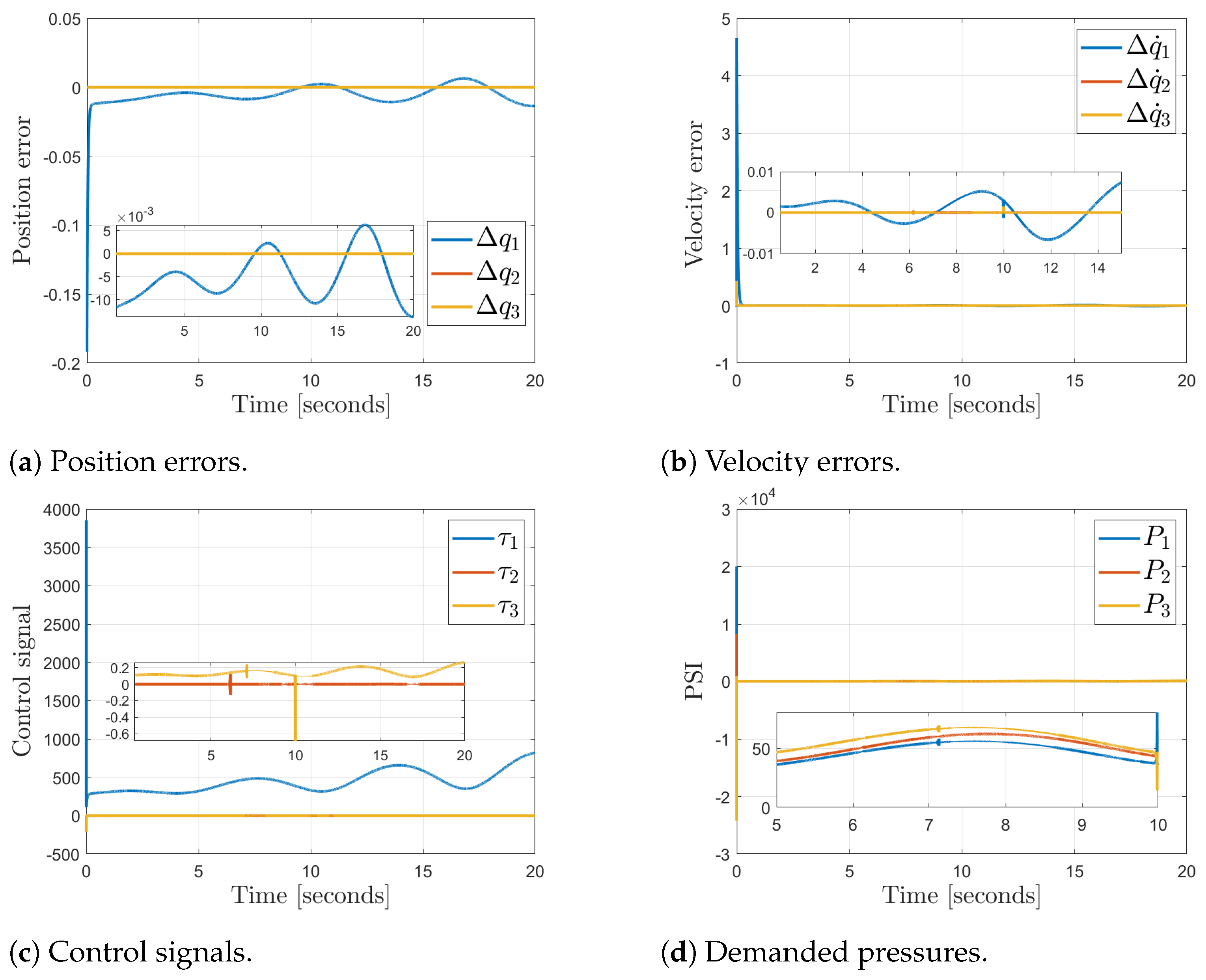
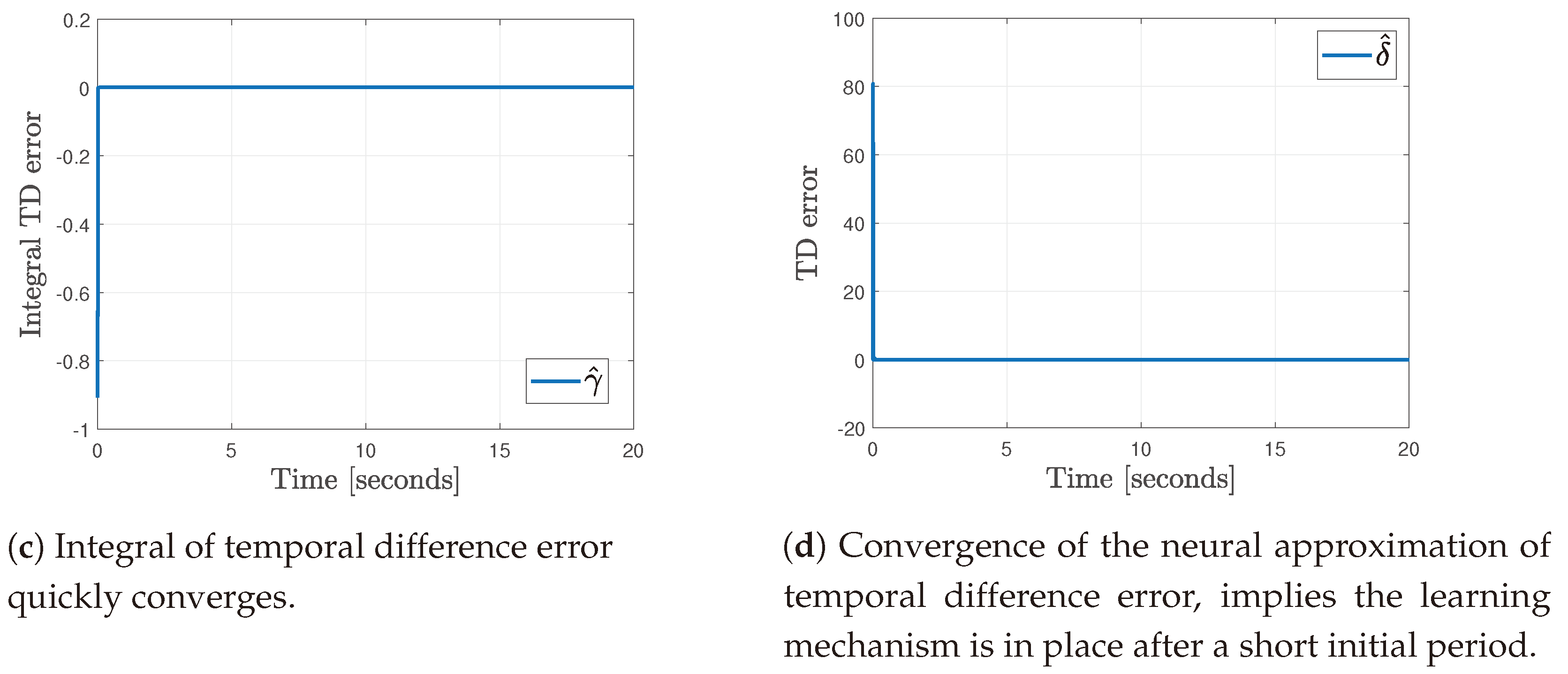
The final value of feedback and adaptation gains follow the simulator’s theory specifications and numerical performance. The values for feedback gains were $K_d=diag\left(1000200200\right)$, $\alpha =diag\left(202020\right)$, $K_i=diag\left(0.050.050.05\right)$, and $\kappa =30$; and for the adaptation gains, they were $K=50$, $K_w=7$, and ${\mathsf{\Gamma }}_a=I_{10\times 10}\times 4000$. It aims to promote larger reward recollection from smaller position errors, so evaluation-based reinforcement is influenced to take action even by smaller position errors.

4.5. Results

From Figure 6, we notice that despite the fact that initial conditions are selected away from the desired trajectory, the end-effector tracks the desired trajectory with a short transient. This can be seen in Figure 7, where tracking error converges exponentially in about $t=0.3$ s. Figure 8a shows the bounded extended velocity error $S_r$ that shapes the invariant of stability, which gives rise to sliding mode at $S_q=0$; see Figure 8b around $t\ge 0.3$ s. The control signals are quite smooth; see Figure Figure 9a. Notice that ${\tau }_1$ corresponds to the length coordinate l where its magnitude is much greater than ${\tau }_2$ and ${\tau }_3$ due to the higher energy that is required to deform the material for elongation tasks. Figure 9c,d shows the integral and temporal difference errors converging quickly, implying an accurate approximation of the value function by the Critic NN. Finally, reward behavior is shown in Figure 10, since it depends on the evaluation of tracking errors (30); since it has a larger value at initial conditions, then at the beginning, it reaches its higher value. Once the end effector reaches the desired trajectory, the reward ceases signaling that motor learning is achieved.

Comparative Results vs. Classical PID Controller

In order to compare how our proposal performs against others, simulations were also carried out for the very well-known controller, such as classical model-free PID regulator, under the same desired trajectories and initial conditions. The results are shown in Figure 11. Generalized position and velocity errors are shown in Figure 11a and Figure 11b, respectively. Notice that trajectories remain bounded after a short initial response. In contrast, our scheme converges to the origin; see Figure 7. Figure 11c,d shows the control signals and the demanded pressures. Notice that for initial time $t<0.1$, the system has a high demand of control effort, translating into a high-pressure demand, which can be detrimental in practice. In contrast, our scheme ameliorates this effect and achieves convergence of tracking errors with smooth control; see Figure 7 and Figure 9a,b.

5. Discussions

5.1. On the Actor–Critic Architecture with Adaptive Neural Weights

The Actor and Critic neural networks interplay to guarantee tracking, taking into consideration the soft robot performance. The Critic NN approximates the value function by enforcing convergence of the integral and the temporal difference error. In contrast, the Actor NN approximates the nonlinear dynamics using online reinforcement from the Critic NN throughout its weights and the reward. Reward design is fundamental to yield information about the robot task performance. Given the subtleties of the soft robot, reward design is based on the weighted sum of the position and velocity tracking errors. However, the reward can be designed otherwise, since its interpretation depends on what promotes learning. Adaptation of Actor–Critic’s weights is proposed based on Lyapunov stability, in contrast to other works that use variants of the gradient descent method.

5.2. On Simulation Study

It is considered to be a Lagrangian soft robot assuming constant cross-section geometry along the backbone, even after being exposed to exogenous and endogenous forces. In practice, this is achieved by manufacturing inextensible threads that braid the soft robot [17] to restrict deformation when pressurized. However, this constraint may not be enforced for negative absolute or relative pressure or when a vacuum emerges. Further research is needed from the material science community to considered these cases.

5.3. Advantages, Disadvantages, and Limitations

The advantages of this method are as follows: the proposed AC scheme is model-free, i.e., no information on the soft robot dynamics is needed to implement the scheme. In addition, neither pre-training nor initialization is required in the learning process. Surprisingly, Actor–Critic neural network topologies are of low dimension for such difficult and complex nonlinear soft robot dynamics, with only one hidden layer of neurons. We address the difficult and complex soft robot continuum dynamics based on density variations that yield a varying center of mass and a varying inertia tensor. On the other hand, as a limitation, the model has a kinematic singularity at $\kappa =0$, which is common with other soft robot models, as well as the assumption of constant cross area, which is hard to enforce in practice. Then, for practical implementations of this RL scheme, we surmise that the challenge also includes the soft robot hardware, actuation, and sensory system.

Other modeling domains, such as FEM, have been used as an alternative to study the approximate mechanical properties of soft robots [31,32], with quite some success in designing and manufacturing deformable bodies. Certainly, FEM is needed to analyze structurally optimal designs and comparisons to its continuum domain.

6. Conclusions

Contributions from many research fields have enriched soft robot knowledge, giving rise to novel paradigms on modeling, control, and design. In this note, a novel RL controller for a class of continuum soft robot model is addressed, contributing to the state-of-the-art in learning how to yield 3D trajectories, taking into account online evaluation of deformation performance. The stability-guaranteed, model-free neurocontroller oversees the convergence of the tracking error and reward recollection while exploiting its structural properties, including passivity. The key contribution comes from novel designs of nonlinear adaptive weights of the Critic NN and Actor NN, the former of which uses discontinuous terms and nonlinear activations functions to enforce convergence of TD errors $\widehat{\delta }$. In contrast, the latter is influenced by the reinforcement signals given by the reward and temporal difference error. The soft robot under consideration is of the class of continuum body deformation driven by internal pneumatic chambers. This soft robot model has a Lagrangian structure; henceforth, our RL scheme is not limited to soft robots, but it can be implemented in systems characterized by Lagrangian dynamics. Real-time experimental testing has major importance in pursuing real compliance with the theory based on the axioms and the assumptions. Ongoing effort is occuring in the development of such a platform with special care on non-invasive measurement system and low-level pneumatic control instrumentation [9].

References

1. Barto, A.G.; Sutton, R.S.; Anderson, C.W. Looking Back on the Actor—Critic Architecture. IEEE Trans. Syst. Man Cybern. Syst. 2021, 51, 40–50. [Google Scholar] [CrossRef]
2. Wang, F.Y.; Zhang, H.; Liu, D. Adaptive Dynamic Programming: An Introduction. IEEE Comput. Intell. Mag. 2009, 4, 39–47. [Google Scholar] [CrossRef]
3. Lewis, F.; Vrabie, D.; Syrmos, V. Optimal Control; EngineeringPro Collection; Wiley: Hoboken, NJ, USA, 2012. [Google Scholar]
4. Guo, K.; Pan, Y. Composite adaptation and learning for robot control: A survey. Annu. Rev. Control. 2023, 55, 279–290. [Google Scholar] [CrossRef]
5. Jin, L.; Li, S.; Yu, J.; He, J. Robot manipulator control using neural networks: A survey. Neurocomputing 2018, 285, 23–34. [Google Scholar] [CrossRef]
6. He, W.; Chen, Y.; Yin, Z. Adaptive Neural Network Control of an Uncertain Robot with Full-State Constraints. IEEE Trans. Cybern. 2016, 46, 620–629. [Google Scholar] [CrossRef] [PubMed]
7. Song, B.; Slotine, J.J.; Pham, Q.C. Stability Guarantees for Continuous RL Control. arXiv 2022, arXiv:cs.RO/2209.07324. [Google Scholar]
8. Bhagat, S.; Banerjee, H.; Ho Tse, Z.T.; Ren, H. Deep reinforcement learning for soft, flexible robots: Brief review with impending challenges. Robotics 2019, 8, 4. [Google Scholar] [CrossRef]
9. Trejo-Ramos, C.A.; Olguín-Díaz, E.; Parra-Vega, V. Lagrangian and Quasi-Lagrangian Models for Noninertial Pneumatic Soft Cylindrical Robots. J. Dyn. Syst. Meas. Control. 2022, 144, 121004. [Google Scholar] [CrossRef]
10. Guan, Z.; Yamamoto, T. Design of a Reinforcement Learning PID controller. In Proceedings of the 2020 International Joint Conference on Neural Networks (IJCNN), Glasgow, UK, 19–24 July 2020; pp. 1–6. [Google Scholar] [CrossRef]
11. He, W.; Gao, H.; Zhou, C.; Yang, C.; Li, Z. Reinforcement Learning Control of a Flexible Two-Link Manipulator: An Experimental Investigation. IEEE Trans. Syst. Man Cybern. Syst. 2021, 51, 7326–7336. [Google Scholar] [CrossRef]
12. Vázquez-García, C.E.; Trejo-Ramos, C.A.; Parra-Vega, V.; Olguín-Díaz, E. Quasi-static Optimal Design of a Pneumatic Soft Robot to Maximize Pressure-to-Force Transference. In Proceedings of the 2021 Latin American Robotics Symposium (LARS), 2021 Brazilian Symposium on Robotics (SBR), and 2021 Workshop on Robotics in Education (WRE), Natal, Brazil, 11–15 October 2021; pp. 126–131. [Google Scholar]
13. Parra-Vega, V.; Arimoto, S.; Liu, Y.H.; Hirzinger, G.; Akella, P. Dynamic sliding PID control for tracking of robot manipulators: Theory and experiments. IEEE Trans. Robot. Autom. 2003, 19, 967–976. [Google Scholar] [CrossRef]
14. Yang, T.; Xiao, Y.; Zhang, Z.; Liang, Y.; Li, G.; Zhang, M.; Li, S.; Wong, T.W.; Wang, Y.; Li, T.; et al. A soft artificial muscle driven robot with reinforcement learning. Sci. Rep. 2018, 8, 14518. [Google Scholar] [CrossRef]
15. Ishige, M.; Umedachi, T.; Taniguchi, T.; Kawahara, Y. Exploring Behaviors of Caterpillar-Like Soft Robots with a Central Pattern Generator-Based Controller and Reinforcement Learning. Soft Robot. 2019, 6, 579–594. [Google Scholar] [CrossRef] [PubMed]
16. Boyraz, P.; Runge, G.; Raatz, A. An overview of novel actuators for soft robotics. Actuators 2018, 7, 48. [Google Scholar] [CrossRef]
17. Cianchetti, M.; Ranzani, T.; Gerboni, G.; De Falco, I.; Laschi, C.; Menciassi, A. STIFF-FLOP surgical manipulator: Mechanical design and experimental characterization of the single module. In Proceedings of the 2013 IEEE/RSJ International Conference on Intelligent Robots And Systems, Tokyo, Japan, 3–7 November 2013; pp. 3576–3581. [Google Scholar]
18. Xu, F.; Wang, H.; Au, K.W.S.; Chen, W.; Miao, Y. Underwater dynamic modeling for a cable-driven soft robot arm. IEEE/ASME Trans. Mechatronics 2018, 23, 2726–2738. [Google Scholar] [CrossRef]
19. Marchese, A.D.; Katzschmann, R.K.; Rus, D. A recipe for soft fluidic elastomer robots. Soft Robot. 2015, 2, 7–25. [Google Scholar] [CrossRef]
20. Marchese, A.D.; Komorowski, K.; Onal, C.D.; Rus, D. Design and control of a soft and continuously deformable 2d robotic manipulation system. In Proceedings of the 2014 IEEE International Conference ON Robotics And Automation (ICRA), Hong Kong, China, 31 May–7 June 2014; pp. 2189–2196. [Google Scholar]
21. Katzschmann, R.K.; Marchese, A.D.; Rus, D. Autonomous object manipulation using a soft planar grasping manipulator. Soft Robot. 2015, 2, 155–164. [Google Scholar] [CrossRef]
22. Connolly, F.; Walsh, C.J.; Bertoldi, K. Automatic design of fiber-reinforced soft actuators for trajectory matching. Proc. Natl. Acad. Sci. USA 2017, 114, 51–56. [Google Scholar] [CrossRef]
23. Hannan, M.W.; Walker, I.D. Kinematics and the implementation of an elephant’s trunk manipulator and other continuum style robots. J. Robot. Syst. 2003, 20, 45–63. [Google Scholar] [CrossRef]
24. Sadati, S.H.; Naghibi, S.E.; Shiva, A.; Noh, Y.; Gupta, A.; Walker, I.D.; Althoefer, K.; Nanayakkara, T. A geometry deformation model for braided continuum manipulators. Front. Robot. AI 2017, 4, 22. [Google Scholar] [CrossRef]
25. Webster, R.J., III; Jones, B.A. Design and kinematic modeling of constant curvature continuum robots: A review. Int. J. Robot. Res. 2010, 29, 1661–1683. [Google Scholar] [CrossRef]
26. Godage, I.S.; Branson, D.T.; Guglielmino, E.; Medrano-Cerda, G.A.; Caldwell, D.G. Shape function-based kinematics and dynamics for variable length continuum robotic arms. In Proceedings of the 2011 IEEE International Conference on Robotics and Automation, Shanghai, China, 3–9 May 2011; pp. 452–457. [Google Scholar]
27. Odom, E.M.; Egelhoff, C.J. Teaching deflection of stepped shafts: Castigliano’s theorem, dummy loads, heaviside step functions and numerical integration. In Proceedings of the 2011 Frontiers in Education Conference (FIE), Rapid City, SD, USA, 12–15 October 2011; pp. F3H-1–F3H-6. [Google Scholar] [CrossRef]
28. Garcia, R.; Parra-Vega, V. Tracking control of robot manipulators using second order neuro sliding mode. Lat. Am. Appl. Res. 2009, 39, 285–294. [Google Scholar]
29. Doya, K. Temporal Difference Learning in Continuous Time and Space. In Advances in Neural Information Processing Systems; Touretzky, D., Mozer, M., Hasselmo, M., Eds.; MIT Press: Cambridge, MA, USA, 1995; Volume 8, pp. 1073–1079. [Google Scholar]
30. Kandasamy, S.; Teo, M.; Ravichandran, N.; McDaid, A.; Jayaraman, K.; Aw, K. Body-powered and portable soft hydraulic actuators as prosthetic hands. Robotics 2022, 11, 71. [Google Scholar] [CrossRef]
31. Bieze, T.M.; Largilliere, F.; Kruszewski, A.; Zhang, Z.; Merzouki, R.; Duriez, C. Finite Element Method-Based Kinematics and Closed-Loop Control of Soft, Continuum Manipulators. Soft Robot. 2018, 5, 348–364. [Google Scholar] [CrossRef] [PubMed]
32. Sun, Y.; Zhang, D.; Liu, Y.; Lueth, T.C. FEM-Based Mechanics Modeling of Bio-Inspired Compliant Mechanisms for Medical Applications. IEEE Trans. Med. Robot. Bionics 2020, 2, 364–373. [Google Scholar] [CrossRef]
Figure 1. Characteristic deformations of a cylindrical-shaped soft robot.
Robotics 12 00141 g001
Figure 2. Deformation coordinates with respect to referential frames Σ 1 , Σ 2 .
Robotics 12 00141 g002
Figure 3. Position of a particle in a continuum soft body.
Robotics 12 00141 g003
Figure 4. Soft robot proposed geometry.
Robotics 12 00141 g004
Figure 5. The proposed Actor–Critic scheme where each colored block corresponds to a specific role in the scheme. Notice that it keeps the conventional neurocontroller architecture approximating Y ^ r .
Robotics 12 00141 g005
Figure 6. Tracking of 3D soft robot desired (red dotted line) trajectories X d ( t ) , from initial pose (green dot) shown in grey with a black backbone to a final pose shown in orange, with red backbone.
Robotics 12 00141 g006
Figure 7. Position and velocity tracking errors exhibit smooth convergence, with a short transient of about 300 ms. Notice that such a performance for such aggressive trajectories, since Coriolis (centrifugal and centripetal) forces increases as time goes by.
Robotics 12 00141 g007
Figure 8. Performance of extended velocity error S r and invariant manifolds S q = 0 suffers from the increment of Coriolis forces; nonetheless, sliding modes are enforced.
Robotics 12 00141 g008
Figure 9. (a) Control signals and (b) pressure behavior, in accordance to the convergence of (c) integral temporal difference error and (d) temporal difference error.
Robotics 12 00141 g009aRobotics 12 00141 g009b
Figure 10. Surprisingly, reward converges after a very short transient.
Robotics 12 00141 g010
Figure 11. [Classical PID controller]. Results obtained using PID: (a) position errors remains bounded, similarly, (b) the velocity errors also remain bounded. (c) control signals exhibit high demand and produces pressures (d).
Robotics 12 00141 g011