Article

Length Modelling of Spiral Superficial Soft Strain Sensors Using Geodesics and Covering Spaces

1
Australian Centre for Field Robotics (ACFR), The University of Sydney, Sydney, NSW 2006, Australia
2
e:fs Techhub GmbH, 85080 Gaimersheim, Germany
3
Shenzhen Key Laboratory of Control Theory and Intelligent Systems, and the Guangdong Provincial Key Laboratory of Human-Augmentation and Rehabilitation Robotics in Universities, Southern University of Science and Technology, Shenzhen 518055, China
*
Author to whom correspondence should be addressed.
Robotics 2023, 12(6), 164; https://doi.org/10.3390/robotics12060164
Submission received: 14 October 2023 / Revised: 22 November 2023 / Accepted: 23 November 2023 / Published: 1 December 2023
(This article belongs to the Special Issue Editorial Board Members' Collection Series: "Soft Robotics")

Abstract

:
Piecewise constant curvature soft actuators can generate various types of movements. These actuators can undergo extension, bending, rotation, twist, or a combination of these. Proprioceptive sensing provides the ability to track their movement or estimate their state in 3D space. Several proprioceptive sensing solutions were developed using soft strain sensors. However, current mathematical models are only capable of modelling the length of the soft sensors when they are attached to actuators subjected to extension, bending, and rotation movements. Furthermore, these models are limited to modelling straight sensors and incapable of modelling spiral sensors. In this study, for both the spiral and straight sensors, we utilise concepts in geodesics and covering spaces to present a mathematical length model that includes twist. This study is limited to the Piecewise constant curvature actuators and demonstrates, among other things, the advantages of our model and the accuracy when including and excluding twist. We verify the model by comparing the results to a finite element analysis. This analysis involves multiple simulation scenarios designed specifically for the verification process. Finally, we validate the theoretical results with previously published experimental results. Then, we discuss the limitations and possible applications of our model using examples from the literature.

1. Introduction

Soft pneumatic actuators (SPAs) are known for their flexibility and their ability to undergo large deformations. They can be designed to mimic natural and biological organs as well as provide safe interaction with people [1]. These actuators, however, fall behind their rigid counterparts in the ability to sense their state in planar or 3D spaces. Soft actuators can have infinite degrees of freedom (DOFs) and can be deformed by both internal and external loads. Predicting the response of these soft actuators accurately via modelling alone is difficult due to their complex behaviours induced by non-linearity and viscoelastic effects, and hence state sensing and estimation are required [2].
State sensing can be achieved by using external monitoring such as motion capture cameras [3] or electromagnetic tracking [4]. However, these techniques are designed to work within a lab environment. Alternatively, proprioceptive sensing [5] can sense the actuator state inside or outside the lab environment. Several proprioceptive techniques were developed [6] that utilise superficial soft strain sensors which measure the local change in the length between two points on the surface. The mathematical models that represent the length of these sensors depend on their position as well as the soft actuator model, movement, and reinforcement. The model accuracy can be verified via simulation, with finite element analysis (FEA) for example, and/or validated via experiments [7].

1.1. Common Soft Actuator Models

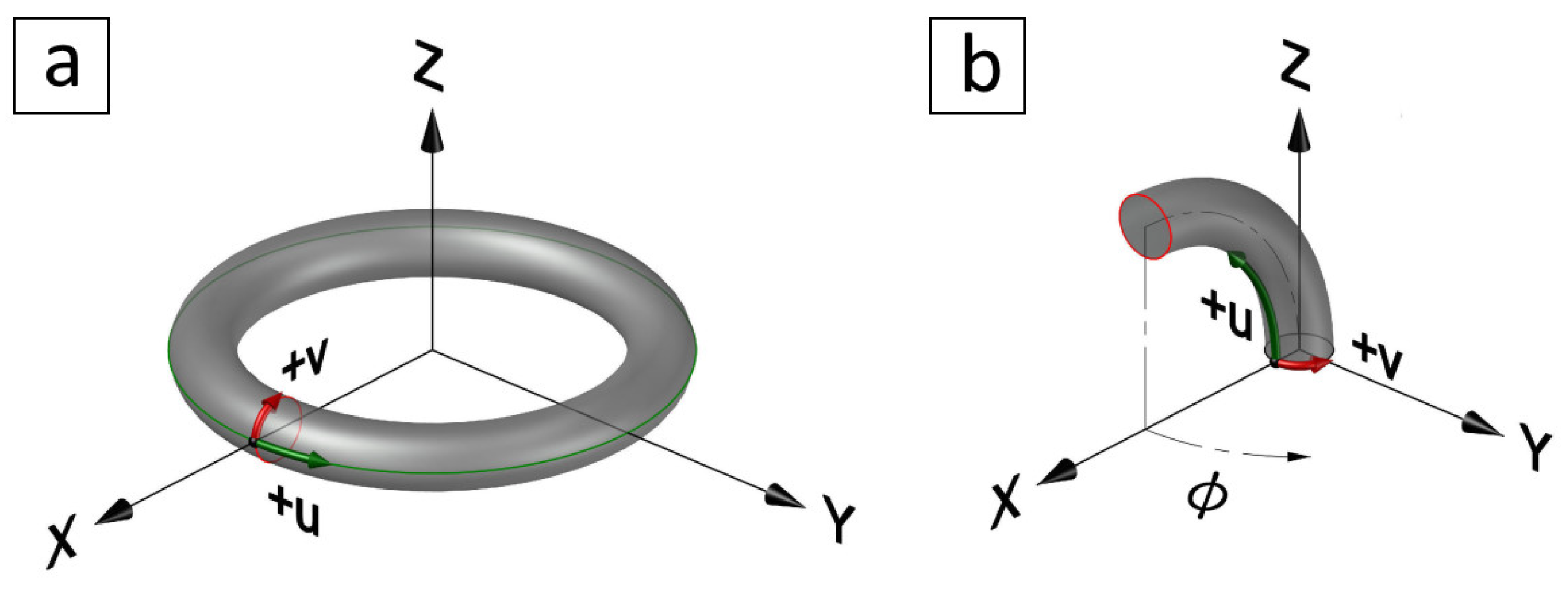
Soft actuators are generally modelled as curves with either a variable curvature or a piecewise constant curvature (PCC) approach, Figure 1a,b. For variable curvatures[8], the actuator can be considered as a slender rod and modelled via the Cosserat rod model (CRM). While for PCCs, the actuator can be modelled via several methods [9]. Additionally, a hybrid approach known as piecewise constant strain (PCS) [10] is used to model soft actuators. The PCS model extends the constant curvature assumption to more general rod kinematics and provides a simpler dynamic model than CRM. As shown in Figure 1c, the soft actuator basic movements can be categorised as extension, bending/rotation, twist, and shear [8]. The twist is a mechanical rotation about a certain point or axis caused by a torque acting on that point or axis. However, some textbooks may define the term "twist", denoted by V , as the time derivative of the actuator end point pose [11]. The PCC model can only represent extension, bending, and rotation movements. Both CRM and PCS can represent twist and shear as well. The actuator can undergo one or more of these movements, depending on its design and actuation mechanism. The above modelling methods are part of a group known as beam theory-based methods [12]. Other methods can be seen in the literature such as finite element method-based kinematics [13] and machine learning-based kinematics [14] among several other methods [12], and they are outside the scope of this study.

1.2. Piecewise Constant Curvature Model

The PCC actuator state in 3D space can be represented in terms of the arc variables κ , ϕ , and l, which are the arc curvature, the angle of the plane containing the arc (i.e., rotation angle), and the arc length, respectively [9], Figure 1b. The rotation angle ϕ represents the angle between the bending and XZ planes. The soft actuator itself does not rotate as its base is fixed. The arc variables representation suffers from a singularity [15] in the straight position, i.e., κ = 0 . Some studies focused on providing analytical solutions for the singularity problem such as dual quaternion mapping [16], rotation axis mapping [17], and differences in opposite virtual arcs [15]. We chose to address the singularity problem numerically as described in Section 4.6 below. Nevertheless, the kinematics of the PCC actuator is outside the scope of this study. Interested readers may refer to [9] for an in-depth analysis of forward and inverse kinematics. For soft actuators consisting of a single muscle, at least one sensor is required to sense the extension or bending, as it occurs across one axis only [18,19]. While for soft actuators consisting of multiple muscles, two or more sensors are required to measure the changes, as they occur across multiple axes [20,21].

1.3. Twist Measurement

A few techniques were suggested to measure the twist around the SPA centreline, such as using inertial measurement units (IMUs) [22] as well as measuring the potential energy for a large set of random sensors [23]. These techniques vary in their accuracy and complexity. In addition, they require the sensors to be embedded within the actuator or using non-extensible objects inside the actuator. Such designs have limitations and complications related to the accuracy of the sensing and the availability of the actuator internal space.
Moreover, fibre Bragg grating (FBG) optical sensors proved their potential in various applications that require deformation sensing. This is due to their excellent temperature tolerance, electromagnetic interference immunity, flexibility, tensile strength, and compactness [24]. However, only a few studies that utilise FBG sensors for twist measurement were conducted within the field of soft actuators [25,26,27] due to its complexity. Other examples can be seen in continuum actuators [28] and other fields [24,29,30].
Nonetheless, some studies have limitations or drawbacks. As an example, the theoretical model presented in [25] utilises the torsion of the spiral curve [31] instead of the twist about the centreline. Hence, the model is unable to express the strain changes in terms of the twist at the free end of the actuator. Similarly, the study presented in [26] places the FBG sensors along a spiral nitinol wire to protect the sensors from excessive strain. However, based on the mechanical design principles [32], such design may alter the twisting measurement in the soft actuator since the nitinol wire has a higher rigidity. Under twisting, the helix diameter is reduced instead of changing its length and such behaviour is very clear in the results, ([26], Figure 5b), where the FBG sensors had different measurements despite been subjected to the same twist. In addition, there is no comparison between their theoretical model and experimental twist results to prove the effectiveness of their design. Furthermore, the study presented in [27] did not include any theoretical model and focused mainly on utilising a commercial sensor to measure the actuator deformation. Lastly, the first test in the study of [28] was a twist test. The authors did not compare their theoretical model with the test results ([28], Figure 5), which raises a concern regarding the accuracy of their model.
In a slightly related study [33], electromagnetic sensors were used to measure the twist in a PCC-based cable-driven actuator. The twist was caused by the inexact assembly due to a manufacturing error. In their study, the authors derived a set of mathematical equations to describe the length of the twisted cables about the backbone. Their complicated work involved several calibration factors to be measured experimentally. These equations may provide a seed for future work to derive a mathematical model describing soft sensors subjected to various movements including twist.
We do believe attaching a superficial or a sensory skin to the external surface of the actuator [21,34] or its internal surface (if any) [25] provides less complicated solutions. However, there are no available superficial solutions to sense bending, rotation, extension, and twist simultaneously in 3D space.

1.4. Common Reinforcement Approaches

A typical pneumatic actuator consists of one or more pneumatic muscles, as well as other supporting layers based on the desired movements [35]. Pneumatic muscles such as Mckibben muscles contract if subjected to air pressure [36]. However, further design modifications are required to generate other types of movements such as extension, twist, or bending. A widely used approach is adding reinforcement layers or components within the actuator to increase stiffness in areas where deformation is not desired for the required task [35]. For instance, an in-extensible layer on one side of the actuator [37], a pattern of in-extensible polyethylene terephthalate (PET) layer around the actuator surface [38], or 3D printed reinforcements [39] can be used to generate various motions. All the aforementioned solutions were used to generate a single motion for each actuator, i.e., bending, extension, or twist in planar space generally. The FEA simulation of each actuator is discussed within related references.
However, in a single actuator, a combination of two or more pneumatic muscles is required to generate more than one type of bending, extension, and twist motions in 3D space [9]. One solution is to add fibre-reinforcements around the pneumatic muscle surface to limit its radial expansion. The pneumatic muscle will expand longitudinally, which can be utilised to actuate simple joints [40] and generate twisting [41] or complex motions [42]. Varying the fibre angle [43] or using an inverse actuation scheme [44] can generate various motions as well.
Alternatively, a nylon braided sleeve (or mesh) can be used around each pneumatic muscle to limit its radial expansion. The longitudinal expansion is not restricted as braided sleeves can extend their length freely up to a certain length. By controlling the pressure in each pneumatic muscle within the actuator, complex motions can be achieved [3,45,46]. Furthermore, a less common solution is to use a sleeve around the actuator itself but not the individual pneumatic muscles inside it [46,47]. The resulting motion, however, is limited to bending in 3D space with no extension or twist.
The FEA simulation of these fibre-reinforcement sleeves add significant complexity to the model design and increase computation time, as it involves a higher mesh density and many contact points [46]. In addition, the braided sleeve diameter has an inverse relation with the sleeve length [48,49,50]. However, the change in diameter can be neglected when the braided sleeve is operating near its maximum diameter (a dense braid) [42,51]. A simplified FEA model with no contact interactions can accelerate the verification process significantly. The following terms are used throughout the text of our study: ‘segment’, ‘muscle’, and ‘sector’, which refer to a curved SPA, a single pneumatic tube within the SPA, and one-third of the SPA body in the FEA analysis, respectively.

1.5. Contributions

This study is based on the PCC model for three reasons: (1) the PCC model is widely adopted in modelling as well as real-time control of soft actuators [12], (2) it provides a straightforward approach to model the strain sensors in terms of the actuator state, Section 2.1, and (3) we believe that a simplified proprioceptive sensing scheme can be achieved without the need to use CRM or PCS models. However, there are certain limitations to be discussed in Section 5.4 below.
Even though the PCC model cannot represent twist, the SPA curvature can maintain a constant value when subjected to a pure twist while bending and rotating. This behaviour is discussed in Section 5.2.2 below. In other words, we are providing a sensing model to be used in proprioceptive sensing applications that are based on PCC models. Justifying the PCC model suitability for these applications is outside the scope of this study. Our study excludes shear, caused by gravity or external forces, since it will invalidate the constant curvature assumption. Our study focuses on modelling the length of straight and spiral superficial strain sensors. The sensors are attached to an SPA surface and subjected to a combination of 3D movements including twist. We utilised geodesics [31] and covering spaces [52] concepts to derive our model. A PCC soft actuator with a circular cross-section can be represented as a toric segment in the 3D space. The strain sensors are attached to its surface and follow straight or spiral paths.
The contributions of our study are (1) introducing a simplified new mathematical model for the straight and spiral superficial strain sensors in terms of the arc variables κ , ϕ , and l and the free end twist angle ψ , (2) building a simplified FEA model using an orthotropic layer as a surface reinforcement to verify our mathematical model, and (3) designing special testing scenarios to evaluate the accuracy of our mathematical model. These scenarios can help other researchers analyse their proprioceptive sensing applications.
The rest of this paper is organised as follows: Section 2 introduces the derivation of our mathematical model, followed by some case studies in Section 3. The description of our simplified FEA model is presented in Section 4. Then, the analysis of our mathematical model based on simulation results along with the discussion, experimental validation, and limitations are presented in Section 5. Finally, the conclusions and future work are given in Section 6.

2. The Torus Parameterisation

The implicit definition of a torus T radially symmetric about the z - a x i s in Euclidean space R 3 , Figure 2a, is [53]
T : = x , y , z R 3 | x 2 + y 2 c 2 + z 2 = R 2 ,
where R is the radius of the tube or the minor radius of the torus, and c is the distance from the centre of the tube to the centre of the torus or the major radius of the torus. We only consider the ring torus, i.e., c > R . This torus is a two-dimensional Riemannian manifold embedded in the Euclidean space R 3 .
A PCC soft actuator with a circular cross-section can be represented as a toric segment, Figure 2b. The base is fixed at the origin, and the imaginary torus is symmetric about a centreline parallel to the y - a x i s when rotation angle ϕ = 0 . Using (1), the toric segment T s m definition in R 3 is
T s m : = x , y , z R 3 | ( c x ) 2 + z 2 c 2 + y 2 = R 2 .
We use a coordinate system ( u , v ) [ 0 , 2 π ] such that the Euclidean plane R 2 is covering the torus [54] as shown in Figure 3a,b. The torus T is parameterised as a surface of revolution F t u , v by
x y z = F t u , v = ( c + R cos v ) cos u ( c + R cos v ) sin u R sin v .
However, there is a difference between T and T s m in the location and direction of the u , v coordinates with respect to the Euclidean origin ( 0 , 0 , 0 ) . The torus T is transformed by rotating around the x- and z axes, then shifting by [ c , 0 , 0 ] T , and also by transforming v to start from + x and rotating anticlockwise around the centreline, i.e., around the + z - a x i s at the base, as shown in Figure 3b, by substituting v = π v in (3). The result is a parameterisation equation of the toric segment T s m as a surface of revolution F s m u , v at ϕ = 0 as follows
F s m u , v = R z ( π ) R x ( π 2 ) F t u , π v + [ c , 0 , 0 ] T = c ( c R cos v ) cos u R sin v ( c R cos v ) sin u .
To rotate the soft actuator around the z - a x i s by ϕ , another rotation matrix R z ( ϕ ) is multiplied by (4) after modifying the v coordinate to keep the u , v origin at the + x - a x i s . This can be achieved by substituting v = v ϕ in (4), which gives
x y z = F s m u , v , ϕ = R z ( ϕ ) c ( c R cos ( v ϕ ) ) cos u R sin ( v ϕ ) ( c R cos ( v ϕ ) ) sin u .
Substituting c = 1 κ and u = h κ where h and κ are the centreline length (or height) and curvature of the toric segment, respectively, gives
x y z = F s m u , v , ϕ = R z ( ϕ ) 1 κ 1 κ cos ( h κ ) + R cos ( h κ ) cos ( v ϕ ) R sin ( v ϕ ) 1 κ sin ( h κ ) + R sin ( h κ ) cos ( v ϕ ) .
When the soft actuator is in a straight position, i.e., κ = 0 , Equation (6) can be evaluated using L’Hôpital’s rule at the limit of the curvature κ 0 . Since there is no bending, the parameterisation of the torus converges to the standard parameterisation of a cylinder as shown in Figure 4b. Also, the rotation angle ϕ is neglected since the cylinder, i.e., the soft actuator, is symmetric around the z-axis, and this yields:
F s m u , v , ϕ κ 0 l i m i t R cos v R sin v h = F c y l ( h , v ) ,
where h is the height of the cylinder as well as the centreline length of the toric segment (equivalent to l), and R is the radius of the cylinder as well as the minor radius of the torus.

2.1. Soft Sensor Modelling

A soft sensor can be attached to the surface of the soft actuator [55] as shown in Figure 4. As described above, a toric segment with κ 0 is a vertical cylinder and can be represented as a plane in a planar space, Figure 4a, which has v as its horizontal axis and u (or h) as its vertical axis. Keeping in mind that h is just a special case of u when κ 0 .
To understand the difference between planar and Euclidean spaces’ geodesics, we have marked a point P m ( u , v ) = ( 3 4 π , 1 2 π ) on a torus surface, Figure 5a, and calculated a geodesic curve [56] starting from the origin ( u , v ) = ( 0 , 0 ) and passing through P m . This curve is lifted to a planar space, Figure 5b, that has a straight line as its geodesic path connecting between the origin and a lifted point P ˜ m . This straight line is mapped to the torus surface in the Euclidean space as well. The difference between the two paths is obvious and proves that a straight line in the planar space is not necessarily mapped as a geodesic curve on the torus surface. Based on that, geodesic theory alone is not enough to derive a mathematical model for the sensor path in Euclidean space. Since the torus is considered a Riemannian manifold, the concepts of both the geodesic theory and covering spaces should be used for mapping the planar space to the Euclidean space.
The sensor path, Figure 4a, can be defined as a straight line γ i ˜ between the two points P ˜ s i and P ˜ e i in the planar space and mapped as a curve γ i between the two points P s i and P e i in the Euclidean space R 3 . The start and end horizontal angles are denoted by v s i and v e i , respectively. The sensor path is denoted by γ 1 ˜ and γ 1 in the planar and Euclidean spaces, respectively, when v s i = v e i = 0 . The following assumptions were considered in the modelling: (a) the start and end points are located at the bottom and top edges of the soft actuator, (b) the base is fixed and the twist angle ψ , Figure 4b, is applied on the top edge, and (c) the soft actuator cross-sectional radius R, i.e., the torus inner radius, is constant. The start and end points of the γ 1 ˜ and γ i ˜ paths can be defined in terms of the [ u , v ] T coordinates as
P ˜ s 1 = 0 0 , P ˜ e 1 = h ψ , P ˜ s i = 0 v s i , P ˜ e i = h v e i + ψ .
From Figure 4a, the straight line γ i ˜ can be parameterised by
γ i ˜ ( s ) = u ( s ) v ( s ) = s h v s i + s ( v e i + ψ v s i ) , s [ 0 , 1 ] ,
where s can be considered as the unit time in which s = 1 at the full length of γ i ˜ ( s ) . The parameter s is equivalent to the length ratio since γ i ˜ is a geodesic line that has a unit speed, i.e., γ i ˜ ˙ ( s ) = 1 , and a zero curvature [31,54]. Similarly, starting from (5), the curved path γ i ( s ) = [ x ( s ) , y ( s ) , z ( s ) ] T in Figure 4b,c is parameterised by
x ( s ) y ( s ) z ( s ) = R z ( ϕ ) c c R cos ( v ( s ) ϕ ) cos u ( s ) R sin ( v ( s ) ϕ ) c R cos ( v ( s ) ϕ ) sin u ( s ) .

2.2. Length Modelling

To find the length of the soft sensor, the length of a unit-speed curve γ i is calculated as follows [31]
l i : = l ( γ i ) : = 0 1 γ i ˙ ( s ) d s ,
where γ i ˙ ( s ) is the norm of γ i ’s derivative with respect to s and has the following form
γ i ˙ ( s ) = x ˙ 2 + y ˙ 2 + z ˙ 2 ,
where x ˙ , y ˙ , and y ˙ are the derivatives with respect to s. For the sake of space, the parameter ( s ) is omitted from the x , y , z , u , and v operators. Equation (10) can be expanded and simplified as
x y z = c ( 1 c u ) c ϕ + R c v ϕ c u c ϕ R s v ϕ s ϕ c ( 1 c u ) s ϕ + R c v ϕ c u s ϕ R s v ϕ c ϕ c s u R c v ϕ s u ,
where c v ϕ = cos ( v ϕ ) , s v ϕ = sin ( v ϕ ) , c u = cos u , s u = sin u , c ϕ = cos ϕ , and s ϕ = sin ϕ . Using the chain rule to find the derivative of (13) with respect to parameter s, denoting the derivatives by ( ˙ ) , and simplifying give
x ˙ = u ˙ ( c R c v ϕ ) s u v ˙ R s v ϕ c u c ϕ v ˙ R c v ϕ s ϕ , y ˙ = u ˙ ( c R c v ϕ ) s u v ˙ R s v ϕ c u s ϕ + v ˙ R c v ϕ c ϕ , z ˙ = u ˙ ( c R c v ϕ ) c u + v ˙ R s v ϕ s u .
Substituting (14) into (12) and simplifying give
γ i ˙ ( s ) = v ˙ 2 R 2 + u ˙ 2 c R cos ( v ϕ ) 2 .
To make a connection between the planar and Euclidean spaces, the concepts of covering spaces [52] is used to map  γ i ˜ , Equation (9), to γ i , Equation (10), by inserting γ i ˜ into F s m after converting u ( s ) from a unit length in planar space to a unit angle in Euclidean space, i.e., u ( s ) κ
γ i = ^ F s m γ i ˜ = F s m ( u ( s ) , v ( s ) , ϕ ) ,
which leads to
u ( s ) = s h κ , v ( s ) = v s i + s ( Δ v i + ψ ) u ˙ = h κ , v ˙ = Δ v i + ψ ,
where Δ v i = v e i v s i . Substituting into (11) and using the actuator curvature, i.e., c = 1 κ , gives the full expression of the soft sensor length in the Euclidean space as
l i = 0 1 R 2 ( Δ v i + ψ ) 2 + h 2 1 R κ cos ( v s i + s ( Δ v i + ψ ) ϕ ) 2 d s ,
which is an integral equation to be solved numerically. This equation is valid for the ring torus only, i.e., c > R , as mentioned earlier.

3. Case Studies

To understand (18), let us consider the following cases:

3.1. Case 1: A Straight Sensor at the Initial Position

The soft actuator is at its initial position, i.e., κ = ϕ = ψ = 0 , and the sensor is attached vertically onto the surface, i.e., Δ v i = 0 , as shown in Figure 6a. Substituting in (18) gives
l i = 0 1 h 2 ( 1 R κ cos v s i ) 2 d s = h
which means that the sensor length is equal to the soft actuator centreline length at any v s i .

3.2. Case 2: A Spiral Sensor at the Initial Position

The soft actuator is at its initial position, i.e., κ = ϕ = ψ = 0 , and the sensor is attached around the surface, i.e., Δ v i 0 , as shown in Figure 6b. Substituting in (18) gives
l i = 0 1 Δ v i 2 R 2 + h 2 1 R κ cos ( v s i + s Δ v i ) 2 d s , = 0 1 Δ v i 2 R 2 + h 2 d s = Δ v i 2 R 2 + h 2 ,
which is the arc length equation of a cylindrical helix [57] .

3.3. Case 3: A Straight Sensor under Bending

The soft actuator is under bending in the X Z plane with no twist, i.e., κ > 0 , ϕ = ψ = 0 , and the soft sensor is attached vertically onto the surface, i.e., Δ v i = 0 , as shown in Figure 7a,b. Substituting in (18) gives
l i = 0 1 h 2 ( 1 R κ cos v s i ) 2 d s = h ( 1 R κ cos v s i ) .
The term ( 1 R κ cos v s i ) represents the curvature ratio that depends on the value of v s i , i.e., the location of the sensor around the surface, as shown in Figure 7b. This means when the sensor is located in a plane perpendicular to the bending plane, i.e., v s i = v e i = π 2 o r 3 2 π in case 3, its length is equal to the centreline length h of the soft actuator. Equation (21) is only valid for the range c > R , as mentioned earlier.

3.4. Case 4: A Spiral Sensor under Bending and Rotation

The soft actuator starts from the initial position κ = ϕ = ψ = 0 and bends till the top face makes a right angle with the base plane. Also, the soft actuator rotates around the z - a x i s till ϕ = π 2 simultaneously, as shown in Figure 8a,b. There is no twisting, ψ = 0 , and the actuator dimensions were selected randomly to have a straight position length of h o = 250 mm and an actuator radius of R = 15 mm. Here, we show two options for the soft actuator design that behave differently under this bending scenario. First, the centreline length is constant (CLD) [27,58,59] in which h = h o and the inner surface of the toric segment is compressed, i.e., h i n h o . Second, there is no compression [3,42,60] in the inner surface (NCD), in which h i n = h o and the centreline length is extending to accommodate the difference, i.e., h h o .
For the NCD scenario, the centreline length extension depends on the bending angle θ , as shown in Figure 8b, and it is calculated as follows
θ = h i n c i n = h c h = 1 + θ R h o h o ,
where c i n is the inner surface radius and calculated as c i n = c R . The sensor was selected to be located on the actuator surface with v s i = 0 and v e i = π , Figure 8a, and both bending θ and rotation ϕ angles were increased simultaneously. The results of the sensor to the actuator length ratio against the change in bending angle θ and rotation angle ϕ are shown in Figure 9a. Equation (18) was solved numerically to calculate the sensor length at each step using the Runge–Kutta method. The sensor was around 1.8 % longer than the actuator at the straight position due to the spiral path. For the CLD scenario, the sensor length decreased by around 6 % as it passed the compressed inner radius of the actuator. However, strain sensors cannot measure negative strain, and the sensors should be pre-stretched during the actuator fabrication to allow for compression sensing. For the NCD scenario, the sensor length increased by around 3 % . The pre-stretching is not required, but it may increase the sensor accuracy near the straight position. For the curvature results, the CLD design required a bigger curvature than the NCD design to reach the same bending angle θ , which was expected due to design differences.

4. Finite Element Analysis (FEA)

4.1. Braided Sleeves as Reinforcements

T. Hassan et al. [49] studied the relation between the length and diameter changes in a commercially available braided sleeve by building an FEA model and comparing the results with experimental tests. A braided sleeve was used that had a nominal diameter of 25 mm at rest. The braided sleeve could reach a maximum diameter of 30 mm when its length was compressed to 58 mm, and a minimum diameter of 16.7 mm when its length was extended to 110 mm. To build an extensible pneumatic muscle, a silicone tube can be inserted in the braided sleeve to limit the tube’s radial expansion as mentioned earlier. The tube diameter at no pressure has to match the maximum braided sleeve diameter, i.e., 30 mm in this case.
To understand the effect of diameter changing, we extracted several data points from these results and regenerated their mathematical model. Using 58 mm as a reference length for the pneumatic muscle at no pressure, Figure 10a, we can see that extending this muscle by 20 % (i.e., 69.6 mm length) reduced the diameter by 1.33 % (i.e., 29.6 mm dia.) as per the experimental results, and by 4.3 % (i.e., 28.7 mm dia.) as per the simulation results, Figure 10b. For the experimental results, the diameter change was small within the 20 % extension range and could be neglected for simplicity. Also, the diameter across the length was constant at any given moment as the ends were free to change radially. However, to build a pneumatic muscle, the ends’ diameter has to be fixed and match the size of the selected attachments or nozzles. The reduction in the diameter is gradual and reach its minimum value at the middle of the braided sleeve to form a hyperboloid shape.

4.2. Orthotropic Layer

To overcome the complexity in FEA design and computation time of braided sleeves, especially the contact interactions, we propose an alternative approach based on the same principle of using a reinforcement layer around the surface of each pneumatic muscle. The idea is to use a plane stress orthotropic material model instead of an isotropic one. A similar approach was used to simulate a fibre-reinforcement layer as an anisotropic homogeneous layer [61]. The authors analysed their proposal by modelling the strain energy and comparing the results with experimental tests. However, our approach extends the aforementioned study by modelling braided sleeves and analysing their effect on the pneumatic muscle diameter. Common FEA approaches model the individual fibres of the reinforcement layer [49,61,62]. Instead, we propose modelling the entire mesh as a single orthotropic skin layer in Abaqus. The skin layer has no thickness and the simulation time is reduced significantly since there are no fibres with contact interactions.
The proposed reinforcement model allows a longitudinal expansion while limiting the radial expansion of pneumatic muscle due to the difference in Young’s moduli, Figure 11. The general stress–strain relation for a material having an orthotropic symmetry is [63]
ε 1 ε 2 ε 3 γ 12 γ 13 γ 23 = 1 / E 1 ν 21 / E 2 ν 31 / E 3 0 0 0 ν 12 / E 1 1 / E 2 ν 32 / E 3 0 0 0 ν 13 / E 1 ν 323 / E 2 1 / E 3 0 0 0 0 0 0 1 / G 12 0 0 0 0 0 0 1 / G 13 0 0 0 0 0 0 1 / G 23 σ 1 σ 2 σ 3 τ 12 τ 13 τ 23 ,
where ε j and γ j k are normal and shear strain components, respectively, σ j and τ j k are normal and shear stress components, respectively, E j is Young’s modulus in the j-direction, ν j k and G j k are Poisson’s ratio and the shear modulus in the ( j k )-plane. For a material in a state of plane stress, σ 3 = τ 13 = τ 23 = 0 . Substituting in (23) gives   
ε 1 ε 2 γ 12 = 1 / E 1 ν 21 / E 2 0 ν 12 / E 1 1 / E 2 0 0 0 1 / G 12 σ 1 σ 2 τ 12 .
Assuming a linear material behaviour, the elastic properties E j , ν j k , and G j k are constants. Only four independent elastic properties are required due to the symmetry of the compliance matrix in (24), which are E 1 , E 2 , ν 12 , and G 12 . However, the shear moduli G 13 and G 23 are also required for modelling the transverse shear deformation (if any) in Abaqus. We selected the elastic properties of our reinforcement layer to be based on PET [49] with a density of 1350 kg/m 3 , a Young’s modulus E 1 = 6 GPa, and a Poisson’s ratio ν 12 = 0.37 . The remaining elastic properties are discussed below. To simulate the reinforcement layer as orthotropic in Abaqus, we used a lamina elastic model that requires the following conditions for material stability in plane stress
E 1 , E 2 , G 12 , G 13 , G 23 > 0 , and ν 12 < E 1 / E 2 1 / 2
The longitudinal elastic strength of braided sleeves is negligible when its diameter is bigger than the minimum limit. This is equivalent to use E 2 = 0 in our orthotropic layer. However, the stability condition (25) requires E 2 > 0 . Several assumptions were tested and we found that any value less than E 2 = 1 KPa had a negligible effect on the longitudinal extension in the FEA model. For shear moduli, G 13 and G 23 are irrelevant since the material model is for a plane stress state. Furthermore, the braided sleeve exhibits no shear strength if extended longitudinally before reaching the minimum diameter. This is simply due to the fact that it was made of multiple threads that can freely slide on top of one another. Again, the stability condition (25) requires G 12 > 0 . We tested several values in Abaqus and found that G 12 = 0.6 MPa was the minimum value to reach a stable solution in our FEA model. For all the above, G 12 = G 13 = G 23 = 1 MPa was used for simplicity. To simulate the silicone muscle, the Elastosil M4601 properties were used, represented by Yoeh’s hyperelastic model [64] with coefficients C 1 = 0.11 and C 2 = 0.02 .

4.3. Multi-Muscle Actuator

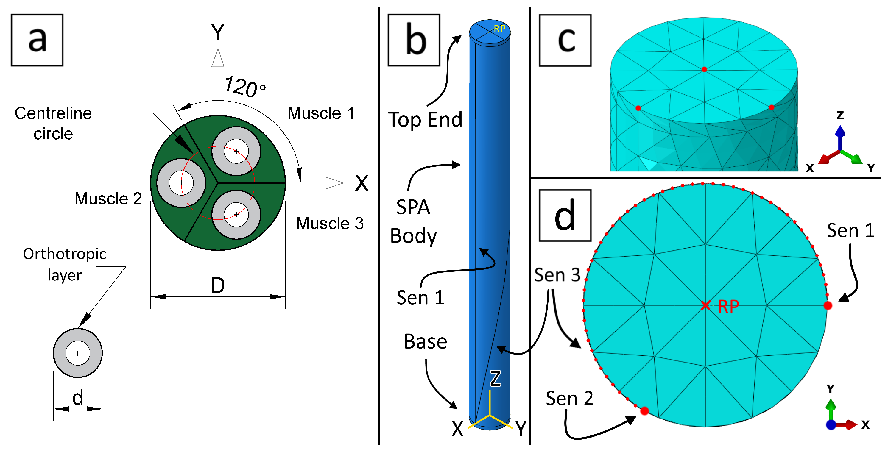
Inspired by [9], our multi-muscle soft pneumatic actuator (SPA) consists of 3 pneumatic muscles. The circular cross-section lies in the XY plane where the geometric centre is located at the origin. The actuator height is along the + z - a x i s , and the muscles are 120 apart, Figure 12a. The first muscle is located in the 1st quadrant, the second muscle is located at the x - a x i s , and the third muscle is located in the 4th quadrant. This configuration provides the ability to generate a bending movement in the XZ plane, i.e., ϕ = 0 , by activating the minimum number of muscles, i.e., the second muscle only. Each muscle was simulated as a silicone tube with a diameter d = 8 mm and a thickness of 2 mm. The external surface of each muscle was reinforced by the orthotropic layer. The SPA body was simulated as a silicone structure as well (coloured in green to differentiate it from the muscles) with a diameter D = 22 mm and divided into 3 sectors to mark its centreline, as described in Section 4.4 below.
The SPA consists of three parts, two stainless steel 18 / 8 discs, base and top end with a 2  mm thickness each, and a silicone body with a height of 250 mm, as shown in Figure 12b. The stainless steel 18 / 8 has a density of 7930 Kg/m 3 , a Young’s modulus E 1 = 193 GPa, and a Poisson’s ratio ν 12 = 0.305 . The base was fixed, and the top end was free to move and rotate in all directions. In Abaqus, the STRI65 element type was used to model the orthotropic layer. It is a 6-node triangular thin shell element, using five degrees of freedom per node. Similarly, the C3D10HS element type was used to model the silicone and stainless steel parts. This element type is a 10-node general-purpose quadratic tetrahedron with improved surface stress visualisation.
A pressure load ( p 1 , p 2 , and p 3 ) can be applied to each muscle individually to generate extension, bending, and rotation movements. For twisting movement, a moment M can be applied at the SPA free end. Since the C3D10HS element type has translation DOFs only, the moment M could not be applied on the top surface directly. Instead, we defined a reference point (RP), Figure 12b,d, in space and connected it to the edge of the top end using a continuum distributing coupling constraint. Applying the moment M on RP generated the required twist. Anticlockwise moments were positive since all rotations in Abaqus are following the right-handed rule.

4.4. Centreline and Soft Sensors’ Length

The SPA body was divided into 3 sectors, Figure 12a and Figure 13c, to create an edge that marked the centreline. Furthermore, we partitioned the surface of the SPA at specific locations to generate edges that represented the three soft sensors, Figure 12b. The first sensor had a straight path, where v s 1 = v e 1 = 0 . The second sensor had a straight path as well, where v s 2 = v e 2 = 4 3 π . The third sensor had a spiral path, where v s 3 = 0 and v e 3 = 4 3 π , as shown in Figure 12d. The sensors covered the entire length of the SPA body, i.e., start from the base and stop at the edge of the top end. We then created 4 node sets along the centreline and the edge of each soft sensor after meshing the SPA.
The locations of the sensors were selected strategically to provide enough information about the actuator’s entire range in extension, bending, rotation, and twist. From simulation results, we extracted the Cartesian coordinates of each node in these sets at every time frame using Python code. The Python code exported the results to MATLAB in order to calculate the required results and compare them with the mathematical model. The Python code (MultiMuscles_data_extract.py) that extracted the data to MATLAB is provided in the supplementary materials.
To calculate the centreline and soft sensors’ length in MATLAB, we represented each data set as B-spline curves [65]. Splines are piecewise polynomial functions that can describe complex trajectories using few variables. The B-spline curves can be used in path approximation and the result is a smooth curve instead of a piecewise polygonal curve with sharp peaks. The advantage of this approximation is the independence from the FEA mesh size.
A B-spline curve with p-degree is formed by a linear combination of B-spline basis functions, and defined as [66]
B ( g ) = P 0 N 0 , p ( g ) + P 1 N 1 , p ( g ) + + P n N n , p ( g ) = i = 0 n P i N i , p ( g ) .
where P i are the control points, and N i , p ( g ) are B-spline basis functions of degree p and defined as
N i , p ( g ) = g g i g i + p g i N i , p 1 ( g ) + g i + p + 1 g g i + p + 1 g i + 1 N i + 1 , p 1 ( g ) ,
where g i , i = 0 , 1 , 2 , , n + p + 1 are the B-spline knots, and g i g i + 1 . Similar to (11), the length of B ( g ) can be calculated by integrating the norm of its derivative
l b = 0 g n + p + 1 B ( g ) 2 d g ,
where B ( g ) is a B-spline curve of degree p 1 , derived as
B ( g ) = d d g B ( g ) = i = 0 n 1 p g i + p + 1 g i + 1 P i + 1 P i N i + 1 , p 1 ( g ) .
Equation (28) can be integrated numerically to calculate the length of the centreline and the three soft sensors at each time frame.

4.5. Centreline Curvature

The model (18) that calculates the length of soft sensors was derived for a constant curvature actuator as stated earlier. Moreover, the curvature value was required for the sake of comparison between the mathematical model and Abaqus results. Therefore, we calculated the SPA curvature at each time frame.
Let γ c ( t ) = x 1 ( t ) , y 1 ( t ) , z 1 ( t ) be a parametric equation defining the centreline curve in the Cartesian coordinates at any given time t. Assuming γ c ˙ is defined, differentiable, and nowhere equal to the zero vector, the curvature can be derived as [67,68]    
κ = γ c ˙ × γ c ¨ γ c ˙ 3 ,
where × denotes the vector cross product. Simplifying gives the curvature as
κ = z ¨ 1 y ˙ 1 y ¨ 1 z ˙ 1 2 + x ¨ 1 z ˙ 1 z ¨ 1 x ˙ 1 2 + y ¨ 1 x ˙ 1 x ¨ 1 y ˙ 1 2 x ˙ 1 2 + y ˙ 1 2 + z ˙ 1 2 3 / 2 .
Assuming a position tolerance of 0.001 mm for the top end, the minimum curvature to satisfy this tolerance can be calculated using simple trigonometric equations. For an actuator with a flexible length of 250 mm, the minimum curvature is κ m i n = 3.2 × 10 8 mm 1 . The actuator is considered straight for any curvature below this limit. In MATLAB, representing γ c as a B-spline of class C 2 ensures a smooth curve for calculating the first and second derivatives numerically. The required Cartesian coordinates were extracted using the procedure described in Section 4.4 above.

4.6. Bending, Rotation, and Twist Angles

The Kabsch algorithm [69] was used to calculate the bending θ , rotation ϕ , and twist ψ angles of the actuator. This algorithm calculates an optimal rotation matrix R k that minimises the root-mean-square error e k between two paired sets of 3D points, A k and B k . For our SPA, the two sets had the same points (nodes), where the first set A k was at the SPA initial position, and the other set B k was at any given time. The first set A k consisted of 3 nodes located at the SPA’s top edge surface, Figure 12c. One node was located at the centre of the surface, the second node was located at the + x - a x i s , and the last node was located at the + y - a x i s . Tracking the coordinates of these three nodes at any given time provided the required data sets, A k and B k , for Kabsch’s algorithm.
Given two 3D point sets A k , B k R 3 × 3 , the transformation is
B k = R k A k + t k + N k ,
where t k is the translation matrix, and N k is the noise matrix.
The root-mean-square error is
e k = i = 1 3 R k A k i + t k B k i 2 ,
in which the vectors A k i , B k i R 3 . Both R k and t k can be calculated by minimising e k . To achieve that, let us find the centroid of each data set
c e n A = 1 3 i = 1 3 A k i , c e n B = 1 3 i = 1 3 B k i ,
then recentre both data sets so that both centroids are at the origin to eliminate the translation component, leaving us with only the rotation to deal with. The root-mean-square error becomes
e k = i = 1 3 R k c e n A c e n B 2 .
The optimal rotation and translation can be found by calculating the singular value decomposition (SVD) of a cross-covariance matrix H k as follows
H k = A k c e n A B k c e n B T = U Σ V T ,
which gives
R k = V 1 0 0 0 1 0 0 0 d k U T , t k = c e n B R k c e n A ,
where d k = s i g n d e t V U T is a correction factor to ensure a right-handed coordinate system. The translation matrix t k was irrelevant to our current model, and we reported it as a reference for any future analysis.
Now, converting the rotation matrix R k to the Euler rotation angles r 1 , r 2 , r 3 around the Cartesian axes requires determining the proper rotation order. Figuring the proper order provides the correct conversion from the Euler to the SPA angles. Starting from the SPA initial (straight) position, both rotation ϕ and twist angles ψ are rotating around the z - a x i s , while bending angle θ is rotating around the y - a x i s . This order is denoted as Z Y Z . However, for twist only, this order generates a singularity, and the alternative order is X Y Z which eliminates rotation, i.e., ϕ = 0 , since it is irrelevant at the initial position.
When the SPA curvature κ κ m i n , i.e., a Z Y Z rotation order, the Euler angles can be calculated [70] using R k as follows
r 1 = a r c t a n R k 23 R k 13 , r 2 = a r c t a n 1 R k 33 2 R k 33 , r 3 = a r c t a n R k 32 R k 31 ,
and for κ < κ m i n , i.e., an X Y Z rotation order, the Euler angles are
r 1 = a r c t a n R k 23 R k 33 , r 2 = a r c t a n R k 13 1 R k 13 2 , r 3 = a r c t a n R k 12 R k 11 .
Equations (38) and (39) can be implemented directly in MATLAB, or use the direct cosine matrix to Euler’s function (dcm2angle) after inverting rotation angle R k to change the rotation from extrinsic to intrinsic. Finally, the SPA angles are calculated as
ϕ = r 1 , θ = r 2 , ψ = r 1 + r 3 .
Notice that twist angle ψ is the summation of the two Euler angles r 1 and r 3 . This is due to the fact that rotating the actuator around the z - a x i s causes the top end face to rotate [15] in the opposite direction since the base is fixed. Therefore, ψ = 0 if there is no external or additional twist.

5. Simulation Results and Discussion

The purpose of this simulation was to verify the mathematical model of (18). It represents the soft sensor’s length when attached to the surface of a toric-shaped soft actuator as mentioned earlier in Section 2.2. To achieve that, we introduced a new approach to simulate the reinforcement layer, Section 4.2 above. The validation of our new approach is presented in the following section.

5.1. Single-Muscle Extension Test

In order to validate our new approach, we conducted an extension test in Abaqus and compared the change in length with previously published results by [43]. Our simulated sample, Figure 14a, consisted of a single pneumatic muscle that had a thickness, outside diameter, and initial length of 2 mm, 16.7 mm, and 165 mm, respectively. These were the same dimensions as the sample in [43] that we used in our comparison.
The base was fixed and the top end was free to move. Both base and top surfaces were covered with a skin modelled as a piece of paper [64] with a density of 750 kg/m 3 , a Young’s modulus E 1 = 6.5 GPa, and a Poisson’s ratio ν 12 = 0.2 . This paper skin prevented the surfaces from deforming radially but maintained flexibility at the connection edges. We used the same silicone material, Elastosil M4601, and applied the same pressure value of 62.05  kPa in our simulation. We used an approximate global mesh size of 2.0 as an optimum selection between accuracy vs. computation time. We created a circumferential nodal path, Figure 14b, to compare its length at 0 % and 100 % pressure. This was a required task to ensure there was no change in the pneumatic muscle diameter d. We extracted data points from the results in ([43], Figure 2a at a 0 fibre angle) and plotted them against our simulation results as shown in Figure 14c. The results proved that our reinforcement layer was close enough to experimental data with an error < 0.5%. Furthermore, the circumferential path length did not change during the extension, which proved the validity of our reinforcement layer as well. The muscle extended by about 17 % at full pressure which was within the 20 % extension limit with a neglected diameter change, as discussed earlier in Section 4.1. Comparatively, [43] reported an approximate diameter change of 1.5 % in their test at full pressure which could be neglected as well. Finally, the Python code (SingleMuscle.py) that generated our Abaqus model shown in Figure 14a,b is provided in the supplementary materials.

5.2. Multiple-Muscle Actuator

We used an approximate global mesh size of 5.0 as an optimum selection between accuracy vs. computation time. The simulation was a ‘static, general’ procedure using the Abaqus/Standard solver, and the total time was 1 s. We conducted several tests to generate extension, bending, rotation, and twisting movements in various combinations. The simulation values of pressures p 1 , p 2 , p 3 , and moment M are listed in Table 1 for all the simulation scenarios. The initial lengths of the centreline, first, second, and third sensors were 250 mm, 250 mm, 250 mm, and 254.2 mm, respectively. Finally, the Python code (MultiMuscle.py) that generated our Abaqus model shown in Figure 12 and Figure 13 is provided in the supplementary materials.

5.2.1. Simulation Scenarios

For the first simulation scenario, bending and extension, the higher load was given to the second muscle. The SPA bent in the XZ plane, and the curvature reached around 0.0052 mm 1 , Figure 15(a1,b1). Both rotation ϕ and twist ψ angles were zero approximately while bending θ angle reached 76.3 deg, Figure 16(a1). The centreline length extended 4.7 % , Figure 16(b1). For the second scenario, the higher pressure p 3 caused the SPA to rotate an average of 60 deg anticlockwise around the + z - a x i s along with bending and extension, as indicated by the projection of the SPA on the XY plane, Figure 15(a2). The bending angle θ and curvature were 82.5 deg and 0.0055 mm 1 , respectively. The centreline length extended by 7.3 % , which was more than its extension in the first scenario. This extra extension was expected since the total pressure, p 1 + p 2 + p 3 , had increased. Similar to the first scenario, the twist angle ψ was approximately zero since there was no twisting moment, Figure 16(a2).
The third scenario involved adding a twisting moment M to the second scenario configuration. We repeated the third scenario three times by using different moment M values, 15, 30, and 45 N·mm. The results of the latter is shown in Figure 15 and Figure 16. The centreline length extended by an average of 7.4 % in each of these three simulations. The twisting moment caused an arching in the SPA centreline in which the bending was no longer within a plane, Figure 1b. This arching is clearly visible via the projection of the SPA on the XY plane in Figure 15(a3). The amount of this arching was directly proportional to the moment M value. We believe the dissimilar pressure loads in the muscles was the main cause for this arching. That means arching is expected whenever there is a twisting moment along with the bending, generally speaking. However, different boundary conditions at the top end may generate different behaviours under moment loading. The investigation of this arching behaviour was beyond the scope of this study. The twist angle ψ reached 38.7 , 80.2 , and 121.7 deg after applying a moment M of 15, 30, and 45 N·mm, respectively. Moreover, the rotation angle ϕ increased noticeably from its initial value, from 60.6 to 76.4  deg for M = 45 MPa, due to the arching, Figure 16(a3). This increment was expected since the angles were calculated using the three tracking nodes at the top end surface, Figure 12c.
The fourth and final scenario involved twist and extension. The purpose was to study the effect of twist on the sensors’ sensitivity [71] and demonstrate the advantage of our spiral sensors model (18). We restricted the translation of the centreline in both the x- and y - a x e s . The SPA extended by 10 % along the + z - a x i s by applying equal pressure loads at its three pneumatic muscles, i.e., p 1 = p 2 = p 3 = 0.2 MPa. Additionally, the SPA rotated freely in the anticlockwise direction around the + z - a x i s by applying a moment of M = 45 N·mm. The twist ψ angle reached 130.9 deg, Figure 16(a4). Both bending angle  θ and rotation angle  ϕ were zero as expected, since the SPA did not bend, i.e., curvature κ κ m i n .

5.2.2. Curvature Constancy

Before calculating the soft sensors’ length, we inspected the simulation results of the SPA curvature. The goal was to find whether it was a constant or a variable curvature in each simulation scenario. However, the curvature was neglected for the fourth scenario since there was no bending. We calculated the curvature using (31) at each time frame. Figure 15(c1–c4) show the curvature across the SPA length at the final time frame for each scenario. The fluctuation was expected due to the first and second derivative even when using a B-spline to smooth the discrete results of the Abaqus model. Apparently, the curvature was fluctuating around a certain value across the length, which indicated it fulfilled the required constancy condition. We calculated the probability density function (PDF) of the curvature to confirm it had a normal distribution, Figure 15(d1–d4), as an indication of the constancy. The mean value of the normal distribution is shown in Figure 15(c1–c4) as a dashed red line as a comparison with the curvature. Since the SPA was straight in the fourth scenario, i.e., curvature κ < κ m i n , the mean of the normal distribution was expected to be less than κ m i n as well. The curvature values shown in Figure 15(b1–b4) are the mean of the normal distribution at each time frame. These values were used in (18) to calculate the length of the three soft sensors at each time frame for the sake of comparison with the Abaqus results.

5.2.3. Length of Soft Sensors

The length of each soft sensor may be extended or reduced based on the actuation direction and the location of each sensor, i.e., v s i and Δ v i . In our simulation, we assumed the sensors were able to measure both extension and reduction, which could be achieved by using pre-stretched sensors as an example. In the first scenario, the length of both second and third sensors increased while it decreased for the first sensor, Figure 16(b1). For the second scenario, Figure 16(b2), the second sensor extended more than the other two sensors since the SPA bending occurred in the opposite direction of the second sensor, i.e., ϕ 60  deg.
The arching in the third scenario caused a noticeable increase in the error, especially for the third sensor, Figure 16(c3). The spiral geometry of the third sensor made it more sensitive to the arching than the first and second sensors. Yet, our mathematical model (18) was able to maintain a high accuracy despite the unmodelled arching. The length errors of the third sensor with respect to the Abaqus results were 0.7 % , 1.3 % , and 1.5 % approximately at twisting moments M = 15 , 30, and 45 N·mm, respectively. The latter is shown in Figure 16(c3). Furthermore, the relations between curvature, centreline, and sensor length vs. time were linear in both first and second scenarios since there was no arching, Figure 15(b1,b2) and Figure 16(b1,b2). Some of these relations started exhibiting nonlinear behaviours in the third scenario, Figure 15(b3) and Figure 16(b3), which can be investigated in future work to gain more insights into the arching. The advantage of including twist in the length model of soft sensors is discussed in Section 5.2.4 below.
A distinguished trend for the length error can be seen in the third scenario, Figure 16(c3), in which the error rate, i.e., the slope of the error curve, increased then decreased for all sensors. We believe this trend is related to the arching effect and has a direct relationship with twisting moment M value. A further change in the error rate can be seen in the results of the second sensor, in which the rate increased again, Figure 16d–f. We believe such further change is related to the loading scenario. The second sensor was located between the first and second muscles in which the higher pressure was applied, i.e., p 1 and p 2 . The combined effect of the arching and the second sensor location led to such a distinguished trend in the length error. A further investigation is required to study how much the error values can reach and what trends they would exhibit under different loading scenarios.
The fourth and final scenario was designed to show the relation between the twist angle ψ and the sensors’ length. The extension of the soft sensors was a combination of the overall SPA’s extension and twist, Figure 16(b4). The third sensor exhibited more change in length since its spiral geometry had more sensitivity to the twist. Identical results were expected for both first and second sensors; however, there was a minor difference in the length errors, which we believe was due the accuracy of the Abaqus model, Figure 16(c4). Nonetheless, both errors were very small and would most likely be neglected in experimental or real-life applications. For all scenarios except the third, the length error of any sensor did not exceed 0.33 % , Figure 16(c1,c2,c4), which proved the validity and high accuracy of our model (18).

5.2.4. Twist in Length Model

To demonstrate the advantages of including the SPA twist in our model (18), we calculated the length of the first and second sensors by omitting the twist from our model, i.e., ψ = 0 at all times, in both third and fourth scenarios. We selected the first and second sensors since they were straight at the initial position. Omitting the twist for straight sensors simplified our model to one resembling models from previous studies in the literature. A good example can be seen in the study of Della Santina et al. [15] in which the four arcs in their model could be treated as four soft sensors.
By comparing with the Abaqus results, Figure 16d–f show the percentage of length error when omitting the twist in the third scenario at twisting moments M = 15 , 30, and 45 N·mm, respectively. The arching in the third scenario caused a deviation of Δ ϕ = 11.3 , 21.2 , and 27.4 deg in rotation angle ϕ , Figure 16g, at a twisting moment M = 15 , 30 and 45 N·mm, respectively. Another deviation is observed in bending angle θ , not shown, which explains the slight difference between the mean and the curvature trend after 80 % of the SPA length in Figure 15(c3). We believe that arching is one of the reasons for the error difference between including or omitting the twist. However, analysing the effect of arching was beyond the scope of this study.
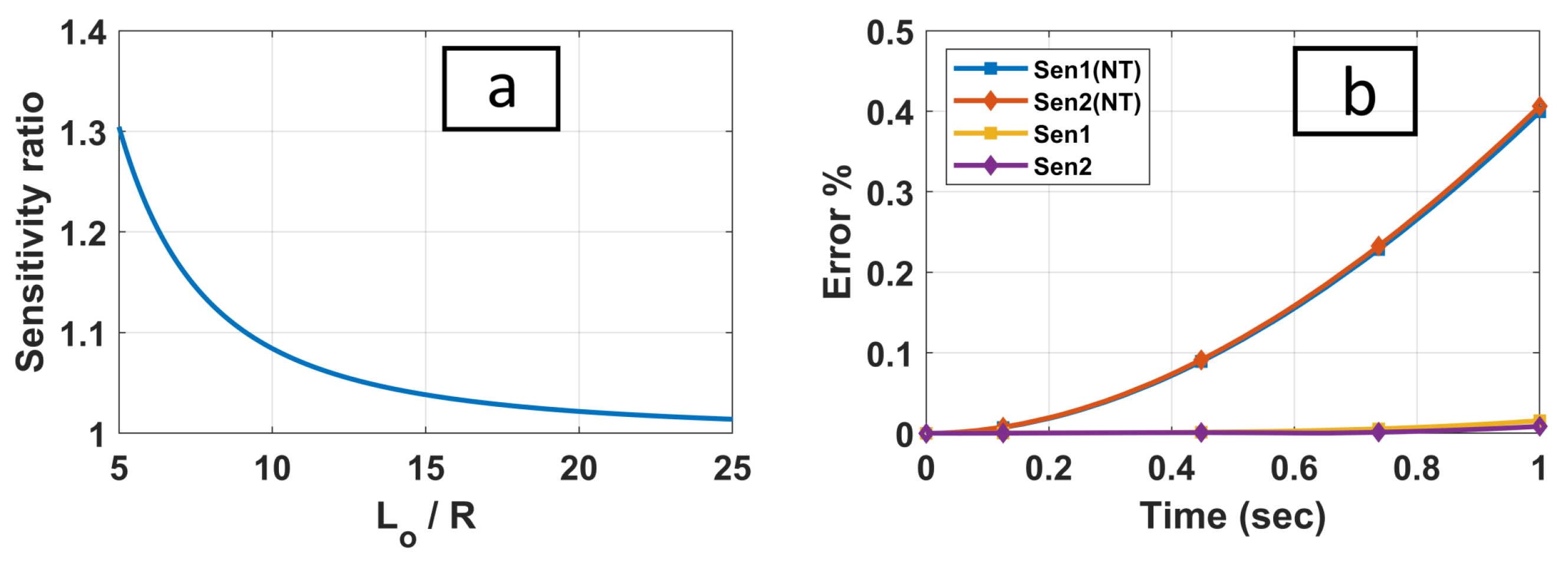
The first sensor exhibited a larger error based on its location, the SPA state (i.e., bending, rotation, and extension), and the amount of twisting moment. For the third scenario, the first sensor error reached 4 % when omitting the twist compared to a 0.55 % actual error in our model (18) with respect to the Abaqus results, Figure 16f. Furthermore, for the fourth scenario, the error when omitting the twist was 0.4 % and 0.41 % for the first and second sensors, respectively, Figure 17b, compared to the negligible error values ( 1.6 × 10 2 % and 8.5 × 10 3 % , respectively) of our model (18) with respect to the Abaqus results. This is a massive difference and proves the advantage of including a twist in the soft sensors’ length. Additionally, including a twist in the length model provides the ability to model spiral strain sensors. Moreover, with a twist in the model, the SPA state as well as the unknown twisting moment M can be estimated using one of the state estimation algorithms such as Kalman filtering [72]. It is important to highlight that the first and second sensors should have had similar error values in the fourth scenario since there was no bending or rotation. The difference between their errors, 0.01 % , was insignificant compared to the error values themselves when omitting the twist, i.e., 0.4 % and 0.41 % . Instead, the difference was significant compared to the negligible errors of our model (18), i.e., 1.6 × 10 2 % and 8.5 × 10 3 % . However, the latter errors were very small and can be neglected as they were related to the selected FEA mesh size.

5.2.5. Sensitivity

A sensor’s sensitivity is an indication of how much the output is changing when the measured input quantity changes [71]. For an extension simulation, both spiral and straight sensors are measuring the same input quantity which is the change in the SPA centreline length. Therefore, the sensitivity ratio of spiral to straight sensor can be simplified to be the length ratio. Simply, for a given SPA, longer sensors will have more sensitivity to the change in the centreline length. Furthermore, the spiral sensor’s length increases when the SPA’s cross-section radius increases too.
To demonstrate this concept, we plotted the spiral to straight sensor sensitivity ratio vs. the SPA length-to-radius ratio L o / R at the SPA initial position, Figure 17a. The straight sensor had a similar geometry to either first or second soft sensor in our FEA simulation. The spiral sensor had a similar geometry to the second soft sensor in our FEA simulation, i.e., Δ v i = 4 3 π . Our SPA had a length-to-radius ratio of 22.7 approximately, which gave a sensitivity ratio of 1.017 . Yet, with such a small difference in sensitivity, the spiral sensor had a change in length noticeably bigger than the straight sensors, Figure 16(b4). Therefore, using spiral sensors may provide some advantages based on the SPA and the sensor configurations as well as the testing scenarios. The spiral sensor’s sensitivity increases when using sensors with a bigger spiral span Δ v i or an SPA with a smaller length-to-radius ratio L o / R . The optimum L o / R ratio is based on the application requirements [73] and the designing preferences.

5.3. Model Validation

In addition to the earlier validation presented in Section 5.1, a subsequent validation of our model (18) is required to ensure its accuracy. Conducting experimental tests involves several tasks, such as designing the actuator and the sensors, designing a controller, and calibrating the data acquisition and motion capture systems. These tasks can vary from one test to another. Thus, in order to validate our model (18) and illustrate its flexibility, we chose to compare our theoretical results with previously published experimental results. Our literature review, conducted within the scope of this study, revealed a lack of relevant studies concerning PCC-based soft actuators, with the exception of [25,26,27], as discussed in Section 1.3 above.
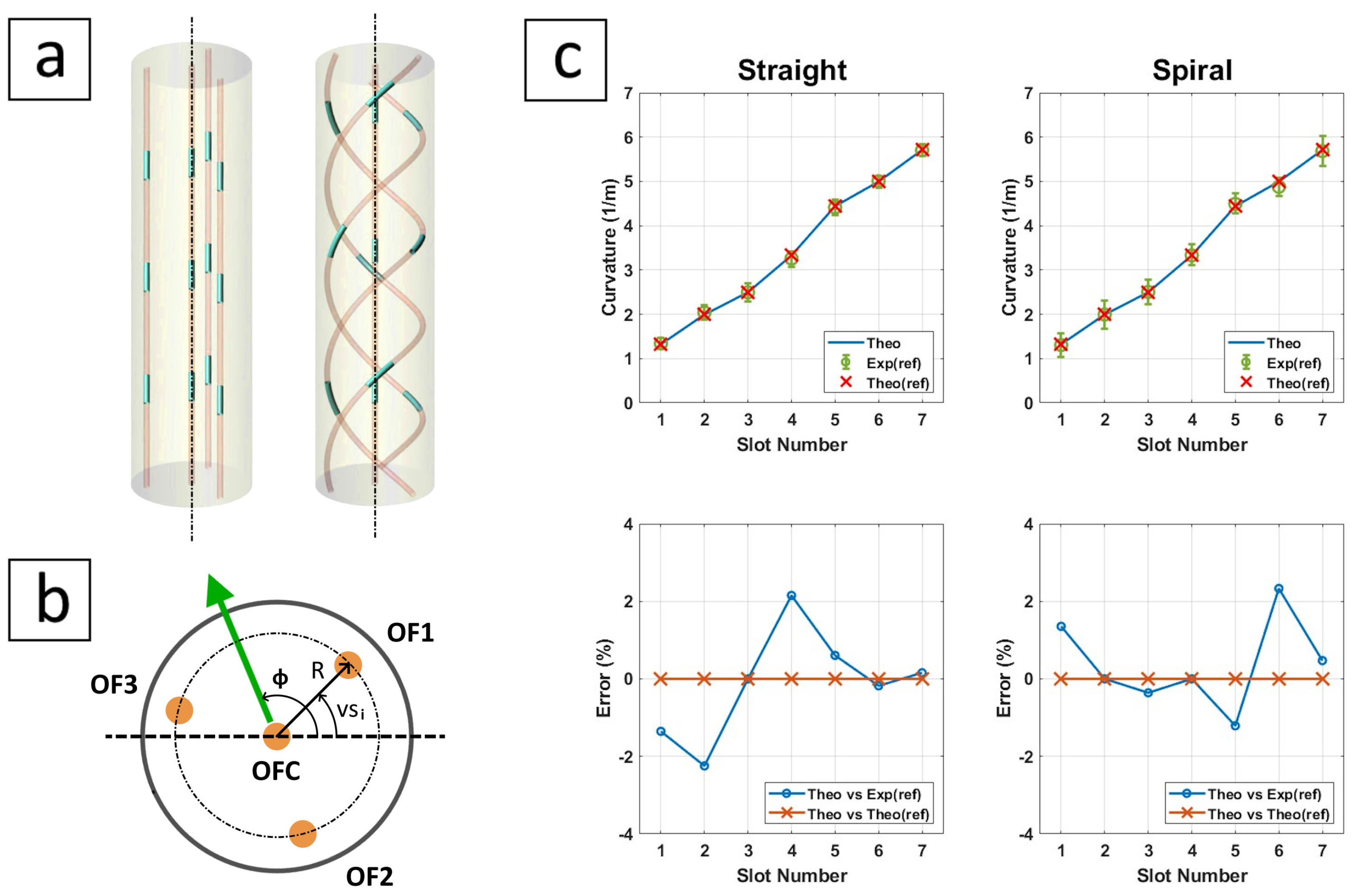
Nonetheless, other studies can be used as long as the PCC model is maintained during the experimental tests. One such study is that conducted by F. Khan et al. [24], and it involved three different tests, which were bending, twist, and deformation reconstructions. The test samples were two multi-core optical fibres, one with straight cores and the other with spiral cores. Each sample had three peripheral optical fibre cores O F 1 , O F 2 , and O F 3 spaced 120 deg apart, and a fourth central core O F C to be used for temperature variation compensation, as shown in Figure 18a,b. The cores in both samples contained multiple sets of FBG sensors inscribed in them and connected to an interrogator that provided the light source as well as analysed the reflected spectrum for the purpose of measuring the local strain in each FBG sensor.
The peripheral optical fibres were located at a radius of 35 μ m. The two samples had a sensorised length of 115.5 and 175 mm for the straight and spiral fibres, respectively. The spiral fibres had 50 turns per unit length. We modelled the optical fibres as three straight sensors and three spiral sensors. Both straight and spiral sensors were located at a radius of R = 0.035 mm. The three individual sensors in both straight and spiral samples had a starting coordinate of v s i = 0 , 2 3 π , 2 3 π . The straight sensors had a coordinate difference of Δ v i = 0 , while the spiral sensors had a coordinate difference of Δ v i = 35 2 π based on the number of turns per unit length.
For the bending test, the authors used a test bench made of an acrylic board that contained seven slots with different curvatures ranging from 1.33 to 5.71 m 1 . This test resembled the first or second simulation scenario discussed in Section 5.2.1 above based on the rotation ϕ angle. We extracted the curvature values and the corresponding measurements from the published results ([24], Figure 5a) and used the curvature values to calculate the strain results using our model (18) for both the straight and spiral sensors. Then, we calculated the theoretical curvature results using ([24], Equation (7)) in order to compare them with the authors’ model and experimental results. The rotation angle could be set to ϕ = 0 since its value would not change the results given that ([24], Equation (7)) calculates the magnitude of the curvature vector and neither samples had fixed ends. The comparison results are shown in Figure 18c, and the MATLAB code (FBG_SNA2021.m) along with the extracted data (FBG_SNA2021_data.m) that were used to generate the results are provided in the supplementary materials.
The comparison indicates that the theoretical results of our model (18) and the reference study [24] match properly. To clarify, the bending model in [24] is considered a simplified model compared to our model (18) since the centreline length extension, rotation, and twist are excluded. The comparison with the experimental results shows a good match within a mean error of less than ± 2.4 % , keeping in mind that this error includes both manufacturing and measurement inaccuracies. Furthermore, the comparison confirms the flexibility of our model (18) for representing various tests as long as the PCC model is maintained.
For the twist test, the authors used a linear model ([24], Equation (8)) that related the twist angle to the strain. This model included a material constant, denoted as ‘G’ in [24], and it was calculated experimentally. Such an approach has limitations when it comes to representing the twist, considering the non-linear nature of the strain vs. twist angle [74]. In addition, testing bending along with the twist requires calculating the material constant for each curvature. The large error that can be seen in their results of the twist test confirmed our concern ([24], Figure 6a,b). Finally, the deformation reconstruction test was outside the scope of our study.

5.4. Limitations and Applications

As stated earlier, our model (18) is limited to (1) PCC SPAs in which (2) the sensors are located in one or multiple sensing layers. These sensing layers have constant cross-sectional diameters across the SPA segment length. The actuation of the SPA segment should not change these diameters, i.e., the radial expansion or contraction in each sensing layer is minimal and neglected at all times.
We demonstrated the accuracy of our model (18) using a multi-muscle SPA, Section 5.2, that satisfied both of these limitations. Three sensors were attached to the outer surface of the SPA in which the radial expansion was restrained by using braided sleeves. Alternatively, the sensors can be placed closer to the centreline of the SPA. One example can be seen in [25], where the authors used FBG sensors to detect the shape of the SPA. The sensors were located on the internal surface of the SPA, which had a constant cross-sectional diameter across the length and a neglected radial expansion. Our model (18) can add a twist measurement to their actuator.
Complex geometries such as bellow-type SPAs [75] can be sensorised based on our model (18) as well. The SPA segment of [75] was designed to follow the PCC model. The sensors "can be" placed in their constraining layer at a certain diameter to add bending, rotation, and twist measurements if required. PneuNet actuators, on the other hand, produce planar movement, i.e., bending only. Planar movement eliminates the need to have rotation and twist measurements. A simple curvature sensor is enough to measure the bending [76]. Moreover, not only soft actuators but other PCC continuum actuators can utilise our model (18) too. A good example is nitinol-based actuators, in which FBG sensors were embedded in grooves on the outer surface [28] or attached to the outer surface using adhesive [77].
The FEA simulation in our study provided an in-depth verification of the accuracy of our model (18). We selected an FEA simulation since it is widely used in soft robotics research [78]. In addition, the experimental validation presented in Section 5.3 above confirmed the accuracy of our model (18) and its flexibility to represent various tests that align with the two limitations above. In addition to this, some interactions with the environment are still possible as long as they do not validate the PCC assumption. As an example, the actuator can be controlled to interact with the surrounding environment [79] or designed to perform underwater manipulation tasks [80] despite the forces applied by the water on the actuator surface.
However, to examine the full potential of our model (18) in real applications, further aspects need to be considered and addressed, such as the soft actuator design, the type of soft sensors, the measurement hysteresis, nonhomogeneous strains, the limits of the motion capture system, the calibration process, etc. These aspects have measurement errors as well. Providing answers to these aspects and determining the overall accuracy would require conducting experimental testing, which was outside the scope of this study.

6. Conclusions

A PCC-based soft actuator can be subjected to extension, bending, rotation, and twist. Previous studies that modelled the length of straight strain sensors may provide enough capability to sense extension, bending, and rotation. However, a twist can generate errors in measurements if not modelled mathematically. Despite the limitation of the PCC model, we provided the ability to represent spiral sensors as well as SPA twists. We utilised the concepts of geodesics and covering spaces as an approach to derive a simplified and straightforward model compared to the approach presented in [33].
We built a simplified FEA model for the SPA and designed simulation scenarios to verify the accuracy of our model (18). We suggested using an orthotropic layer as a technique to model the reinforcement of the pneumatic muscles. We then validated our suggested technique by comparing the results of a single-muscle extension with previously published results. Our reinforcement technique can reduce the FEA simulation time significantly since it eliminates the need to use contact interactions in Abaqus. Furthermore, we provided a procedure for calculating the length of the centreline and soft sensors from our FEA model by utilising B-splines to smooth discrete results. Finally, we implemented the Kabsch algorithm to calculate bending ( θ ), rotation ( ϕ ), and twist ( ψ ) angles from our FEA model. Collectively, our FEA simulation technique can help other researchers to develop customised FEA models, study SPA movements extensively, save significant simulation efforts and resources in both pre- and post-processing stages, and expedite data extraction to MATLAB by utilising the codes we developed in our study.
The results proved the ability of our model (18) to represent straight and spiral sensors under various testing scenarios. The error in the length measurements of the soft sensors did not exceed 0.33 % in both the first and second simulation scenarios. Applying a twisting moment at the free end generated arching in the SPA. The error in the length measurements did not exceed 1.5 % despite the arching, and the PCC approximation was nonetheless still applicable. The accuracy of our model (18) depends on the applicability of using the PCC model in any certain application. Higher twisting moments can cause bigger arching and void the suitability of using the PCC model. Compared to the CRM and PCS models, the PCC model is considered a favourable choice for real-time control due to its simplicity in kinematic modelling [12]. However, justifying the suitability of using the PCC model in any application is outside the scope of this study.
By comparing the excluding vs. including twist in the soft sensor model, we found that twisting of the free end caused a 7.3 -time larger error in the third scenario and a 48.2 -time larger error in the fourth scenario. Such larger errors confirm the advantage of using our model (18) for representing both the straight and spiral soft strain sensors in various configurations. Spiral sensors have a higher sensitivity compared to straight sensors within the same SPA since they are longer. Our model (18) provides the ability to use them when developing soft sensing applications. This sensitivity can be enhanced by increasing the spiral sensor length by increasing the spiral span Δ v i or the SPA length-to-radius ratio L o / R . Lastly, we provided experimental validation to our model (18) by comparing the theoretical results with previously published results to demonstrate its accuracy and flexibility. We then discussed the limitations of our model (18) and addressed several possible applications.
Our mathematical model, FEA model, and testing scenarios provide a new tool to improve proprioceptive sensing of several PCC-based soft actuators and potentially lead the way for future implementations, such as in real-time control applications. Further investigations are required to study the arching and provide suggestions to enhance our model (18) for better accuracy. Also, our model (18) can be used in state estimation algorithms to estimate not only the SPA state in 3D space but the twisting moment as well, if its value is unknown [72]. The state estimation can be extended further to include experimental sensing measurements [81] after estimating the state and measurement noise covariance matrices.   

Supplementary Materials

The following Python and MATLAB codes can be downloaded at: https://www.mdpi.com/article/10.3390/robotics12060164/s1, single-muscle actuator (SingleMuscle.py), multi-muscle actuator (MultiMuscle.py), data extraction (MultiMuscle_data_extract.py), experimental validation (FBG_SNA2021.m), and (FBG_SNA2021_data.m) as a single archive file. Also, the source codes can be downloaded from our GitHub repository as per the details provided in the data availability statement below.

Author Contributions

Conceptualisation, A.A.-A. and P.S.; methodology, A.A.-A.; software, A.A.-A.; validation, A.A.-A. and P.S.; formal analysis, A.A.-A.; writing—original draft preparation, A.A.-A.; writing—review and editing, A.A.-A., P.S., H.K. and S.S.; supervision, S.S. All authors have read and agreed to the published version of the manuscript.

Funding

This research received no external funding.

Data Availability Statement

We have made the source codes for the simulations conducted in this study available on our GitHub repository: https://github.com/abd-alaz/spiral-sensors (accessed on 22 November 2023). Interested readers can access and download the codes for a closer examination of the implementations and methods employed. The codes are open-source and provided under the GNU General Public License v3.0, allowing for academic and non-commercial use.

Acknowledgments

The authors would like to express their gratitude to MD Nazmul Hassan and Omar Al-Kubaisi form The University of Sydney in Australia for their comments regarding orthotropic layer, Jennifer Case from the National Institute of Standards and Technology (NIST) in USA for her comments regarding proprioceptive sensing, and Fouzia Khan from Thermo Fisher Scientific in the Netherlands for her help in explaining the study presented in [24].

Conflicts of Interest

Author Peter Stadler was employed by the company e:fs Techhub GmbH. The remaining authors declare that the research was conducted in the absence of any commercial or financial relationships that could be construed as a potential conflict of interest.

Abbreviations

The following abbreviations are used in this manuscript:
CRMCosserat rod model
DOFDegree of freedom
FEAFinite element analysis
FBGFibre Bragg grating
IMUInertial measurement unit
CLDConstant centreline length (design)
NCDNoncompressible inner surface (design)
PCCPiecewise-constant curvatures
PCSPiecewise-constant strain
PDFProbability density function
PETPolyethylene terephthalate
SPASoft pneumatic actuator

References

  1. Bao, G.; Fang, H.; Chen, L.; Wan, Y.; Xu, F.; Yang, Q.; Zhang, L. Soft Robotics: Academic Insights and Perspectives through Bibliometric Analysis. Soft Robot. 2018, 5, 229–241. [Google Scholar] [CrossRef] [PubMed]
  2. Polygerinos, P.; Correll, N.; Morin, S.A.; Mosadegh, B.; Onal, C.D.; Petersen, K.; Cianchetti, M.; Tolley, M.T.; Shepherd, R.F. Soft Robotics: Review of Fluid-Driven Intrinsically Soft Devices; Manufacturing, Sensing, Control, and Applications in Human-Robot Interaction. Adv. Eng. Mater. 2017, 19, 1700016. [Google Scholar] [CrossRef]
  3. Mustaza, S.M.; Elsayed, Y.; Lekakou, C.; Saaj, C.; Fras, J. Dynamic Modeling of Fiber-Reinforced Soft Manipulator: A Visco-Hyperelastic Material-Based Continuum Mechanics Approach. Soft Robot. 2019, 6, 305–317. [Google Scholar] [CrossRef] [PubMed]
  4. Sun, Y.; Song, S.; Liang, X.; Ren, H. A miniature soft robotic manipulator based on novel fabrication methods. IEEE Robot. Autom. Lett. 2016, 1, 617–623. [Google Scholar] [CrossRef]
  5. Wang, H.; Totaro, M.; Beccai, L. Toward Perceptive Soft Robots: Progress and Challenges. Adv. Sci. 2018, 5, 1800541. [Google Scholar] [CrossRef] [PubMed]
  6. Dou, W.; Zhong, G.; Cao, J.; Shi, Z.; Peng, B.; Jiang, L. Soft Robotic Manipulators: Designs, Actuation, Stiffness Tuning, and Sensing. Adv. Mater. Technol. 2021, 6, 2100018. [Google Scholar] [CrossRef]
  7. Hicks, J.L.; Uchida, T.K.; Seth, A.; Rajagopal, A.; Delp, S.L. Is my model good enough? Best practices for verification and validation of musculoskeletal models and simulations of movement. J. Biomech. Eng. 2015, 137, 020905. [Google Scholar] [CrossRef]
  8. Rucker, D.C.; Webster, R.J.I. Statics and Dynamics of Continuum Robots with General Tendon Routing and External Loading. IEEE Trans. Robot. 2011, 27, 1033–1044. [Google Scholar] [CrossRef]
  9. Webster, R.J.; Jones, B.A. Design and Kinematic Modeling of Constant Curvature Continuum Robots: A Review. Int. J. Robot. Res. 2010, 29, 1661–1683. [Google Scholar] [CrossRef]
  10. Renda, F.; Armanini, C.; Lebastard, V.; Candelier, F.; Boyer, F. A Geometric Variable-Strain Approach for Static Modeling of Soft Manipulators with Tendon and Fluidic Actuation. IEEE Robot. Autom. Lett. 2020, 5, 4006–4013. [Google Scholar] [CrossRef]
  11. Lynch, K.; Park, F. Modern Robotics: Mechanics, Planning, and Control; Cambridge University Press: Cambridge, UK, 2017. [Google Scholar]
  12. Armanini, C.; Boyer, F.; Mathew, A.T.; Duriez, C.; Renda, F. Soft Robots Modeling: A Structured Overview. IEEE Trans. Robot. 2023, 39, 1728–1748. [Google Scholar] [CrossRef]
  13. Bieze, T.M.; Largilliere, F.; Kruszewski, A.; Zhang, Z.; Merzouki, R.; Duriez, C. Finite Element Method-Based Kinematics and Closed-Loop Control of Soft, Continuum Manipulators. Soft Robot. 2018, 5, 348–364. [Google Scholar] [CrossRef]
  14. Chin, K.; Hellebrekers, T.; Majidi, C. Machine Learning for Soft Robotic Sensing and Control. Adv. Intell. Syst. 2020, 2, 1900171. [Google Scholar] [CrossRef]
  15. Della Santina, C.; Bicchi, A.; Rus, D. On an Improved State Parametrization for Soft Robots With Piecewise Constant Curvature and Its Use in Model Based Control. IEEE Robot. Autom. Lett. 2020, 5, 1001–1008. [Google Scholar] [CrossRef]
  16. Godage, I.S.; Walker, I.D. Dual Quaternion based modal kinematics for multisection continuum arms. In Proceedings of the IEEE International Conference on Robotics and Automation (ICRA), Philadelphia, PA, USA, 23–27 May 2015; pp. 1416–1422. [Google Scholar]
  17. Allen, T.F.; Rupert, L.; Duggan, T.R.; Hein, G.; Albert, K. Closed-Form Non-Singular Constant-Curvature Continuum Manipulator Kinematics. In Proceedings of the 3rd IEEE International Conference on Soft Robotics (RoboSoft), New Haven, CT, USA, 15 May–15 July 2020; pp. 410–416. [Google Scholar] [CrossRef]
  18. Rupert, L.; Duggan, T.; Killpack, M.D. Improved Continuum Joint Configuration Estimation Using a Linear Combination of Length Measurements and Optimization of Sensor Placement. Front. Robot. AI 2021, 8, 637301. [Google Scholar] [CrossRef]
  19. Tiziani, L.O.; Hammond, F.L. Optical Sensor-Embedded Pneumatic Artificial Muscle for Position and Force Estimation. Soft Robot. 2020, 7, 462–477. [Google Scholar] [CrossRef]
  20. Fraś, J.; Czarnowski, J.; Maciaś, M.; Główka, J.; Cianchetti, M.; Menciassi, A. New STIFF-FLOP module construction idea for improved actuation and sensing. In Proceedings of the IEEE International Conference on Robotics and Automation (ICRA), Seattle, WA, USA, 26–30 May 2015. [Google Scholar]
  21. Truby, R.L.; Della Santina, C.; Rus, D. Distributed Proprioception of 3D Configuration in Soft, Sensorized Robots via Deep Learning. IEEE Robot. Autom. Lett. 2020, 5, 3299–3306. [Google Scholar] [CrossRef]
  22. Malloch, J. A Framework and Tools for Mapping of Digital Musical Instruments. Ph.D. Thesis, McGill University, Montreal, QC, Canada, 2013. [Google Scholar]
  23. Tapia, J.; Knoop, E.; Mutny, M.; Otaduy, M.A.; Bacher, M. MakeSense: Automated Sensor Design for Proprioceptive Soft Robots. Soft Robot. 2019, 7, 332–345. [Google Scholar] [CrossRef]
  24. Khan, F.; Barrera, D.; Sales, S.; Misra, S. Curvature, twist and pose measurements using fiber Bragg gratings in multi-core fiber: A comparative study between helical and straight core fibers. Sens. Actuators A Phys. 2021, 317, 112442. [Google Scholar] [CrossRef]
  25. Wang, H.; Zhang, R.; Chen, W.; Liang, X.; Pfeifer, R. Shape Detection Algorithm for Soft Manipulator Based on Fiber Bragg Gratings. IEEE/ASME Trans. Mechatron. 2016, 21, 2977–2982. [Google Scholar] [CrossRef]
  26. Wei, J.; Wang, S.; Li, J.; Zuo, S. Novel Integrated Helical Design of Single Optic Fiber for Shape Sensing of Flexible Robot. IEEE Sens. J. 2017, 17, 6627–6636. [Google Scholar] [CrossRef]
  27. Galloway, K.C.; Chen, Y.; Templeton, E.; Rife, B.; Godage, I.S.; Barth, E.J. Fiber Optic Shape Sensing for Soft Robotics. Soft Robot. 2019, 6, 671–684. [Google Scholar] [CrossRef] [PubMed]
  28. Xu, R.; Yurkewich, A.; Patel, R.V. Curvature, Torsion, and Force Sensing in Continuum Robots Using Helically Wrapped FBG Sensors. IEEE Robot. Autom. Lett. 2016, 1, 1052–1059. [Google Scholar] [CrossRef]
  29. Fernandes, L.A.; Grenier, J.R.; Aitchison, J.S.; Herman, P.R. Fiber optic stress-independent helical torsion sensor. Opt. Lett. 2015, 40, 657–660. [Google Scholar] [CrossRef] [PubMed]
  30. Yin, G.; Xu, Z.; Ma, J.; Zhu, T. Simultaneous Measurement of Bending and Torsion in Optical Fiber Shape Sensor. J. Light. Technol. 2023, 41, 1851–1857. [Google Scholar] [CrossRef]
  31. Tapp, K. Differential Geometry of Curves and Surfaces; Springer: Berlin/Heidelberg, Germany, 2016. [Google Scholar]
  32. Budynas, R.G.; Shigley, J.E.; Nisbett, J.K. Shigley’s Mechanical Engineering Design, 9th ed.; McGraw-Hill: New York, NY, USA, 2011. [Google Scholar]
  33. Wang, L.; Simaan, N. Geometric Calibration of Continuum Robots: Joint Space and Equilibrium Shape Deviations. IEEE Trans. Robot. 2019, 35, 387–402. [Google Scholar] [CrossRef]
  34. Case, J.C.; Yuen, M.C.; Jacobs, J.; Kramer-Bottiglio, R. Robotic Skins That Learn to Control Passive Structures. IEEE Robot. Autom. Lett. 2019, 4, 2485–2492. [Google Scholar] [CrossRef]
  35. Schmitt, F.; Piccin, O.; Barbé, L.; Bayle, B. Soft Robots Manufacturing: A Review. Front. Robot. AI 2018, 5, 84. [Google Scholar] [CrossRef]
  36. Tondu, B. Modelling of the McKibben artificial muscle: A review. J. Intell. Mater. Syst. Struct. 2012, 23, 225–253. [Google Scholar] [CrossRef]
  37. Wang, T.; Ge, L.; Gu, G. Programmable design of soft pneu-net actuators with oblique chambers can generate coupled bending and twisting motions. Sens. Actuators A Phys. 2018, 271, 131–138. [Google Scholar] [CrossRef]
  38. Agarwal, G.; Besuchet, N.; Audergon, B.; Paik, J. Stretchable Materials for Robust Soft Actuators towards Assistive Wearable Devices. Sci. Rep. 2016, 6, 34224. [Google Scholar] [CrossRef]
  39. Byrne, O.; Coulter, F.; Glynn, M.; Jones, J.F.; Annaidh, A.N.; O’Cearbhaill, E.D.; Holland, D.P. Additive Manufacture of Composite Soft Pneumatic Actuators. Soft Robot. 2018, 5, 726–736. [Google Scholar] [CrossRef]
  40. Fras, J.; Althoefer, K. Soft Fiber-Reinforced Pneumatic Actuator Design and Fabrication: Towards Robust, Soft Robotic Systems. In Proceedings of the Annual Conference Towards Autonomous Robotic Systems, London, UK, 3–5 July 2019; pp. 103–114. [Google Scholar]
  41. Yan, J.; Xu, B.; Zhang, X.; Zhao, J. Design and Test of a New Spiral Driven Pure Torsional Soft Actuator. In Proceedings of the Intelligent Robotics and Applications, Wuhan, China, 16–18 August 2017; Huang, Y., Wu, H., Liu, H., Yin, Z., Eds.; Springer International Publishing: Berlin/Heidelberg, Germany, 2017; pp. 127–139. [Google Scholar]
  42. Sadati, S.M.H.; Naghibi, S.E.; Shiva, A.; Noh, Y.; Gupta, A.; Walker, I.D.; Althoefer, K.; Nanayakkara, T. A Geometry Deformation Model for Braided Continuum Manipulators. Front. Robot. AI 2017, 4, 22. [Google Scholar] [CrossRef]
  43. Connolly, F.; Polygerinos, P.; Walsh, C.J.; Bertoldi, K. Mechanical Programming of Soft Actuators by Varying Fiber Angle. Soft Robot. 2015, 2, 26–32. [Google Scholar] [CrossRef]
  44. Hawkes, E.W.; Christensen, D.L.; Okamura, A.M. Design and implementation of a 300% strain soft artificial muscle. In Proceedings of the IEEE International Conference on Robotics and Automation (ICRA), Stockholm, Sweden, 16–21 May 2016; pp. 4022–4029. [Google Scholar]
  45. Sun, C.; Chen, L.; Liu, J.; Dai, J.S.; Kang, R. A hybrid continuum robot based on pneumatic muscles with embedded elastic rods. Proc. Inst. Mech. Eng. Part J. Mech. Eng. Sci. 2020, 234, 318–328. [Google Scholar] [CrossRef]
  46. Fu, H.C.; Ho, J.D.; Lee, K.H.; Hu, Y.C.; Au, S.K.; Cho, K.J.; Sze, K.Y.; Kwok, K.W. Interfacing Soft and Hard: A Spring Reinforced Actuator. Soft Robot. 2020, 7, 44–58. [Google Scholar] [CrossRef]
  47. Yan, J.; Shi, P.; Xu, Z.; Zhao, J. A Wide-Range Stiffness-Tunable Soft Actuator Inspired by Deep-Sea Glass Sponges. Soft Robot. 2021, 9, 625–637. [Google Scholar] [CrossRef] [PubMed]
  48. Pillsbury, T.E.; Wereley, N.M.; Guan, Q. Comparison of contractile and extensile pneumatic artificial muscles. Smart Mater. Struct. 2017, 26, 095034. [Google Scholar] [CrossRef]
  49. Hassan, T.; Cianchetti, M.; Moatamedi, M.; Mazzolai, B.; Laschi, C.; Dario, P. Finite-Element Modeling and Design of a Pneumatic Braided Muscle Actuator with Multifunctional Capabilities. IEEE/ASME Trans. Mechatron. 2019, 24, 109–119. [Google Scholar] [CrossRef]
  50. Garbulinski, J.; Balasankula, S.C.; Wereley, N.M. Characterization and Analysis of Extensile Fluidic Artificial Muscles. Actuators 2021, 10, 26. [Google Scholar] [CrossRef]
  51. Cianchetti, M.; Ranzani, T.; Gerboni, G.; Falco, I.D.; Laschi, C.; Menciassi, A. STIFF-FLOP surgical manipulator: Mechanical design and experimental characterization of the single module. In Proceedings of the IEEE/RSJ International Conference on Intelligent Robots and Systems, Tokyo, Japan, 3–8 November 2013. [Google Scholar] [CrossRef]
  52. May, J.P. A Concise Course in Algebraic Topology; University of Chicago Press: Chicago, IL, USA, 1999. [Google Scholar]
  53. Moroni, L. The toric sections: A simple introduction. arXiv 2017, arXiv:1708.00803. [Google Scholar]
  54. Irons, M.L. The Curvature and Geodesics of the Torus. Report. 2005. Available online: http://www.rdrop.com/~half/math/torus/torus.geodesics.pdf (accessed on 3 May 2021).
  55. Wall, V.; Zöller, G.; Brock, O. A method for sensorizing soft actuators and its application to the RBO hand 2. In Proceedings of the IEEE International Conference on Robotics and Automation (ICRA), Singapore, 29 May–3 June 2017; pp. 4965–4970. [Google Scholar] [CrossRef]
  56. Stadler, P. The short ruler on the torus. J. Differ. Equ. Appl. 2019, 25, 1382–1403. [Google Scholar] [CrossRef]
  57. Stewart, J. Calculus, 6th ed.; Cengage Learning EMEA: Andover, UK, 2008; p. 1310. [Google Scholar]
  58. Martinez, R.V.; Branch, J.L.; Fish, C.R.; Jin, L.; Shepherd, R.F.; Nunes, R.M.D.; Suo, Z.; Whitesides, G.M. Robotic Tentacles with Three-Dimensional Mobility Based on Flexible Elastomers. Adv. Mater. 2013, 25, 205–212. [Google Scholar] [CrossRef] [PubMed]
  59. Toshimitsu, Y.; Wong, K.W.; Buchner, T.; Katzschmann, R. SoPrA: Fabrication & Dynamical Modeling of a Scalable Soft Continuum Robotic Arm with Integrated Proprioceptive Sensing. arXiv 2021, arXiv:2103.10726. [Google Scholar]
  60. Sadati, S.M.H.; Naghibi, S.E.; Walker, I.D.; Althoefer, K.; Nanayakkara, T. Control Space Reduction and Real-Time Accurate Modeling of Continuum Manipulators Using Ritz and Ritz–Galerkin Methods. IEEE Robot. Autom. Lett. 2018, 3, 328–335. [Google Scholar] [CrossRef]
  61. Connolly, F.; Walsh, C.J.; Bertoldi, K. Automatic design of fiber-reinforced soft actuators for trajectory matching. Proc. Natl. Acad. Sci. USA 2017, 114, 51. [Google Scholar] [CrossRef]
  62. Nedjar, B. An anisotropic viscoelastic fibre–matrix model at finite strains: Continuum formulation and computational aspects. Comput. Methods Appl. Mech. Eng. 2007, 196, 1745–1756. [Google Scholar] [CrossRef]
  63. Lauwagie, T.; Sol, H.; Roebben, G.; Heylen, W.; Shi, Y.; Van der Biest, O. Mixed numerical–experimental identification of elastic properties of orthotropic metal plates. NDT E Int. 2003, 36, 487–495. [Google Scholar] [CrossRef]
  64. Polygerinos, P.; Lyne, S.; Wang, Z.; Nicolini, L.F.; Mosadegh, B.; Whitesides, G.M.; Walsh, C.J. Towards a soft pneumatic glove for hand rehabilitation. In Proceedings of the IEEE/RSJ International Conference on Intelligent Robots and Systems, Tokyo, Japan, 3–7 November 2013; pp. 1512–1517. [Google Scholar] [CrossRef]
  65. Farin, G.E.; Farin, G. Curves and Surfaces for CAGD: A Practical Guide; Morgan Kaufmann: Burlington, MA, USA, 2002. [Google Scholar]
  66. Lan, P.; Shabana, A.A. Integration of B-spline geometry and ANCF finite element analysis. Nonlinear Dyn. 2010, 61, 193–206. [Google Scholar] [CrossRef]
  67. O’neill, B. Elementary Differential Geometry; Elsevier: Amsterdam, The Netherlands, 2006. [Google Scholar]
  68. Polyanin, A.D.; Manzhirov, A.V. Handbook of Mathematics for Engineers and Scientists; Chapman and Hall/CRC: Boca Raton, FL, USA, 2006. [Google Scholar]
  69. Arun, K.S.; Huang, T.S.; Blostein, S.D. Least-Squares Fitting of Two 3-D Point Sets. IEEE Trans. Pattern Anal. Mach. Intell. 1987, PAMI-9, 698–700. [Google Scholar] [CrossRef]
  70. Murray, R.M.; Li, Z.; Sastry, S.S. A Mathematical Introduction to Robotic Manipulation; CRC Press: Boca Raton, FL, USA, 2017. [Google Scholar]
  71. Vig, J.R.; Walls, F.L. A review of sensor sensitivity and stability. In Proceedings of the IEEE/EIA International Frequency Control Symposium and Exhibition, Kansas City, MO, USA, 7–9 June 2000; pp. 30–33. [Google Scholar]
  72. Kong, H.; Shan, M.; Su, D.; Qiao, Y.; Al-Azzawi, A.; Sukkarieh, S. Filtering for Systems subject to Unknown Inputs without a priori Initial Information. Automatica 2020, 120, 109122. [Google Scholar] [CrossRef]
  73. Decroly, G.; Mertens, B.; Lambert, P.; Delchambre, A. Design, characterization and optimization of a soft fluidic actuator for minimally invasive surgery. Int. J. Comput. Assist. Radiol. Surg. 2020, 15, 333–340. [Google Scholar] [CrossRef] [PubMed]
  74. Song, Z.; Li, Y.; Hu, J. Directional Torsion Sensor Based on a Two-Core Fiber with a Helical Structure. Sensors 2023, 23, 2874. [Google Scholar] [CrossRef] [PubMed]
  75. Drotman, D.; Ishida, M.; Jadhav, S.; Tolley, M.T. Application-Driven Design of Soft, 3-D Printed, Pneumatic Actuators with Bellows. IEEE/ASME Trans. Mechatron. 2019, 24, 78–87. [Google Scholar] [CrossRef]
  76. Jamil, B.; Yoo, G.; Choi, Y.; Rodrigue, H. Proprioceptive Soft Pneumatic Gripper for Extreme Environments Using Hybrid Optical Fibers. IEEE Robot. Autom. Lett. 2021, 6, 8694–8701. [Google Scholar] [CrossRef]
  77. Yi, X.; Chen, X.; Fan, H.; Shi, F.; Cheng, X.; Qian, J. Separation method of bending and torsion in shape sensing based on FBG sensors array. Opt. Express 2020, 28, 9367–9383. [Google Scholar] [CrossRef]
  78. Xavier, M.S.; Fleming, A.J.; Yong, Y.K. Finite Element Modeling of Soft Fluidic Actuators: Overview and Recent Developments. Adv. Intell. Syst. 2021, 3, 2000187. [Google Scholar] [CrossRef]
  79. Della Santina, C.; Katzschmann, R.K.; Bicchi, A.; Rus, D. Dynamic control of soft robots interacting with the environment. In Proceedings of the IEEE International Conference on Soft Robotics (RoboSoft), Livorno, Italy, 24–28 April 2018; pp. 46–53. [Google Scholar] [CrossRef]
  80. Gong, Z.; Chen, B.; Liu, J.; Fang, X.; Liu, Z.; Wang, T.; Wen, L. An Opposite-Bending-and-Extension Soft Robotic Manipulator for Delicate Grasping in Shallow Water. Front. Robot. AI 2019, 6, 26. [Google Scholar] [CrossRef]
  81. Al-Azzawi, A.; Boudali, A.M.; Kong, H.; Göktoğan, A.H.; Sukkarieh, S. Modelling of Uniaxial EGaIn-Based Strain Sensors for Proprioceptive Sensing of Soft Robots. In Proceedings of the IEEE/RSJ International Conference on Intelligent Robots and Systems (IROS), Macau, China, 3–8 November 2019. [Google Scholar]
Figure 1. Soft actuator modelling where (a) represents a variable curvature actuator, (b) represents a piecewise constant curvature (PCC) actuator, and (c) shows the actuator basic movements.
Robotics 12 00164 g001
Figure 2. Torus geometry in the Euclidean space R 3 where (a) shows a full torus radially symmetric about the z - a x i s , and (b) shows a toric segment moved and rotated to represent a PCC soft actuator.
Robotics 12 00164 g002
Figure 3. Torus notation where (a) shows a full torus radially symmetric about the z - a x i s , and (b) shows a toric segment moved and rotated to represent a PCC soft actuator.
Robotics 12 00164 g003
Figure 4. (a) A planar cover of a cylinder showing straight lines that bend as (b) geodesic curves on a cylinder, and (c) nongeodesic curves on a toric segment.
Robotics 12 00164 g004
Figure 5. (a) Euclidean vs. (b) planar geodesics.
Robotics 12 00164 g005
Figure 6. Case studies 1 and 2 at the initial position shown in (a,b), respectively.
Robotics 12 00164 g006
Figure 7. Case study 3, bending in the X Z plane, where (a) shows a 3D view, and (b) shows the front and top views.
Robotics 12 00164 g007
Figure 8. Case study 4, bending and rotation, where (a) shows a 3D view, and (b) shows the initial h o , the centreline h, and the inner surface h i n lengths.
Robotics 12 00164 g008
Figure 9. Case study 4, where (a) shows the sensor length and rotation angle ϕ , and (b) shows the actuator curvature. Both plots are against bending angle θ and for CLD and NCD designs.
Robotics 12 00164 g009
Figure 10. Length vs. diameter variation of a commercially available braided sleeve. (a) Length and diameter at rest, fully compressed, and 20 % extension. (b) Experimental vs. simulation results adapted from [49]. Reproduced with permission. Copyright 2019, IEEE.
Robotics 12 00164 g010
Figure 11. Proposed reinforcement orthotropic layer in Abaqus.
Robotics 12 00164 g011
Figure 12. Multi-muscle SPA where (a) shows the cross-section details in which D = 22 mm and d = 8 mm, (b) shows the SPA surface partitions for the first and third sensors, the total length of the actuator is 254 mm, (c) shows the tracking nodes of the top end, and (d) is the top view that shows the three soft sensors and the reference point. The first and second sensors are marked as dots because they are perpendicular to the XY plane.
Robotics 12 00164 g012
Figure 13. Centreline and soft sensors of the multi-muscle actuator (SPA) where (a) shows the second and third soft sensors’ nodal path, (b) shows the centreline and first soft sensor nodal paths, and (c) is the isometric view of a single sector from the SPA body showing the centreline edge. The second pneumatic muscle, not shown, occupies the cylindrical hole of this sector.
Robotics 12 00164 g013
Figure 14. Comparison of simulated extension test in Abaqus vs. experimental results adapted from F. Connolly et al.’s test [43]. (a) Initial length. (b) Circumferential path to measure the change in diameter (if any). (c) Comparison of the results.
Robotics 12 00164 g014
Figure 15. Four simulation scenarios where (a1a4) are the 3D plots of the SPA positions and their projections onto the XY plane as solid black lines, (b1b4) are the curvature vs. time, (c1c4) are the curvature across the SPA length at the last time frame, and its mean value, and (d1d4) are the probability density function (PDF) results for the curvatures in (c1c4).
Robotics 12 00164 g015
Figure 16. Simulation results where (a1a4) are the rotation ( ϕ ), bending ( θ ), and twist ( ψ ) angles, (b1b4) are the centreline length as well as the comparison of the three soft sensors’ length based on Abaqus (A) vs. theoretical (T) results, and (c1c4) are the length error percentages of the theoretical model with respect to the Abaqus results. The last set of figures (df) are error comparison between including vs. excluding twist (NT) in the theoretical model for the third simulation scenario at M = 15 , 30, and 45 MPa, respectively, and (g) is the top view of the SPA showing the arching effect on the angle rotation ϕ . The blue line represents the deviated angle, while the red line represents the theoretical angle.
Robotics 12 00164 g016
Figure 17. Comparison between spiral and straight sensor geometries where (a) is the sensitivity ratio vs. the SPA length-to-radius ratio, and (b) is the error comparison between including vs. excluding the twist (NT) in the theoretical model for the fourth simulation scenario.
Robotics 12 00164 g017
Figure 18. Bending test of the multi-core optical fibres, where (a) are the samples of the straight and spiral cores, (b) is a cross-sectional view showing the peripheral and core fibres as well as an arbitrary bending direction marked with a green vector, and (c) are the comparisons between the theoretical and experimental curvature results for both the straight and spiral cores.
Robotics 12 00164 g018
Table 1. Pressures p 1 , p 2 , p 3 , and moment M values for bending (B), extension (E), rotation (R), and twist (T) simulation scenarios. Pressure is in MPa and moment is in N·mm.
SimulationScenario p 1 p 2 p 3 M
1B, E0.050.20.050
2B, E, R0.050.20.20
3B, E, R, T0.050.20.215, 30, 45
4T, E0.20.20.245
Disclaimer/Publisher’s Note: The statements, opinions and data contained in all publications are solely those of the individual author(s) and contributor(s) and not of MDPI and/or the editor(s). MDPI and/or the editor(s) disclaim responsibility for any injury to people or property resulting from any ideas, methods, instructions or products referred to in the content.