The Archimede Rover: A Comparison between Simulations and Experiments

Abstract

In this paper, we propose an in-depth evaluation of the performance of the Archimede rover while traversing rough terrain with loose soil. In order to better analyze this, the reality gap is evaluated when simulating the behavior with an open-source simulator. To this extent, we implement a full model of the rover in the open-source dynamics simulator Gazebo, along with several types of terrains that replicate the experimental conditions. The rover control system is equipped with a kinematics model that allows for driving in different modes. We implement an odometric system aboard the rover, as well as an external optical absolute tracking system as reference. We estimate the drift occurring during driving in different configurations, two types of soil with corresponding wheel geometries. The results show good adherence of the odometry when the rover drives on planar ground; conversely, as expected, a marked influence of slope is seen on wheel drift. The reality gap between simulations and experimental results is kept comparatively small provided that slopes are not present.

1. Introduction

The task of exploring the surface of celestial bodies such as planets, moons, and asteroids is typically tackled using one of two approaches: static robotic probes called landers [1,2] and moving autonomous vehicles called rovers [3,4,5]. While landers are useful for very precise and accurate measurements of aspects of the environment which do not change with respect to their position, e.g., the weather [6], rovers offer a significant advantage in being able to inspect a wider area with focused and accurate investigations [7,8]. Currently deployed rovers are able to perform soil manipulation and sensor placement [3], soil analysis and weather monitoring [7,8,9]. Indeed, the latest wave of development deals with the increasing need for more agile and capable platforms, with research efforts in sample fetching and transports [10] as well as modular architectures [11]. The most recent Mars rover, JPL/NASA’s Perseverance rover [12], has been collecting and storing small sample caches of Mars soil for a subsequent mission to collect and ship back to Earth [4]. The Chinese space agency has plans for a sample-return mission as well, which started with the rover Zhurong—within the Tianwen-1 mission—which landed on Mars in 2021 in the area denominated Utopia Planitia [13]. The Mars Sample Return mission which NASA envisions [14] foresees a complex architecture, where many distinct systems collaborate in surface operations. It is key to note that most of these mission architectures typically require that large distances are covered by mobile systems such as the rovers. Muirhead et al., for example, foresaw distances up to 20 km to be traveled in the allocated 150 sols [4]—this value is significantly higher than the speed capabilities of current rovers. The requirements for complex architectures, payload and soil manipulation, more capable rovers and multi-agent systems seem to call for faster rovers that are equipped to traverse long distances in much shorter amounts of time [11,15,16,17,18,19].

To give some context to the driving speed capabilities of current and past operational systems, Lunokhod 1 and 2 had two levels of operating speeds (approximately $0.28$ $\mathrm{m} {\mathrm{s}}^{-1}$ and $0.56$ $\mathrm{m} {\mathrm{s}}^{-1}$); the Chinese rover Zhurong has a top speed of approximately $3.3\times {10}^{-2}$ $\mathrm{m} {\mathrm{s}}^{-1}$, while JPL/NASA’s Perseverance rover can reach a top speed of about $4.2\times {10}^{-2}$ $\mathrm{m} {\mathrm{s}}^{-1}$; Curiosity travels at a maximum speed of ( $4\times {10}^{-2}$ $\mathrm{m} {\mathrm{s}}^{-1}$) [3]. Finally, the Mars Exploration Rovers Spirit and Opportunity were capable of a maximum speed of about $5\times {10}^{-2}$ $\mathrm{m} {\mathrm{s}}^{-1}$.

A fast rover is one which can achieve stable speeds greater or equal to $1.1$ $\mathrm{m} {\mathrm{s}}^{-1}$, which is ten to hundred times the operational speed of the current planetary rovers [20]. A few high-speed rover prototypes have been proposed in recent years, such as the “Lightweight Rover Unit” (LRU) from DLR [21], which is capable of a maximum speed of $1.1$ $\mathrm{m} {\mathrm{s}}^{-1}$, and the NASA-proposed K10 rover, with a maximum speed of about 1 $\mathrm{m} {\mathrm{s}}^{-1}$ and Dune rover [22,23], with a declared top speed of about $1.5$ $\mathrm{m} {\mathrm{s}}^{-1}$.

Surface exploration offers still more challenges: rough terrain, loose soil, impacts in the deployment, and driving phases [3,24,25]. The harshness of impacts in the driving phase in particular increases linearly with speed both in obstacle and terrain negotiation. As such, it is typically less of a problem for currently deployed rovers, which tend to be quite slow. However, even in slow driving, continuous small impacts can cause wear and cracks in the wheels—which has notably been happening on the MSL rover since sol 411 [26].

In order to properly capture the behaviour of complex robotic vehicles such as the Archimede rover on rough terrain, it is necessary to model the dynamic response and the interaction with the ground [27]. Rover dynamics simulation was performed by Lindemann et al. with the commercial simulation software MSC Adams [28]. Another implementation is presented by Benamar et al. [29].

In some instances, the modeling of the soil itself via terramechanics models is performed [30,31,32]. A Discrete-Element Model was presented by Yang et al. for lunar rovers [33] taking advantage of the Bekker terramechanics theory [34]. Ishigami et al. followed a similar approach in [35]. In other instances Schäfer et al. leveraged the capabilities of the simulation software SIMPACK to model the interaction between rover wheels and soft soil [36,37,38,39]. The dynamics of space exploration rovers can be described by using a pseudo-coordinates model, without considering the mechanics of soil [40,41]. The interaction between wheel and soil in vacuum was studied for applications in space exploration [42]. Much effort is spent into estimating the wheel–soil interaction in order to compensate it, leading to traction control [43]. Indeed, excessive slippage can lead to the rover becoming embedded into the ground [44]. Additionally, the locomotion system needs to be tailored to the characteristics of the foreseen wheel–soil interaction. Planetary rovers mostly use wheeled locomotion systems for their efficiency and simplicity, but suffer their low capabilities to traverse extremely rough terrain [45]. The suspension systems can be passive, e.g., the well-known rocker bogie mechanism [46], or active [47]. Depending on the type of terrain on which the rover will have to operate, the wheels are a critical component; common parameters are the diameter and width of the wheel and the number, height, and shape of the grousers [48,49]. These need to be selected to maximize traction and minimize slip, hence minimizing the probability of sinkage and helping sustain the driving loads and the concentrated forces coming from overcoming small obstacles. Moreover, a wheel shall resist landing operations in most cases, e.g., NASA’s Curiosity and Perseverance Rovers [50].

One of the key challenges in planetary exploration is position estimation [51]. Since outside of the Earth’s surface global positioning is not currently available, rovers must rely on relative position estimation, where positioning is typically achieved by means of dead reckoning techniques [52], possibly enhanced by sensor fusion, where information coming from different sensors is fused together, typically by leveraging the Extended Kalman Filter (EKF) [53] or Bayesian approaches [54]. An example of this can be found in planetary rovers that use positioning systems that fuse readings from of the following: wheel encoders (wheels odometry—WO), Inertial Measurement Units (IMU) [55], sun sensors [51], and visual odometry (VO) [56]. Even though odometry is especially vulnerable to errors that increase over time (drift), most notably in high-slip scenarios, an accurate pose estimation is essential for closing the navigation control loop of the vehicle [57]. To this extent, some efforts in the past years went into investigating absolute positioning systems [58].

Within this context, in 2021, our group proposed the rover named “Archimede”, which incorporates a novel suspension system known as S-structure [24,59]. This system derives its name from the S-shaped elastic force-deformation graph it exhibits. By leveraging the non-linear elastic characteristics of this mechanism, the rover is engineered to function efficiently at elevated velocities (approximately 1 $\mathrm{m} {\mathrm{s}}^{-1}$). At the same time, it provides the capability to absorb shocks and maintain stability for the scientific equipment carried by the rover [27]. The rover takes advantage of eight XM430-W350-R motors from DYNAMIXEL, which provide 57 rpm with a stall torque of $4.8$ $\mathrm{N}$ $\mathrm{m}$. Each wheel uses one motor for the steering and one motor for the wheel drive.

The Archimede rover uses a scheme of four independently steerable wheels, with steering controlled via an Ackermann steering geometry subject to bounds. In the literature, a certain amount of research can be found about this type of geometry [60,61]. The Ackermann steering approach is based on purely geometrical concepts, and allows to derive the expression for the inverse differential kinematics of a vehicle. The approach is based on two main assumptions, namely that the vehicle follows a purely rigid motion around an Instantaneous Centre of Rotation (ICR), and that the two constraints imposed by the wheels are always satisfied. This approach is well known in the automotive field [62,63], due to its simplicity.

Regarding the wheel–soil interaction, based on Chen and Genta’s method [40], we propose a model defined by a massless spring-damper system that may be applied in the context of contact involving rigid bodies in this study.

Compared to the works found in the literature, the main novelty of this effort is the comprehensive and experimental-led evaluation of the reality gap found in simulating a rover subject to constrained steering and with a flexible structure, navigating a complex 3D terrain. Furthermore, in order to increase the adherence of the environment to that of space, we used two different kinds of regolith simulants. To the best of the authors’ knowledge, no relevant work has been found on the application of the ICR-based approach that we present, to systems in which the steerable wheels are subjected to lower and upper joint limits. Finally, we note that this method can easily be extended to n-wheel locomotion systems, where each wheel has a different range of steering.

More in detail, the contributions of this work can be summarized as follows:

• The development of a purely geometrical ICR-based control system that is compatible with the limited range of motion of the four wheels’ independent steering. We propose the mathematical foundations, characterize the method, and provide a critical analysis of shortcomings.
• The development of a robust odometric system for a rover with four steerable wheels. The resulting algorithm accepts data from the wheels’ revolutions, takes care of the inherent redundancy of information, and delivers the estimated position via ROS network to the controller for data acquisition and comparison.
• The development of various ROS packages for the Archimede rover simulations in Gazebo, to mainly allow for: the control of the simulated robot, the data acquisition of the estimated odometric position, and the acquisition of the ground-truth trajectory.
• Experimental tests in a sandbox with the very fine lunar regolith simulant EAC-1A and with a coarser tephra-based gravel (pyroclasts). We consider two different kinds of simulants, in order to evaluate the performance of the rover in different soil conditions.
• A numerical and experimental comprehensive comparison of the effectiveness of the odometric system. The physical rover experiences rough and loose terrain, as well as the flexibility of parts of its S-structure chassis, while the simulated rover simplifies some of these aspects (rigid S-structure, terrain), while it does simulate others (central differential bogie). On top of this, the odometric system assumes the differential bogie as fixed. All of these naturally translate in a slightly different response, which we systematically show in the results.
• Evaluation of the reality gap that arises when simulating a complex rover system traveling soft soil with a massless spring-damper based soil model implemented in the Gazebo dynamics simulator.

The paper is structured as follows: in Section 2 a kinematics model of the four-wheel steered rover Archimede is presented, including both the steering geometry and the odometric system; in Section 3, a detailed description of the experimental tests is reported, along with the simulation framework; in Section 4, we discuss the results and evaluate the reality gap that arises with simulations; finally, in Section 5, we present the conclusions of the study, highlighting (1) the good similarity between the simulated results in the case of motion in the plane, (2) the relation between slope angle and drift in all scenarios and with both soils, and (3) we discuss future research directions.

2. Model

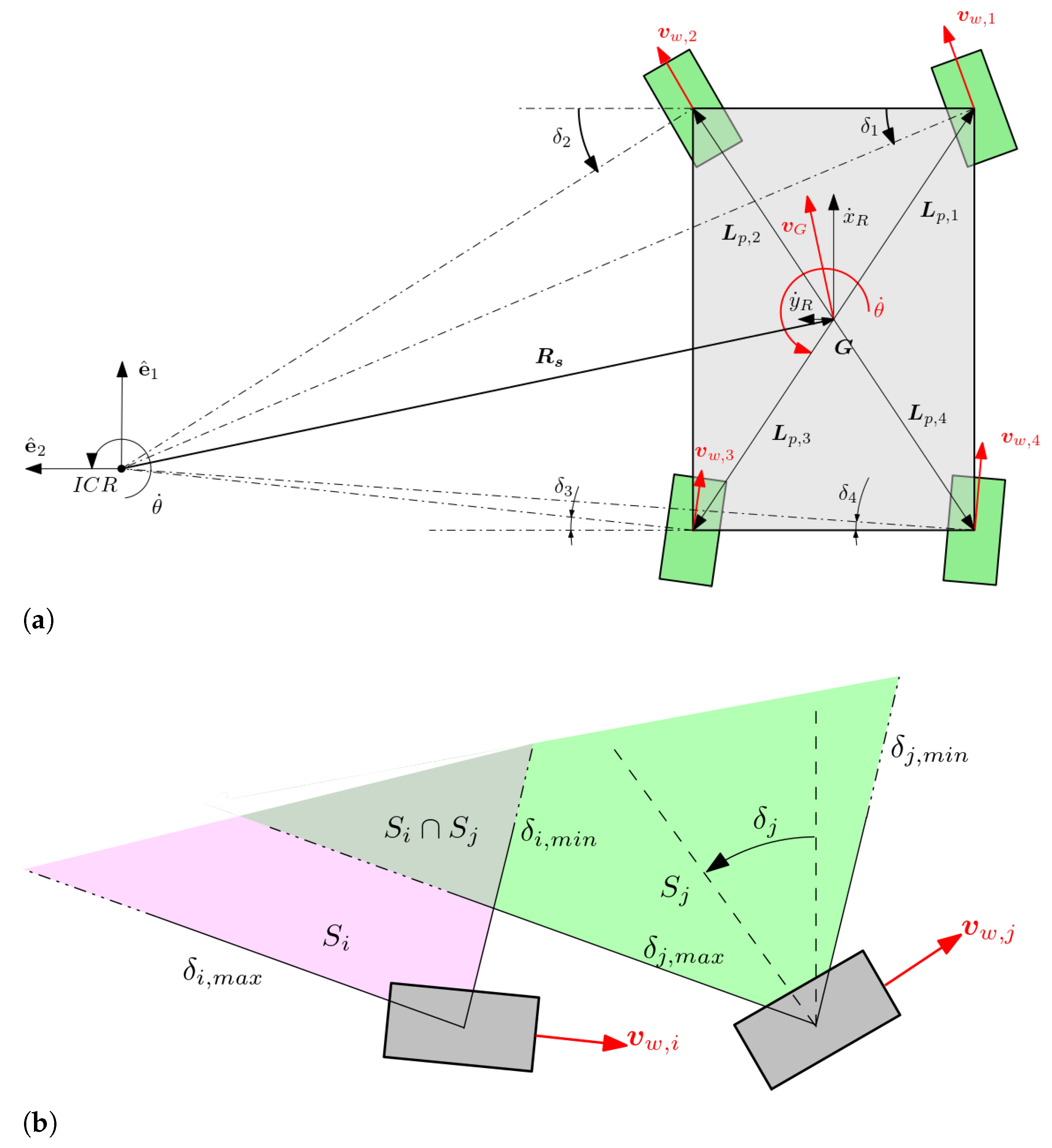
The Archimede planetary rover prototype was first described in detail by Caruso et al. in [27]. This vehicle is a four-wheel steering planetary rover, which possess four articulated legs, formed by complex preloaded modules called S-Structures [24,59], which constitute the vehicle suspension system. Moreover, the rover legs are coupled together by a differential bar. This section aims at providing the description of two models used within the Archimede rover; the first forms the basis for the rover’s wheels odometry system, while the second is used for the rover’s control. It must be noted that for the scope of the development of the models, it had been assumed the pure two-dimensional case. It follows that the articulated legs are considered to be rigid, and the legs are rigidly attached to the body; hence, the lever mechanism has no effect. With reference to Figure 1a, let us introduce a reference frame $(\mathbf{G},{\overline{\mathbf{e}}}_R)$, where ${\overline{\mathbf{e}}}_R=\{\widehat{\mathsf{ı}},\widehat{\mathit{j}},\widehat{\mathit{k}}\}$ is fixed with the chassis of the rover. To the generic wheel of the j-th leg is assigned a new reference frame $({\mathsf{\Gamma }}_{\mathit{j}},{\overline{\mathbf{e}}}_W)$ where ${\overline{\mathbf{e}}}_W=\{{\widehat{\mathbf{e}}}_{\rho },{\widehat{\mathbf{e}}}_{\theta },{\widehat{\mathbf{e}}}_{\varphi }\}$. Consider the planar projection of the body and the wheels as shown in Figure 1a. It is possible to express the linear velocity of the single j-th wheel as follows:

$${\mathit{v}}_{w,j}={\mathit{v}}_{\mathbf{G}}+\dot{\theta }\widehat{\mathit{k}}\times ({\mathsf{\Gamma }}_{\mathit{j}}-\mathbf{G})={\dot{\varphi }}_{w,j}{R}_w{\widehat{\mathit{e}}}_{\rho }$$

(1)

where ${\mathit{v}}_{\mathit{G}}$ and $\dot{\theta }$ are the linear speed vector of the centre of mass of the rover and its angular speed, respectively. Additionally the wheels have a radius $R_w$, while the j-th wheel is characterized by having a driving speed ${\dot{\varphi }}_{w,j}={\dot{\varphi }}_j$ and a steering angle ${\delta }_j$. It is apparent that for every wheel of the system we introduce a vector equation of form Equation (1), which in turn includes two scalar Equations (one for each vector component).

Considering the complete representation of the rover, shown in Figure 1b, and iterating for each wheel the procedure followed to obtain Equation (1), we obtain a matrix relation of the following form:

$${\mathit{A}}_{\mathit{k}}{\dot{\mathit{x}}}_{\mathit{R}}={\mathit{B}}_{\mathit{k}}$$

(2)

where, ${\dot{\mathit{x}}}_{\mathit{R}}\in {\mathbb{R}}^{3\times 1}$ is the vector of the velocity state of the rover body, which is ${\dot{\mathit{x}}}_{\mathit{R}}={[{\dot{x}}_R,{\dot{y}}_R,\dot{\theta }]}^T$. The matrix ${\mathit{A}}_{\mathit{k}}$ is defined as follows:

$${\mathit{A}}_{\mathit{k}}=\left[\begin{array}{ccc}1& 0& -L_{1}sin{\alpha }_1\\ & ⋮& \\ 1& 0& -L_{4}sin{\alpha }_4\\ 0& 1& L_{1}cos{\alpha }_1\\ & ⋮& \\ 0& 1& L_{4}cos{\alpha }_4\end{array}\right]$$

(3)

and the matrix ${\mathit{B}}_{\mathit{k}}$ is:

$${\mathit{B}}_{\mathit{k}}=\left[\begin{array}{c}{R}_1{\dot{\varphi }}_{1}cos{\delta }_1\\ ⋮\\ R_4{\dot{\varphi }}_{4}cos{\delta }_4\\ R_1{\dot{\varphi }}_{1}sin{\delta }_1\\ ⋮\\ R_4{\dot{\varphi }}_{4}sin{\delta }_4\end{array}\right]$$

(4)

${\mathit{A}}_{\mathit{k}}\in {\mathbb{R}}^{8\times 3}$ is a matrix that, under the aforementioned assumptions, is constant in time, and depends only on the geometry of the rover. On the other hand, the matrix ${\mathit{B}}_{\mathit{k}}\in {\mathbb{R}}^{8\times 1}$ contains the wheels’ state parameters, i.e., the wheels’ rotational speed and the steering angles.

The system parameters of the Archimede rover are shown in

Table 1. System parameters for the Archimede rover [27]. Note that the specific configuration of the rover used in the test reported in this work is slightly different in terms of the mass of the rover body compared to that of our previous work.

Component	Value	Unit
Body mass	1.61	kg
Right leg mass	1.58	kg
Left leg mass	1.58	kg
Wheelbase	0.720	m
Track	0.443	m
Height	0.350	m
Wheel diameter (low grousers)	0.170	mm
Wheel diameter (high grousers)	0.186	mm

.

2.1. Odometric System

This paragraph presents the model which the Archimede rover uses and which forms the basis of its wheel odometry system. Recalling the procedure followed in the previous section, it is apparent that Equation (2) represents an over-determined linear system described by eight equations and three variables. However, for this study this system will be directly resolved by using the Moore–Penrose left pseudo-inverse. Hence:

$${\dot{\mathit{x}}}_R={\left({\mathit{A}}_{\mathit{k}}^{\mathit{T}}{\mathit{A}}_{\mathit{k}}\right)}^{-1}{\mathit{A}}_{\mathit{k}}^{\mathit{T}}{\mathit{B}}_{\mathit{k}}$$

(5)

which can be expressed in the inertial frame as follows:

$${\dot{\mathit{x}}}_I={\mathit{R}}^{\mathit{T}}{\dot{\mathit{x}}}_R$$

(6)

where $\mathit{R}$ is the rotation operator in the bi-dimensional case:

$$\mathit{R}=\left[\begin{array}{ccc}cos\theta & sin\theta & 0\\ -sin\theta & cos\theta & 0\\ 0& 0& 1\end{array}\right]$$

(7)

It follows that Equations (5) and (6) are the equations that are at the base of the odometric positioning estimation system, which has been coded and included in the firmware of the Archimede rover prototype, and for the digital twin of the rover in Gazebo and described by a proper C++ plugin. Specifically, the odometric system of the Archimede rover is based on reading at high frequencies the encoders of the eight motors, i.e., both the steering and driving ones. More precisely, by discretizing the time t, it is possible to estimate the rover’s position in the inertial frame at the time frame $t_k$ as follows:

$${\mathit{x}}_I\left(t_k\right)={\mathit{x}}_{I,0}+\sum _{i=0}^k\mathit{R}\left(t_i\right){}^{\mathit{T}}{\dot{\mathit{x}}}_R\left(t_i\right)\Delta t\left(t_i\right)$$

(8)

where ${\mathit{x}}_{I,0}$ represents the initial condition of the rover in the inertial frame, and it is assumed to be non-null in general.

2.2. Steering Control

The control of the rover is based on the well-known concept of the Ackermann steering. More precisely, the inverse differential kinematics of the vehicle is obtained by leveraging this methodology.

2.2.1. General Ackermann Steering

The approach is based on purely geometric concepts and is derived on the basis of two fundamental assumptions: the first is that the vehicle follows a purely rigid motion around a generic “Instantaneous Center of Rotation” (for short ICR), and the second is that the two constraints imposed by the wheels (pure rolling constraint and no lateral slip) are always satisfied at every instant of time during motion. Moreover, we consider that the motion happens on a purely bi-dimensional plane. These considerations and the approach are schematically represented in Figure 2a. It is apparent that by leveraging this approach, by providing high level control signals $({\dot{x}}_R,{\dot{y}}_R,\dot{\theta })$ to the rover, it is always possible to determine an ICR, and then by using geometrical considerations, it is possible to determine exactly at every time instant the variables ${\delta }_i$ and ${\varphi }_i$ of the wheels, $\forall i=1\dots 4$.

2.2.2. ICR Projection Approach

As seen in our previous publication [27] the wheels of the Archimede rover, due to their design, are subjected to both lower and upper constraints for the steering angles, which are summarized in

Table 2. Summary of the Archimede wheel hub’s steering joints lower and upper limitations.

Wheel ID	${\mathit{\delta }}_{\mathbf{min}}$	${\mathit{\delta }}_{\mathbf{max}}$
1	$-33.7$${}^{\circ }$	$+93.0$${}^{\circ }$
2	$-93.0$${}^{\circ }$	$+33.7$${}^{\circ }$
3	$-33.7$${}^{\circ }$	$+93.0$${}^{\circ }$
4	$-93.0$${}^{\circ }$	$+33.7$${}^{\circ }$

. As will be shown in this section, by leveraging the general Ackermann steering formulation and by applying a technique we call the “ICR projection” approach, it is possible to account for those constraints elegantly. Specifically, by denoting the general ICR point with ${\mathrm{\Omega }}_r=\left[x_{ICR},y_{ICR}\right]$, under the Ackermann conditions the ICR must lie on the driving axis of the generic wheel i. With reference to Figure 2b, by sweeping the driving axis from ${\delta }_{i,min}$ to ${\delta }_{i,max}$, it is possible to determine a region of all admissible locations for the ICR for the wheel i, which we will call $S_i$. By introducing a new wheel j, it is possible to determine a new region $S_j$. It is apparent that ${\mathrm{\Omega }}_r$ must lie in a subregion which is obtained as the intersection of the single ones, i.e., $S=S_i\cap S_j$. Performing the process that was described for generic wheel i, and iterating it for each wheel of the rover yields a set of regions where ${\mathrm{\Omega }}_r$ is allowable for each wheel, and thus, for the entire system. It can be demonstrated that the surfaces that have been obtained are five in number, and they are all disconnected from each other, and can be seen as the black regions from Figure 3. We will denote from now on the set of admissible regions of ${\mathrm{\Omega }}_r$ as $S^{+}$, and the set of ineligible regions as $S^{-}={\mathbb{R}}^2$\$S^{+}$. It is, therefore, necessary to develop an approach that makes sure that regardless of the velocity high level control signals commanded to the rover, ${\mathrm{\Omega }}_r$ always falls within $S^{+}$. For this purpose, a method is introduced that is based on projecting the ICR into the admissible zones. Specifically given a general control signal command, a ${\mathrm{\Omega }}_r$ point is obtained; subsequently, a new ICR point ${\mathrm{\Omega }}_r^{*}$ defined as follows is then calculated:

$$\begin{array}{c}\hfill {\mathrm{\Omega }}_r^{*}=\left\{\begin{array}{cc}{\mathrm{\Omega }}_r,\hfill & \mathrm{if}{\mathrm{\Omega }}_r\in S^{+}\hfill \\ {\mathit{P}}_{pr},\hfill & \mathrm{if}{\mathrm{\Omega }}_r\in S^{-}\wedge {\mathit{P}}_{pr}\in S^{+}\wedge \left|\right|{\mathit{P}}_{pr}-{\mathrm{\Omega }}_r{\left|\right|}_{min}\hfill \end{array}\right.\end{array}$$

(9)

Note that this method is entirely compatible with non-symmetric steering capabilities, i.e., when the wheels have diverse steering capabilities. Indeed, since the model itself depends on the notion that the ICR ${\mathrm{\Omega }}_r$ must always be inside an eligible region $S^{+}$, and that this in turn is the intersection of each wheel subregion $S_i$, as long as it is possible to determine $S_i$ for each i-th wheel, the model works fine. Along the same lines, the model supports non-steerable wheels as well—in this case, $S_i$ for the non-steerable wheel becomes a line—and to vehicles with an arbitrary number of wheels. For example, the MSL rover “Curiosity” has six wheels, of which only the front and rear wheels are steerable, with the middle pair fixed; the model in this case would consider $S^{+}$ as a line coincident with the axis of the middle wheels.

2.2.3. Drive Modes

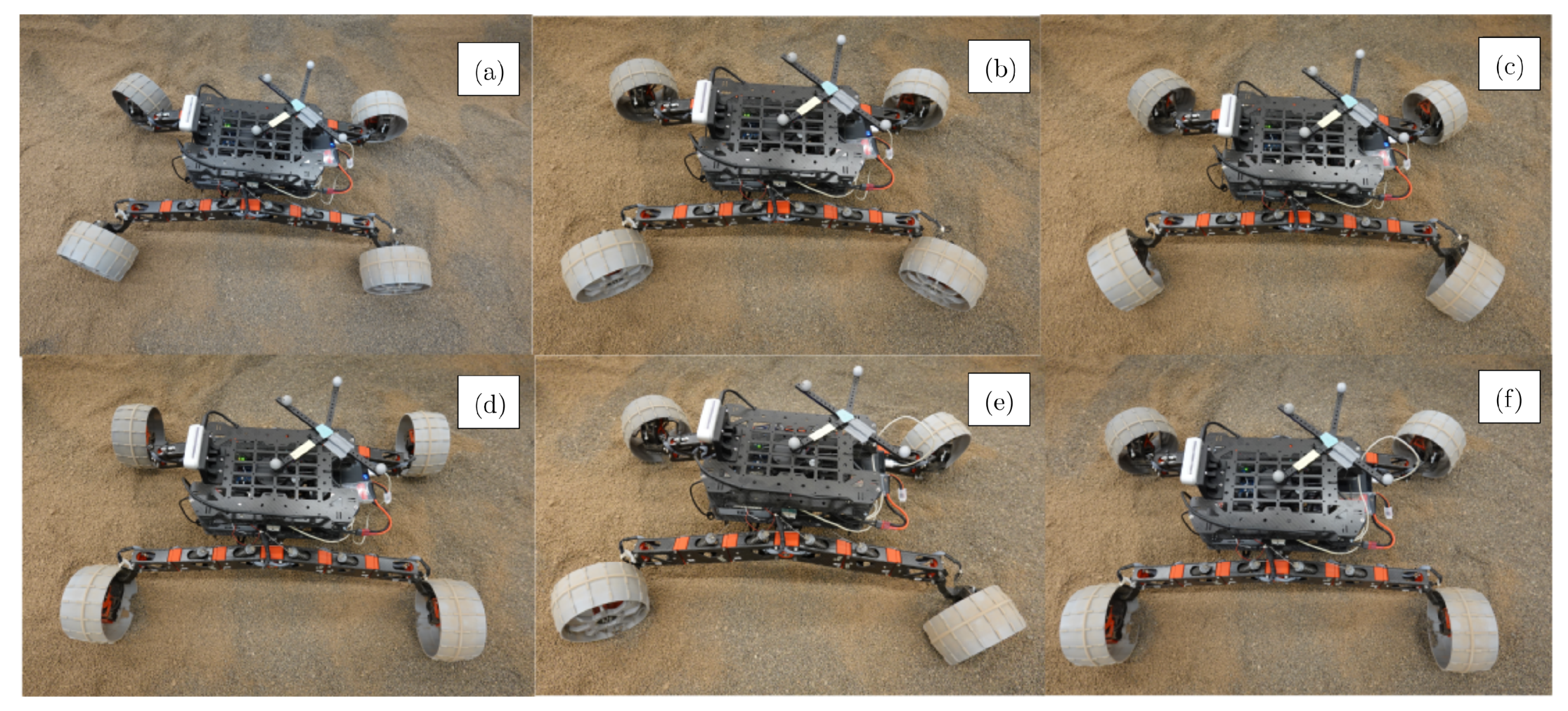
With the help of Figure 3, and more precisely considering different subsets of $S^{+}$, it was possible to identify some characteristic driving modes, which are interesting for a general four-wheel steering vehicle which is subjected to steer joints constraints, such as the Archimede rover in this instance. The modes identified can be listed as follows:

• Car-Like mode: the steering joints of the rear wheels are locked, and hence, the rover ICR is constrained to pose along the driving axis of the rear wheels of the rover. In this configuration, only the front wheels are allowed to steer, the same as regular cars.
• Symmetric Ackermann mode: Very similar to the previous mode, differing from it only because in this specific driving mode the ICR of the rover is constrained to be along a line passing through the origin of the rover and coincident with its $\widehat{\mathit{j}}$-axis.
• In-Place rotation: The ICR is unique and coincides with the center of the rover. In this driving mode, the rover is characterized by not having any linear speed, while the wheels are arranged in such a configuration that allow the rover to rotate on the spot. This derives from the Symmetric Ackermann mode.
• Lateral Drive mode: The ICR formally does not exist. In practice, it is located somewhere along the $\widehat{\mathsf{ı}}$ axis of the rover frame and infinitely away from it. It follows that the wheels are turned by 90° around their steering axis, thus allowing the rover to move sideways.
• Parallel Drive mode: As in the previous case, the ICR formally does not exist. The wheels are characterized by the fact that they turn with the same steering angle $\gamma$, thus allowing the robot to move in a parallel way. The rover possesses only components of linear velocities, but not angular velocity.
• Outer Ackermann mode: With reference to Figure 3, this driving mode has been derived by considering in the set of the admissible ICR surfaces $S^{+}$ only the two large ones placed on the side of the rover. It is apparent that the two cases of the Car-Like and Symmetric Ackermann are particular cases of this bigger driving mode case.
• Inner Ackermann mode: This drive mode has been derived by considering in the set of ICR $S^{+}$ eligibility surfaces only the central surface located under the belly of the rover, which is visible in Figure 3. It is apparent that the In Place rotation mode is a degenerate case of this bigger driving mode case.
• General Ackermann mode: This driving mode has been obtained by combining the previous modes, i.e., by considering every surface belonging to $S^{+}$.

Finally, some of the aforementioned identified driving modes can be better seen in Figure 4.

Recalling the example of the MSL rover described in the previous section, the specific wheels arrangement of the vehicle would only allow Symmetric Ackermann.

2.2.4. Controller Architecture

In order to implement the functionality described up to this point, the system takes advantage of several control modules. In particular, it is important to distinguish the high-level controller from the low-level motor control system. Indeed, while the former takes care of the kinematics of the rover, pose estimation, path planning, and navigation, the latter accepts simple control inputs (${\delta }_j$ and ${\dot{\varphi }}_{w,j}$) provided by the ICR planner and regulates the single motors that actuate the steering and rotation of the wheels. The steering actuation in particular is carried out via PID controller with a feed-forward module; the wheels are actuated using a simpler PI controller. Both are equipped with saturation blocks and anti-windup. A high-level diagram of the overall controller architecture is shown in Figure 5.

3. Comparison—Study Preparation

This section aims to comprehensively describe the preparation followed in order to conduct this study. Specifically, the experimental test modes, how they will be conducted, and what of the individual modes is to be studied will be described first. Next, the setup of the simulation environment is described and used as a tool to make a comparison with the experimental results about the accuracy of the rover positioning system. Finally, two different experimental testbeds in which the experiments were conducted will be described, according to the test modes described in the first paragraph.

3.1. Test Modes

In this paragraph, the two main test modes are described that have been chosen for the Archimede rover. More precisely, for each of the test modes the experimental tests have been performed along different paths, in different driving modes for the rover and with different mean speed $\omega$ of the rover wheels. The purpose of each individual test mode is to evaluate and study a certain characteristic of the rover. The two main test modes can be classified as follows.

3.1.1. Driving on Flat Terrain

For this test mode the experimental sandbox was prepared such that it mimics an horizontal surface, as close as possible. Additionally, in this test mode, the Archimede rover was driven with the Symmetric Ackermann, lateral and parallel modes, along six different path shapes: straight, lateral, diagonal line, circle, S-path, and square. Finally, these drive tests had been conducted with four different levels of commanded mean speed to the wheels, which are $1.2$ $\mathrm{red} {\mathrm{s}}^{-1}$ (we label it ${\omega }_1$), $2.4$  $\mathrm{red} {\mathrm{s}}^{-1}$ (labeled ${\omega }_2$), $3.6$  $\mathrm{red} {\mathrm{s}}^{-1}$, and $4.8$  $\mathrm{red} {\mathrm{s}}^{-1}$. What we aim to evaluate with this type of test mode is to assess the goodness of the rover’s positioning system in space, and that it is moving on highly non-ideal ground and far from the assumptions used for numerical model development. For this purpose, the same tests performed experimentally are repeated in the simulation environment, described below, also in order to evaluate the reality gap.

3.1.2. Driving on an Inclined Plane

For this test mode, the Archimede rover was driven along a slope of the sandbox that was progressively increased by 5$°$ each time up to 20$°$, namely the maximum value for the slope allowed. We conducted some experimental tests with this test mode in order to study and evaluate the traction capabilities and the ability of the rover to climb steep slopes. Finally, for every value of the slope, drive tests were performed using three of the rover’s driving modes such as straight, lateral, and parallel, and all of them with two mean speeds commanded to the wheels, namely ${\omega }_1$ and ${\omega }_2$.

As it will be outlined in Section 3.3, the two aforementioned experimental test modes have been repeated over two different Experimental testbed setups, in which we have basically changed the soil within the sandbox as well as the shape and characteristics of the wheels. This had been done in order to provide a first understanding of the influence of the wheel shape on the rover performances, while driving on a specific soil.

3.2. Simulation Framework Setup

This paragraph briefly describes the simulation framework for the Archimede rover that had been set up and used to compare the results obtained for the Drive on horizontal surface mode. Specifically, the simulation framework that has been built is based on the use of Robot Operating System (ROS) [64] middleware and the multibody simulation software package Gazebo [65], therefore allowing co-simulation through the known ROS-Gazebo bridge. Specifically, a series of ROS packages was developed, each providing different core functionalities, which together have the role to take care of setting up and conducting the dynamic simulations of the Archimede rover in Gazebo, and also to mimic as close as possible the systems and the functionalities of the real-world rover. One package is responsible for the modeling of the Archimede rover. The rover and its mechanisms were modeled by leveraging the ROS package xacro. This package allows for parametric modeling and the definitions of the so-called “macros”. The modeling is completed by defining some links in appropriate files (.xacro), and then by connecting them through appropriate joints, recorded in the same .xacro file. A short example of the modeling within .xacro files can be seen in the listings in Listing 1.

Listing 1. Short example of the modeling in xacro/URDF robot description files. Here, the code is the structure of a xacro macro that describes a two-link one-joints kinematic chain composed of link_1 and link_2 connected through joint joint_1.

It must be pointed out that in this simulation framework, we have assumed that the S-Structures, comprising the rover’s legs articulations, are rigid enough to consider the leg as a single body. This assumption is based on the fact that the velocities we deal with in this specific series of tests are comparatively low for the rover (≤0.34 m ${\mathrm{s}}^{-1}$), and thus, the legs never show any deflection caused either by the dynamics of the rover or by accidental contacts with obstacles. Indeed, the test terrains are free from objects larger than a few millimeters that could impact on the wheels.

On the other hand, appropriate closed chains have been defined in the description file of the rover in order to develop the differential mechanism between the bogies of the rover, which is described in detail in [27]. Finally, this package contains the definition of which C++ plugin to load within the Gazebo simulation environment. The plugins have the role to mimic and simulate every system present on the experimental prototype. It follows that the model of the rover contains plugins that simulate the IMU sensor, the 2D Lidar range sensor, the wheels encoders, the RealSense D435i stereo-camera, the kinematics, the actuation of the joints, and finally the wheels odometry subsystem implementing the model described in the previous section. Other packages instead have the role of implementing the rover kinematics applying the earlier described ICR projection approach, telecommand, visualization features, mapping, SLAM, the navigation stack, and so on. A graphical representation of the final rover model in the Gazebo simulation environment is shown in Figure 6. From the same figure, the simulation environment containing random obstacles can be seen, as well as the model of the Archimede rover, the rays of the 2D Lidar scanner, and the field of view of the RealSense stereo camera.

The physics engine used in Gazebo is the well-known ODE (Open Dynamics Engine). Contacts are only allowed in between the wheels and the terrain and follow a multi-point penalty-based approach, where stiffness, damping, and friction properties are set accordingly.

3.3. Experimental Testbed Setup

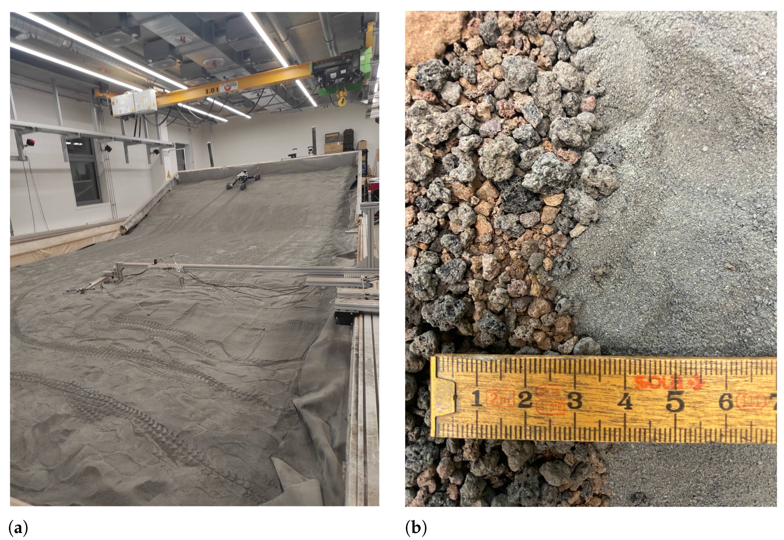
The experiments have been conducted with the Archimede rover prototype in the sandbox of the Planetary Exploration Laboratory (PEL) of DLR’s Institute of Robotics and Mechatronics, located in Oberpfaffenhofen, Germany. Moreover, for every experimental test that had been conducted in the PEL, the Archimede rover had been tracked by an ART DTRACK optical tracking system, which reconstructed the rover motion. In the PEL it is possible to tilt a portion of the sandbox, thus allowing to evaluate the rover capability to climb steep slopes. Figure 7a shows the experimental setup of the DLR PEL sandbox, the tracking system, the tilting side of the sandbox, and the Archimede rover driving on a 20$°$ slope.

Two different test setups were explored during the rover experiments. This had been done in order to evaluate the effect of the design of the wheels while driving over different ground substrates. Specifically, the two test setups are:

Test Setup A

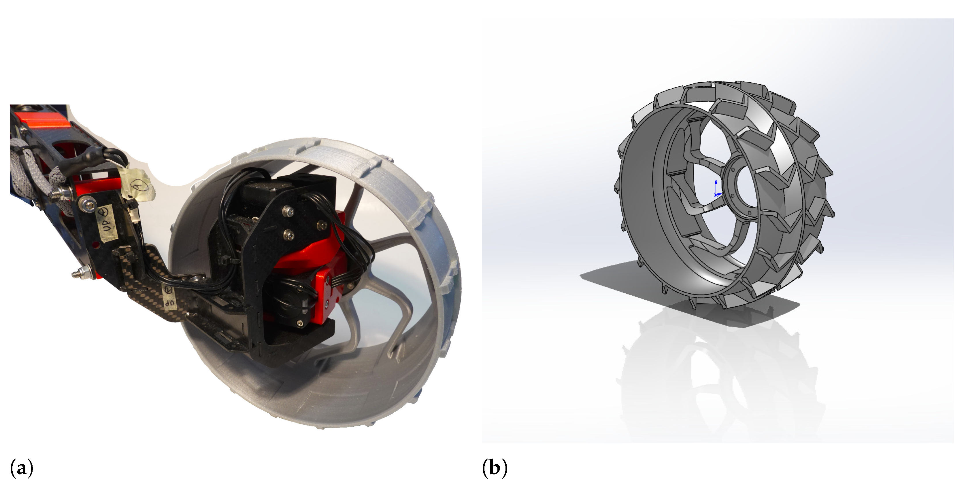
The sandbox of the PEL had been filled with granular lava having grain sizes in between 1 $\mathrm{m}$$\mathrm{m}$ and 5 $\mathrm{m}$$\mathrm{m}$ and the Archimede rover has been equipped with a set of wheels with low grousers, which can be seen from Figure 8a.

Test Setup B

The sandbox of the PEL had been filled with the lunar regolith simulant EAC-1A [66], a very loose soft soil with submillimeter granularity. In this case, the Archimede rover has been equipped with a set of wheels with high grousers, which can be seen from Figure 8b.

The two types of soil are shown and compared in Figure 7b. In the figure, the grain size is shown of the two kind of soils, which are compared to a scale. For both test setups, A and B, the test modes 1 and 2 were performed, namely the Drive on flat terrain and the Drive on inclined plane.

4. Results and Discussion

This section reports and discusses in detail the most significant results that were obtained during the experiments done with the Archimede rover. The results obtained for horizontal terrain are presented and discussed first, followed by the results for driving on inclined terrain.

4.1. Results for the Test Case of Driving on a Flat Terrain

In this subsection, we report the results that have been obtained for the test mode corresponding to driving on flat terrain. The aim of these results is to evaluate the goodness of space robot positioning estimation system by using only the wheels odometry technique, which is based on the model outlined in Section 2.1 and implemented in the firmware of the Archimede rover.

Specifically, what is intended to be shown in this section is a demonstration of the goodness-of-fit of the odometry-based rover placement estimation system in a highly non-ideal environment. In fact, all the assumptions made in the model development phase are violated as soon as the rover is driven over granular terrain. We want to evaluate this in a qualitative but not quantitative manner, and hence, we perform a statistical analysis over a large set of experiments, and for purely demonstrative purposes, whether it is possible to use such a system in a highly non-ideal environment, quantify its accuracy, and go on to evaluate its deviation from the real and ideal case, recreated in the simulation environment.

For the tests performed for the Archimede rover odometry subsystem demonstration, we evaluated it both experimentally and numerically, in the appropriate Gazebo simulation environment, outlined in the previous section. For the experimental evaluation of the system, the surface of the sandbox has been leveled as accurately as possible. In order to compare the results, the tests carried out experimentally were reproduced under the same conditions in the simulated environment.

Since the purpose is purely demonstrative, it was decided to take four different types of paths as examples: (i) a 20$°$ diagonal line; (ii) a path drawing a quarter of a circle; (iii) a path drawing an “S-like” shape; (iv) a path drawing a square shape. The findings of these tests are reported in Figure 9. It is important to point out that the set of selected trajectories, used for this demonstrative purpose, refers to the Test Setup A. The figure depicts, for all the four trajectories taken as demonstrative examples, the evolution of the real trajectory of the rover in experiments and simulation (tracking (experimental)), and (tracking (gazebo), respectively) and the trajectory reconstructed by the odometry subsystem in experiments and simulation (odometry (experimental) and odometry (gazebo), respectively); all were compared to the nominal trajectory the rover.

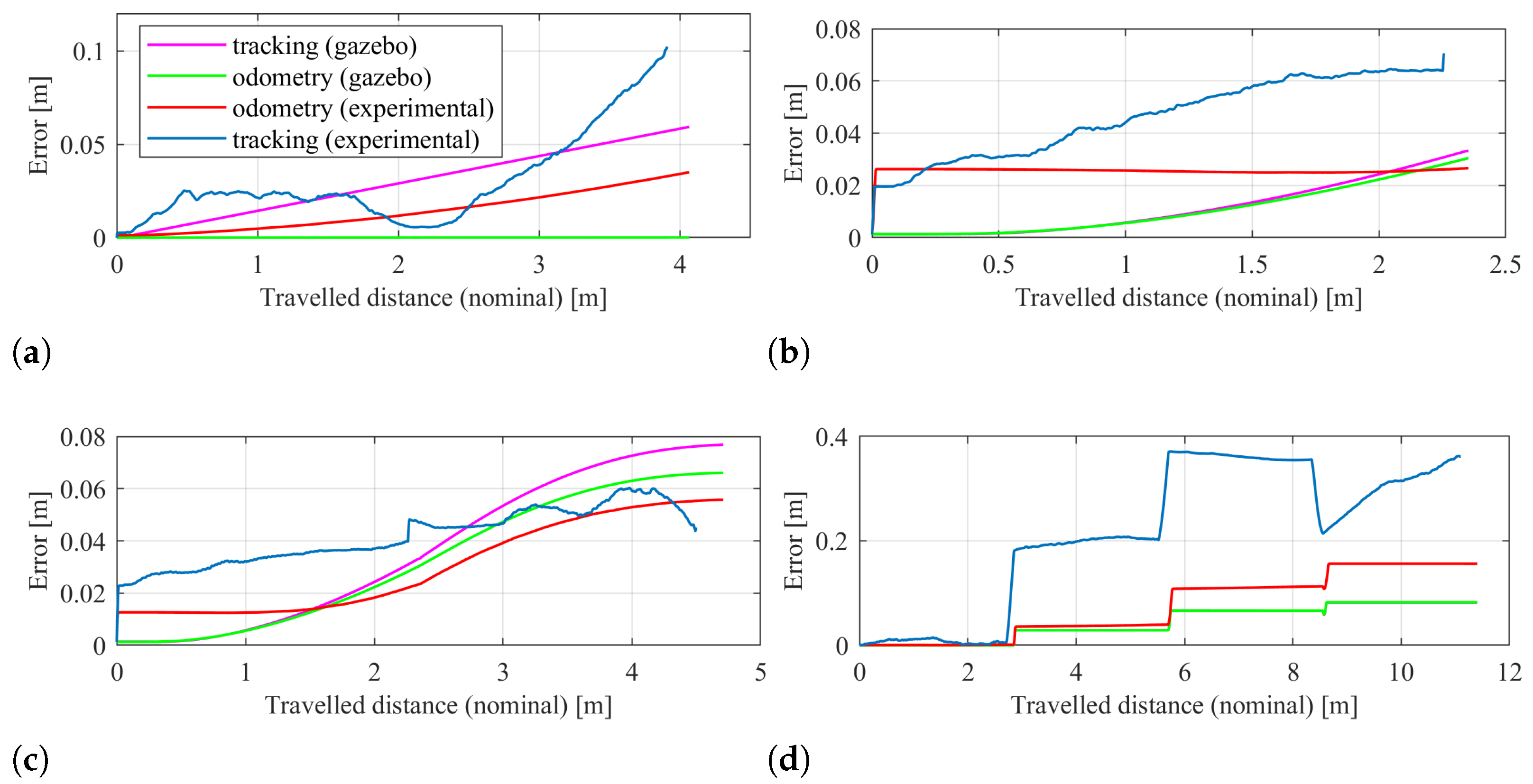
From Figure 9, we can clearly see that the shape of the imposed path is preserved in all cases, and the curves are relatively close to each other. However, they are all subjected to many different source of inaccuracies, and the curve that shows greater deviation is, as predicted, the one corresponding to the tracking experiment. The error estimation evolution of all trajectories, for the four different selected paths, compared to the nominal trajectories, can be seen in Figure 10. Sources of inaccuracies can be linked to the fact that the soil is loose and granular, which subjects the rover’s wheels to longitudinal and lateral slippage. Additionally, the surface has minor bumps and craters, and the experimental tests are distinguished by additionally involving a vertical displacement of the rover. This is evident from Figure 11a, which depicts the rover’s vertical displacement in the scenario of the square path. The disparity between the effective radius of the wheel and the nominal radius of the wheel, as well as the sinkage phenomena, are additional sources of inaccuracy. Another cause of error is the time it takes for commands to be sent and received via the ROS network. Numerical errors also contribute to this, i.e., the one introduced by the time integration scheme or the truncation error caused by the least-square method used to compute the odometric step. Inertial effects acting on the rover might be another cause of errors. Last but not least, since odometric position estimate relies on dead reckoning, it follows that errors tend to compound with time, becoming more noticeable as the traveled distance rises.

It might be worth noting that, while the simulated trajectories (both the actual trajectory in Gazebo and its odometry estimate, and also the odometry in the experimental setup) show good adherence to the nominal path, the experimental tracking shows considerable deviation. This can be split into two different problems:

• Gazebo simulations. The sources of error in this case are essentially related to the dynamics of the system and the interaction with the ground, which is modeled as a planar hard surface with friction. The effect these aspect have on the trajectory appear somewhat negligible.
• Experimental odometry. In this case, the sources of error are many and more diverse, primarily: terrain yield, slip, non-planar terrain, and non-uniform soil. We can, thus, expect that the rover drifts more substantially from the intended path. Experimental results show this quite clearly.

Figure 11b shows in the form of a bar plot the end-point trajectory relative position error, for all the selected paths, evaluated between the real and estimated pose of the rover for the two cases: experimental and simulated in Gazebo.

Both the experimental and numerical tests exhibit an error of less than 10%. Furthermore, it is clear that the errors of the experimental paths are larger than those detected in numerical models. This is because the experimental scenario has many more causes of error, where the terrain’s unpredictability and unsuitability are the first of them.

In the instance of the numerical simulations, the diagonal path is the one that exhibits a greater end-point position error. This can be explained by the fact that all the wheels spin right away at the start of the simulation to get to the commanded steer set-point, producing an inertial effect that causes the rover to spin in the opposite direction. This causes the rover to have a non-null heading angle with respect to nominal at the beginning of the simulation, causing it to deviate from the nominal path. This effect has not been detected in the experimental tests, probably because it is marginal with respect to the other sources of error (e.g., terrain yield, slip).

4.2. Results for the Test Case of Driving on Inclined Plane—Slip Evaluation

The final paragraph of this section presents and discusses in detail the most significant results that were obtained for the case of driving on sloping terrain. It is important to specify that, unlike the previous section, both test setups were analyzed. In addition, a more quantitative analysis is conducted in this section than in the previous one. For this purpose, it has been elected for all the drive tests to compute statistical features, such as mean, standard deviation, and median, regarding the slip s the wheels undergoes. The analysis of this feature helps understanding the performances and the traction capabilities of the Archimede rover, as the wheel shape changes and the nature of the terrain on which they travel. As a final note, we would like to report that all results presented in this section refer to experimental tests. No numerical simulations were performed for this test mode.

In Figure 12, the median evolution of the slip is reported, which is computed by grouping all the tests performed for each level of the sandbox slope, and clustered by the mean commanded angular speeds to the wheels, namely ${\omega }_1$ and ${\omega }_2$. The slope of the sandbox has been labeled with $\sigma$. Specifically, Figure 12a shows the evolution of the median of the slip s for the case of Test Setup A, while Figure 12b shows the same for the case of Test Setup B. The first phenomenon that can be seen from these graphs is that by increasing the slope, the slip the wheels are subjected to tends to increase with an exponential trend. However, we can see that the median slip evolution for the Test Setup B is characterized by a lower gradient, and in general lowers slip values, with respect the Test Setup A. Suggesting that the shape of the wheel is better suited for the type of soil used in Test Setup B, and grants more traction over that kind of terrain. A fascinating result that can be seen from these graphs regards the influence that the mean speed of the wheels have on the wheels slip. In particular we can see from both figures that the mean speed of the wheels does have a not negligible influence on the slip experienced by the rover. However, we can see that the influence of the speed have opposite effects for the two test setups. More precisely, for the Test Setup A, we can see that by increasing the mean speed of the wheels also the slip experienced by the rover increase; however, for the Test Setup B, we can observe the opposite trend, i.e., by increasing the mean speed, the slip tends to decrease. In our opinion, this is due to the nature of the soil, which for this test setup is extremely fine and comparable to a fluid. Specifically, we believe that for low speeds the effects of the soil, such as sinkage and so on, are prevalent. When the speed increases, a higher flow rate of the soil is observed, thus allowing for the wheel to exert more traction capabilities on that kind of soil. Finally, with reference to the same figure, we can see that for the tests conducted at sandbox’s slope of 0$°$ the median of the slip the wheels are subjected assume comparable values, and remains very low. In fact, we can observe a median of the slip around 5%.

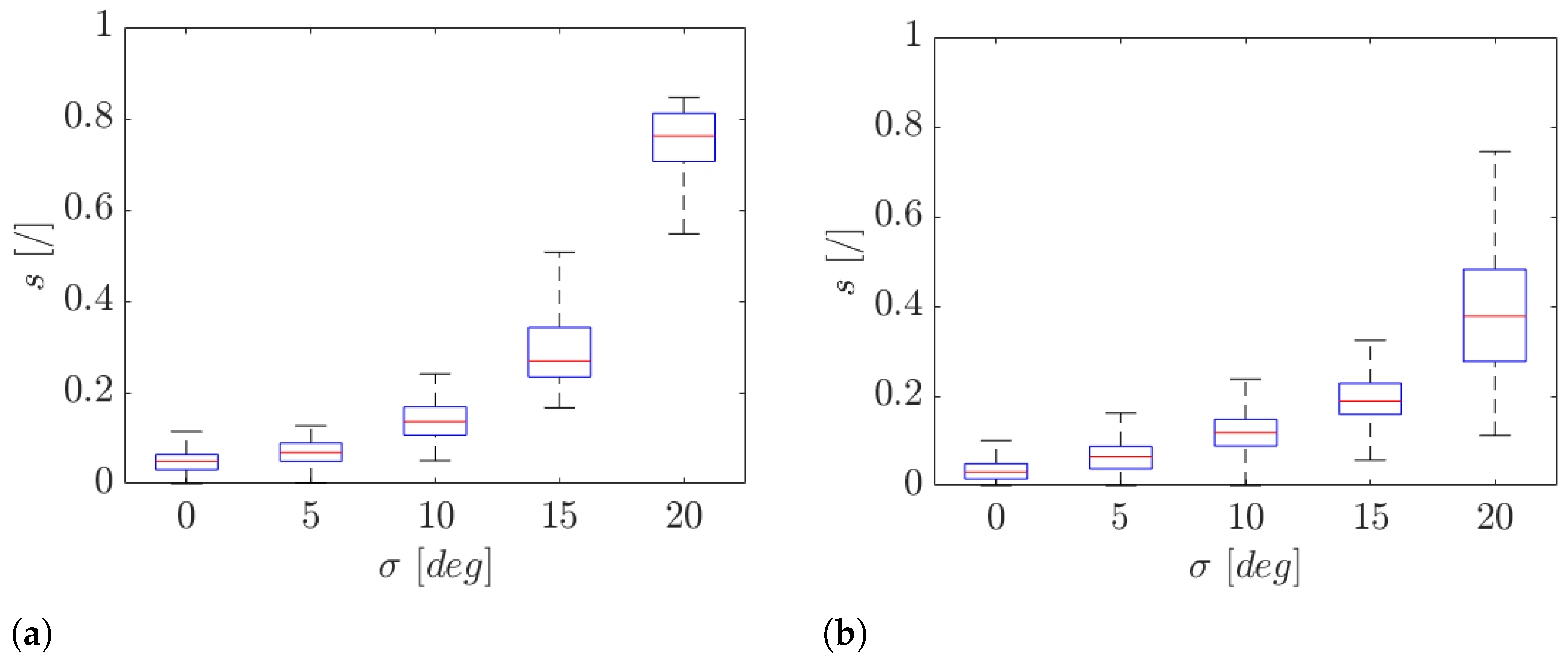
Figure 13, the statistical evolution of the slip is reported, shown in form of box plots, as a function of the slope angle of the sandbox. The results are grouped together without classifying the tests based on the mean speed of the rover’s wheels. This type of analysis gives information on the expected slip ratio for trajectories where velocity is not directly commanded or known in advance or where there are multiple velocities involved, e.g., when frequent stops are foreseen.

A statistically significant difference can be seen between the two test setups. The boxes in the two cases do not overlap. It is also noted how the interquartile range tends to increase and is more visible as the slope increases, suggesting greater variability of the measures. Especially the variability of the measures is very pronounced for the last slope level for the Test Setup B case. Finally, one last thing that can be observed is that all the boxes in the figure show a clear symmetry with respect to the relative median, suggesting a Gaussian distribution of the measurements taken, thus providing information about their goodness-of-fit.

Figure 14 shows the box plots that have been obtained considering the ratio of slip s, grouped with respect to the mean velocities of the wheels ${\omega }_1$ and ${\omega }_2$, for the two test setups and considered individually for each different level of sandbox’s slope $\sigma$. This figure shows results that highlights the influence of the mean speed of the wheels on slip observed. Specifically, the top row refers to the tests conducted in the context of Test Setup A, while the bottom row refers to ones conducted in the context of Test Setup B. Moreover, the columns, starting from the left to the right refer to the slopes $\sigma$ of 5, 10, 15, and 20 degrees, respectively. As seen from Figure 12, we can observe a general trend for the slip to increase exponentially with the slope, and Test Setup B shows lower values of the median of the slip compared to Test Setup A. We can also see from this figure that the mean speed of the wheels, between the two test setups, have an opposite influence on the slip observed. Again, it can be seen that the experiments for the Test Setup B exhibit a clear symmetry with respect to the median, leading the measurements back to a Gaussian distribution. In fact, there is a statistically significant difference with respect to $\omega$, especially at high slopes. On the other hand, the experiments related to Test Setup A lose the symmetry property, indicating distributions that are clearly not normal. This suggests an insufficient number of experiments to show a statistically significant difference, whereas we would have expected it with a congruent number of valid experiments.

5. Conclusions

This paper presents the development of a two-dimensional model, based on certain simplifying assumptions, as the foundation and starting point for a positioning estimation system for a four-wheel steering rover. It also introduces a model that utilizes the well-known concept of Ackermann steering for rover control and implements the innovative concept of ICR projection. The aim is to ensure adherence to steering joint limits and the continuous validity of Ackermann steering conditions. The accuracy of the odometry subsystem is assessed through simulation and experimental testing, specifically focusing on driving the rover on a flat surface. The simulation results demonstrate the system’s ability to accurately estimate the rover’s planar position with an error rate of less than 5%. However, during real sandbox experiments, the system exhibits reduced accuracy due to various sources of inaccuracy. Nevertheless, for sufficiently short trajectories, this system can still provide a reasonably accurate estimate of the rover’s planar position, as indicated by the results showing an error rate of less than 10%. These findings confirm that an accurate position estimate for this type of system is achieved by combining and merging other methodologies, rather than relying solely on wheel encoder-based odometry. Finally, it is observed that the appropriate design of the rover wheels, grousers, and other mechanical characteristics is crucial in ensuring high performance and traction capability over different terrains, depending on their type, nature, and mechanical characteristics.

Future works will see the development of a heuristics-based model for soft soils that can be implemented in common dynamics simulation software. This, compared to more realistic soil models [30,36], will be considerably more lightweight and will enable simulation over large distances. A variation of said models will be implemented in the odometry of the rover, allowing for more precise position determination.

References

1. Caruso, M.; Scalera, L.; Gallina, P.; Seriani, S. Dynamic modeling and simulation of a robotic lander based on variable radius drums. Appl. Sci. 2020, 10, 8862. [Google Scholar] [CrossRef]
2. Liu, Y.; Li, X.; Wang, P.; Zhang, X.; Zhu, H.; Cai, G. Multi-Objective, Multi-Disciplinary Design Optimization and Multi-Attribute Evaluation of Hybrid Rocket Motors Used for Manned Lunar Lander. Aerospace 2023, 10, 272. [Google Scholar] [CrossRef]
3. Grotzinger, J.; Crisp, J.; Vasavada, A.; Anderson, R.; Baker, C.; Barry, R.; Blake, D.; Conrad, P.; Edgett, K.; Ferdowski, B.; et al. Mars Science Laboratory mission and science investigation. Space Sci. Rev. 2012, 170, 5–56. [Google Scholar] [CrossRef]
4. Muirhead, B.; Karp, A. Mars Sample Return Lander Mission Concepts. In Proceedings of the IEEE Aerospace Conference Proceedings, Big Sky, MT, USA, 2–9 March 2019; Volume 2019. [Google Scholar]
5. Campagnola, S.; Yam, C.; Tsuda, Y.; Naoko, O.; Kawakatsu, Y. Mission analysis for the Martian Moons Explorer (MMX) mission. Acta Astronaut. 2018, 146, 409–417. [Google Scholar] [CrossRef]
6. Newman, C.E.; Hueso, R.; Lemmon, M.T.; Munguira, A.; Vicente-Retortillo, Á.; Apestigue, V.; Martínez, G.M.; Toledo, D.; Sullivan, R.; Herkenhoff, K.E.; et al. The dynamic atmospheric and aeolian environment of Jezero crater, Mars. Sci. Adv. 2022, 8, eabn3783. [Google Scholar] [CrossRef] [PubMed]
7. Mahaffy, P.; Webster, C.; Cabane, M.; Conrad, P.; Coll, P.; Atreya, S.; Arvey, R.; Barciniak, M.; Benna, M.; Bleacher, L.; et al. The sample analysis at mars investigation and instrument suite. Space Sci. Rev. 2012, 170, 401–478. [Google Scholar] [CrossRef]
8. Webster, C.; Mahaffy, P.; Atreya, S.; Moores, J.; Flesch, G.; Malespin, C.; McKay, C.; Martinez, G.; Smith, C.; Martin-Torres, J.; et al. Background levels of methane in Mars’ atmosphere show strong seasonal variations. Science 2018, 360, 1093–1096. [Google Scholar] [CrossRef]
9. Lapotre, M.; Ewing, R.; Lamb, M.; Fischer, W.; Grotzinger, J.; Rubin, D.; Lewis, K.; Ballard, M.; Day, M.; Gupta, S.; et al. Large wind ripples on Mars: A record of atmospheric evolution. Science 2016, 353, 55–58. [Google Scholar] [CrossRef]
10. Schuster, M.; Muller, M.; Brunner, S.; Lehner, H.; Lehner, P.; Sakagami, R.; Domel, A.; Meyer, L.; Vodermayer, B.; Giubilato, R.; et al. The ARCHES Space-Analogue Demonstration Mission: Towards Heterogeneous Teams of Autonomous Robots for Collaborative Scientific Sampling in Planetary Exploration. IEEE Robot. Autom. Lett. 2020, 5, 5315–5322. [Google Scholar] [CrossRef]
11. Wedler, A.; Schuster, M.; Müller, M.; Vodermayer, B.; Meyer, L.; Giubilato, R.; Vayugundla, M.; Smisek, M.; Dömel, A.; Steidle, F.; et al. German Aerospace Center’s advanced robotic technology for future lunar scientific missions: DLR’s Advanced Robotic Technology. Philos. Trans. R. Soc. A Math. Phys. Eng. Sci. 2021, 379, 20190574. [Google Scholar] [CrossRef]
12. Sheppard, R.Y.; Thorpe, M.T.; Fraeman, A.A.; Fox, V.K.; Milliken, R.E. Merging Perspectives on Secondary Minerals on Mars: A Review of Ancient Water-Rock Interactions in Gale Crater Inferred from Orbital and In-Situ Observations. Minerals 2021, 11, 986. [Google Scholar] [CrossRef]
13. Mallapaty, S. China has landed its first rover on Mars—Here is what happens next. Nature 2021, 593, 323–324. [Google Scholar] [CrossRef] [PubMed]
14. Muirhead, B.; Nicholas, A.; Umland, J.; Sutherland, O.; Vijendran, S. Mars Sample Return Campaign Concept Status. Acta Astronaut. 2020, 176, 131–138. [Google Scholar] [CrossRef]
15. Witte, L.; Heffels, A.; Killian, M.; Knapmeyer, M.; Lange, C.; Toth, N.; Tsakyridis, G.; Wedler, A. A robotically deployable lunar surface science station and its validation in a Moon-analogue environment. Planet. Space Sci. 2020, 193, 105080. [Google Scholar] [CrossRef]
16. Tsuda, Y.; Saiki, T.; Terui, F.; Nakazawa, S.; Yoshikawa, M.; Watanabe, S.I.; Team, H.P. Hayabusa2 mission status: Landing, roving and cratering on asteroid Ryugu. Acta Astronaut. 2020, 171, 42–54. [Google Scholar] [CrossRef]
17. Schuster, M.; Brunner, S.; Bussmann, K.; Büttner, S.; Dömel, A.; Hellerer, M.; Lehner, H.; Lehner, P.; Porges, O.; Reill, J.; et al. Towards Autonomous Planetary Exploration: The Lightweight Rover Unit (LRU), its Success in the SpaceBotCamp Challenge, and Beyond. J. Intell. Robot. Syst. Theory Appl. 2019, 93, 461–494. [Google Scholar] [CrossRef]
18. Vulpi, F.; Milella, A.; Cordes, F.; Domínguez, R.; Reina, G. Deep Terrain Estimation for Planetary Rovers. In Proceedings of the 15th International Symposium on Artificial Intelligence, Robotics and Automation in Space, iSAIRAS-2020, Pasadena, CA, USA, 18–21 October 2020. [Google Scholar]
19. Bai, C.; Guo, J.; Guo, L.; Song, J. Deep Multi-Layer Perception Based Terrain Classification for Planetary Exploration Rovers. Sensors 2019, 19, 3102. [Google Scholar] [CrossRef]
20. Rodríguez-Martínez, D.; Van Winnendael, M.; Yoshida, K. High-speed mobility on planetary surfaces: A technical review. J. Field Robot. 2019, 36, 1436–1455. [Google Scholar] [CrossRef]
21. Schuster, M.J.; Brand, C.; Brunner, S.G.; Lehner, P.; Reill, J.; Riedel, S.; Bodenmüller, T.; Bussmann, K.; Büttner, S.; Dömel, A.; et al. The LRU Rover for Autonomous Planetary Exploration and Its Success in the SpaceBotCamp Challenge. In Proceedings of the 2016 International Conference on Autonomous Robot Systems and Competitions (ICARSC), Braganca, Portugal, 4–6 May 2016; pp. 7–14. [Google Scholar] [CrossRef]
22. Reina, G.; Foglia, M. On the Mobility of All-Terrain Rovers. Ind. Robot. Int. J. 2013, 40, 5. [Google Scholar] [CrossRef]
23. Reina, G. Cross-Coupled Control for All-Terrain Rovers. Sensors 2013, 13, 785–800. [Google Scholar] [CrossRef]
24. Seriani, S.; Scalera, L.; Gasparetto, A.; Gallina, P. Preloaded Structures for Space Exploration Vehicles. In Mechanism Design for Robotics: Proceedings of the 4th IFToMM Symposium on Mechanism Design for Robotics, Udine, Italy, 11–13 September 2018; Gasparetto, A., Ceccarelli, M., Eds.; Springer International Publishing: Cham, Switzerland, 2019; pp. 129–137. [Google Scholar]
25. Seriani, S.; Gallina, P.; Wedler, A. Dynamics of a tethered rover on rough terrain. Mech. Mach. Sci. 2017, 47, 355–361. [Google Scholar] [CrossRef]
26. Toupet, O.; Biesiadecki, J.; Rankin, A.; Steffy, A.; Meirion-Griffith, G.; Levine, D.; Schadegg, M.; Maimone, M. Terrain-adaptive wheel speed control on the Curiosity Mars rover: Algorithm and flight results. J. Field Robot. 2020, 37, 699–728. [Google Scholar] [CrossRef]
27. Caruso, M.; Bregant, L.; Gallina, P.; Seriani, S. Design and multi-body dynamic analysis of the Archimede space exploration rover. Acta Astronaut. 2022, 194, 229–241. [Google Scholar] [CrossRef]
28. Lindemann, R. Dynamic modeling and simulation of planetary rovers. In Proceedings of the Aerospace Design Conference, Irvine, CA, USA, 3–6 February 1992; AIAA: Reston, VA, USA, 1992. [Google Scholar] [CrossRef]
29. Benamar, F.; Grand, C. Quasi-Static Motion Simulation and Slip Prediction of Articulated Planetary Rovers Using a Kinematic Approach. J. Mech. Robot. 2013, 5, 021002. [Google Scholar] [CrossRef]
30. Bekker, M. Introduction to Terrain-Vehicle Systems; University of Michigan Press: Ann Arbor, MI, USA, 1969. [Google Scholar]
31. Wong, J. Theory of Ground Vehicles; Wiley: Hoboken, NJ, USA, 2001. [Google Scholar]
32. Ding, L.; Deng, Z.; Gao, H.; Nagatani, K.; Yoshida, K. Planetary rovers’ wheel–soil interaction mechanics: New challenges and applications for wheeled mobile robots. Intell. Serv. Robot. 2011, 4, 17–38. [Google Scholar] [CrossRef]
33. Yang, Y.C.; Bao, J.S.; Jin, Y.; Cheng, Y.I. A Virtual Simulation Environment for Lunar Rover: Framework and Key Technologies. Int. J. Adv. Robot. Syst. 2008, 5, 16. [Google Scholar] [CrossRef]
34. Yoshida, K.; Hamano, H. Motion Dynamics of a Rover with Slip-Based Traction Model. In Proceedings of the IEEE International Conference on Robotics and Automation, Washington, DC, USA, 11–15 May 2002; pp. 3155–3160. [Google Scholar]
35. Ishigami, G.; Miwa, A.; Nagatani, K.; Yoshida, K. Terramechanics-based model for steering maneuver of planetary exploration rovers on loose soil. J. Field Robot. 2007, 24, 233–250. [Google Scholar] [CrossRef]
36. Schäfer, B.; Gibbesch, A.; Krenn, R.; Rebele, B. Planetary rover mobility simulation on soft and uneven terrain. Veh. Syst. Dyn. 2010, 48, 149–169. [Google Scholar] [CrossRef]
37. Gibbesch, A.; Schäfer, B. Multibody System Modelling and Simulation of Plenetary Rover Mobility on Soft Terrain. In Proceedings of the ISAIRAS 2005 Conference, Munich, Germany, 5–8 September 2005. [Google Scholar]
38. Gallina, A.; Gibbesch, A.; Krenn, R.; Uhl, T.; Schäfer, B. Multibody Simulation of Planetary Rover Mobility in Condition of Uncertain soft Terrain. Procedia IUTAM 2015, 13, 118–126. [Google Scholar] [CrossRef]
39. Krenn, R.; Hirzinger, G. Simulation of Rover Locomotion on Sandy Terrain—Modeling Verification and Validation. In Proceedings of the 10th ESA Workshop on Advanced Space Technologies for Robotics and Automation-ASTRA 2008, Noordwijk, The Netherlands, 11–13 November 2008. [Google Scholar]
40. Chen, F.; Genta, G. Dynamic modeling of wheeled planetary rovers: A model based on the pseudo-coordiates approach. Acta Astronaut. 2012, 81, 288–305. [Google Scholar] [CrossRef]
41. Fu, Q.; Krovi, V. Articulated Wheeled Robots: Exploiting Reconfigurability and Redundancy. In Proceedings of the ASME 2008 Dynamic Systems and Control Conference, Parts A and B, Ann Arbor, MI, USA, 20–22 October 2008; pp. 653–660. [Google Scholar] [CrossRef]
42. Sutoh, M. Traveling performance analysis of planetary rovers using a repeatable test system in vacuum. J. Terramech. 2021, 95, 15–24. [Google Scholar] [CrossRef]
43. Yoshida, K.; Hamano, H.; Watanabe, T. Slip-based Traction Control of a Planetary Rover. In Experimental Robotics VIII; Siciliano, B., Dario, P., Eds.; Springer: Berlin/Heidelberg, Germany, 2003; pp. 644–653. [Google Scholar]
44. Gonzalez, R.; Iagnemma, K. Slippage estimation and compensation for planetary exploration rovers. State of the art and future challenges. J. Field Robot. 2018, 35, 564–577. [Google Scholar] [CrossRef]
45. Naiki, T.; Kubota, T. 1A2-C02 The evaluation of Planetary Rover for Rough Terrain. In JSME Annual Conference on Robotics and Mechatronics (Robomec); Japan Society of Mechanical Engineers: Tokyo, Japan, 2010. [Google Scholar] [CrossRef]
46. Devi, R.; Dharrun, B.; Raj, P.G.; Gowtham, C.; Kabilan, A.S. Unmanned multipurpose all terrain rover using rocker bogie mechanism. In Proceedings of the 2021 6th International Conference on Communication and Electronics Systems (ICCES), Coimbatre, India, 8–10 July 2021; pp. 1879–1882. [Google Scholar] [CrossRef]
47. Kubota, T.; Naiki, T. Novel mobility system with active suspension for planetary surface exploration. In Proceedings of the 2011 Aerospace Conference, Big Sky, MT, USA, 5–12 March 2011; pp. 1–9. [Google Scholar] [CrossRef]
48. Inotsume, H.; Moreland, S.; Skonieczny, K.; Wettergreen, D. Parametric study and design guidelines for rigid wheels for planetary rovers. J. Terramech. 2019, 85, 39–57. [Google Scholar] [CrossRef]
49. Sutoh, M.; Nagaoka, K.; Nagatani, K.; Yoshida, K. Design of wheels with grousers for planetary rovers traveling over loose soil. J. Terramech. 2013, 50, 345–353. [Google Scholar] [CrossRef]
50. Haggart, S.; Waydo, J. The Mobility System Wheel Design for NASA’s Mars Science Laboratory Mission. In Proceedings of the 11th European Conference of the International Society for Terrain-Vehicle Systems, Torino, Italy, 25–28 November 2008. [Google Scholar]
51. Baumgartner, E.T.; Aghazarian, H.; Trebi-Ollennu, A.; Huntsberger, T.L.; Garrett, M.S. State estimation and vehicle localization for the FIDO rover. In Sensor Fusion and Decentralized Control in Robotic Systems III; McKee, G.T., Schenker, P.S., Eds.; International Society for Optics and Photonics (SPIE): Bellingham, WA, USA, 2000; Volume 4196, pp. 329–336. [Google Scholar] [CrossRef]
52. Yenilmez, L.; Temeltas, H. Autonomous navigation for planetary exploration by a mobile robot. In Proceedings of the International Conference on Recent Advances in Space Technologies, RAST ’03, Istanbul, Turkey, 20–22 November 2003; pp. 397–402. [Google Scholar] [CrossRef]
53. Adámek, R.; Brablc, M.; Vávra, P.; Dobossy, B.; Formánek, M.; Radil, F. Analytical Models for Pose Estimate Variance of Planar Fiducial Markers for Mobile Robot Localisation. Sensors 2023, 23, 5746. [Google Scholar] [CrossRef]
54. Lahrech, A.; Soulhi, A. Vehicle positioning in urban environments using particle filtering-based global positioning system, odometry, and map data fusion. Int. J. Electr. Comput. Eng. 2023, 13, 3924–3938. [Google Scholar] [CrossRef]
55. Gargiulo, A.M.; di Stefano, I.; Genova, A. Model-Based Slippage Estimation to Enhance Planetary Rover Localization with Wheel Odometry. Appl. Sci. 2021, 11, 5490. [Google Scholar] [CrossRef]
56. Cheng, Y.; Maimone, M.; Matthies, L. Visual odometry on the Mars Exploration Rovers. In Proceedings of the 2005 IEEE International Conference on Systems, Man and Cybernetics, Waikoloa, HI, USA, 12 October 2005; Volume 1, pp. 903–910. [Google Scholar] [CrossRef]
57. Carrió, J.H.; Schwendner, J.; Kirchner, F. Planetary Rover Localization Design: Antecedents and Directions. In Proceedings of the 2012 IEEE Intelligent Vehicle Symposium, Madrid, Spain, 3–7 June 2012. [Google Scholar]
58. Zhan, Y.; Zheng, Y.; Li, C.; Wang, R.; Zhu, Y.; Chen, Z. High-accuracy absolute positioning for the stationary planetary rover by integrating the star sensor and inclinometer. J. Field Robot. 2020, 37, 1063–1076. [Google Scholar] [CrossRef]
59. Seriani, S.; Gallina, P.; Scalera, L.; Lughi, V. Development of n-DoF Preloaded Structures for Impact Mitigation in Cobots. J. Mech. Robot. 2018, 10, 051009. [Google Scholar] [CrossRef]
60. Li, J.; Lou, J.; Li, Y.; Pan, S.; Xu, Y. Trajectory Tracking of Autonomous Vehicle Using Clothoid Curve. Appl. Sci. 2023, 13, 2733. [Google Scholar] [CrossRef]
61. Shih, C.H.; Lin, C.J.; Jhang, J.Y. Ackerman Unmanned Mobile Vehicle Based on Heterogeneous Sensor in Navigation Control Application. Sensors 2023, 23, 4558. [Google Scholar] [CrossRef] [PubMed]
62. Klančar, G.; Zdešar, A.; Blažič, S.; Škrjanc, I. Chapter 2—Motion Modeling for Mobile Robots. In Wheeled Mobile Robotics; Klančar, G., Zdešar, A., Blažič, S., Škrjanc, I., Eds.; Butterworth-Heinemann: Oxford, UK, 2017; pp. 13–59. [Google Scholar] [CrossRef]
63. Baier, W.H. Vehicle Steering Fundamentals. SAE Trans. 1961, 69, 256–268. [Google Scholar]
64. Quigley, M.; Conley, K.; Gerkey, B.; Faust, J.; Foote, T.; Leibs, J.; Wheeler, R.; Ng, A. ROS: An open-source Robot Operating System. In Proceedings of the ICRA Workshop on Open Source Software, Kobe, Japan, 12–17 May 2009; Volume 3. [Google Scholar]
65. Koenig, N.; Howard, A. Design and use paradigms for Gazebo, an open-source multi-robot simulator. In Proceedings of the 2004 IEEE/RSJ International Conference on Intelligent Robots and Systems (IROS) (IEEE Cat. No. 04CH37566), Sendai, Japan, 28 September–2 October 2004; Volume 3, pp. 2149–2154. [Google Scholar] [CrossRef]
66. Engelschion, V.; Eriksson, S.; Cowley, A.; Fateri, M.; Meurisse, A.; Kueppers, U.; Sperl, M. EAC-1A: A novel large-volume lunar regolith simulant. Sci. Rep. 2020, 10, 5473. [Google Scholar] [CrossRef] [PubMed]
Figure 1. In (a), the schematic representation of the single leg of the rover with respect to the chassis; in (b), the complete rover schematic representation.
Robotics 12 00125 g001
Figure 2. (a) The general Ackermann steering schematic representation for a four-wheel steering vehicle. (b) The graphical representation of the admissible ICR location for the case of two wheels.
Robotics 12 00125 g002
Figure 3. In black: the admissible regions for the ICR belonging to the set S + ; in white: the ineligible surfaces belonging to S .
Robotics 12 00125 g003
Figure 4. Mosaic of some of the driving modes identified for the Archimede rover: (a) Car-Like, (b) Symmetric steering, (c) In-Place rotation, (d) Lateral drive, (e) Parallel Drive, (f) example of Inner Ackermann.
Robotics 12 00125 g004
Figure 5. High-level controller architecture diagram for the Archimede rover system. Here, the complete control loop is shown, starting from the navigation planner and down to the controllers in the DYNAMIXEL XM430-W350-R servomotors (indicated with the “M” block) used for the wheels and for the steering.
Robotics 12 00125 g005
Figure 6. The Archimede rover in the Gazebo simulation environment.
Robotics 12 00125 g006
Figure 7. Experimental setup. (a) The DLR PEL sandbox and the rover climbing a 20 ° slope. (b) The two types of soil, shown side by side.
Robotics 12 00125 g007
Figure 8. Archimede rover wheels: (a) low grousers for Test Setup A, (b) high grousers for Test Setup B.
Robotics 12 00125 g008
Figure 9. Comparison between the real trajectories (tracking) and the position estimation through wheels odometry for (a) the 20 ° diagonal line; (b) the quarter circle of radius 1.5 m ; (c) the s-like path of radius 1.5 m ; (d) the square path.
Robotics 12 00125 g009
Figure 10. Error estimation of trajectories compared to the nominal path for (a) the 20 ° diagonal line; (b) the quarter circle of radius 1.5   m ; (c) the s-like path of radius 1.5   m ; (d) the square path. Note: in (d), the “tracking (gazebo)” line is almost identical to the “odometry (gazebo)” line, and thus, it is not clearly visible.
Robotics 12 00125 g010
Figure 11. (a) An example of vertical displacement for a square sample trajectory obtained with the PEL optical tracking system. (b) The end-point relative position error between the odometric position estimation and the real position for all the paths selected and for both numeric and experimental tests.
Robotics 12 00125 g011
Figure 12. Median trends of slip percentage s results for various slopes σ , grouped by velocities ω 1 and ω 2 . The x-axis represents the slope angle in degrees, while the y-axis indicates the slip percentage. Figure (a) illustrates the results for Test Setup A, while figure (b) showcases the results for Test Setup B.
Robotics 12 00125 g012
Figure 13. Box plots displaying slip percentage s results for various slopes σ . The results are not grouped by velocity. The x-axis represents the slope angle in degrees, while the y-axis indicates the slip percentage. The red line indicates the median. Figure (a) illustrates the results for Test Setup A, while figure (b) showcases the results for Test Setup B.
Robotics 12 00125 g013
Figure 14. Box plots displaying slip percentage s results with respect to velocities ω 1 and ω 2 , grouped by test setup and slope σ . The red line indicates the median. Figures (ad), i.e., the first row, report the results for Test Setup A, while figures (eh), i.e., the second row, showcase the results for Test Setup B. Figures (a,e), i.e., the first column, display the results for when the sandbox’s slope, σ , equals to 5 ° ; in figures (b,f), i.e., the second column, σ equals to 10 ° ; in figures (c,g), i.e., the third column, σ equals to 15 ° ; in figures (d,h), i.e., the fourth column, σ equals to 20 ° .
Robotics 12 00125 g014