Dual-Loop Control of Cable-Driven Snake-like Robots

Abstract

Snake-like robots, which have high degrees of freedom and flexibility, can effectively perform an obstacle avoidance motion in a narrow and unstructured space to complete assignments efficiently. However, accurate closed-loop control is difficult to achieve. On the one hand, this is because adding too many sensors to the robot will significantly increase its mass, size, and cost. On the other hand, the more complex structure of the hyper-redundant robot also challenges the more elaborate closed-loop control strategy. For these reasons, a cable-driven snake-like robot, which is compact and low cost, with force transducers and angle sensors, is designed in this article. The simpler and more direct kinematic model is studied, which applies to a widely used kinematics algorithm. Based on the kinematic model, the inverse dynamics are resolved. Finally, this article analyzes the sources of the motion errors and achieves dual-loop control through force-feedback and pose-feedback. The experiment results show that the robot’s structure and dual-loop control strategy function with high accuracy and reliability, meeting the requirements of engineering applications and high-precision control.

1. Introduction

With the development of robotics, various types of robots have been widely used in the industrial field to achieve the working mode of “robots replacing labor”, greatly reducing labor intensity and improving the quality of working environments. In recent decades, hyper-redundant robots [1], with appearances similar to snakes, elephant trunks, and octopus tentacles [2,3,4,5], have been developed and researched extensively. Due to their slim and dexterous geometric shape, they can move efficiently in a confined and complex space. The cable-driven snake-like robot (CSR) in this paper is a special semi-rigid hyper-redundant robot. A wide range of the literature demonstrates that CSRs have very broad applications in many areas, such as minimally invasive surgery [6,7,8,9], nuclear waste manipulation [10], in-space inspection [11], and search and rescue [12,13].

To establish a reliable and accurate motion control strategy, precise and efficient kinematic and dynamic models are essential. In the kinematic field, methods for tracking the geometric curve have been widely used. Naccarato et al. [14] presented an inverse kinematic solution that forces the hyper-redundant robot to track the reference shape curve. Chirikjian et al. [15,16] extended the reference shape curve to the backbone reference curve set, including both the bending description and the torsion description. Furthermore, follow-up studies have placed more emphasis on these geometric methods, such as follow-the-leader [17], tractrix [18], and FABRIK [19]. Normally, the geometric method first generates a reference curve that the robot can track, and then it forces the robot to follow this reference curve. Since the reference curve is strongly correlated with the task space, the method can easily add requirements from its users, such as avoiding obstacles or passing through some special points. On the other hand, the resolution of the inverse kinematics can be obtained quickly and accurately by using the constraints of the reference curve. One feature of this geometric method is that it calculates the positions of link ends first rather than the joint parameters. Since the pose of all the links of the CSR can be fully described by the link eigen vectors which point from the proximal end to the distal end of each link, this article discards the joint space and local coordinate system, instead utilizing the link eigen vectors in the global coordinate system to construct the kinematic model.

In the dynamics field, various methods have unique benefits. Rodriguez [20] devised a method to solve the inverse and forward dynamic problems with O(N) solutions. The Euler–Lagrange formalism [21] involves a simple mathematical form and clear physical sense. Cosserat theory [22] is highly adaptable to the motion state. However, the efficiency of these dynamic methods, which is crucial to real-time control, is not as good as the Newton–Euler method [23,24]. Therefore, this article combines the Newton–Euler method with the reconstructed kinematic model above to solve the inverse dynamics and to achieve accurate real-time control.

After the kinematic and dynamic models are determined, a motion control strategy with high reliability and high precision can be further explored. However, the deployment of pose and force sensors is costly and difficult, which affects the closed-loop strategy for better utilizing the kinematics and dynamics. Tran et al. [25,26] calculated the feedforward of the cable length based on the kinematic model. However, these methods do not consider the pose feedback; therefore, they are open-loop strategies. Tang et al. [27] obtained the tracking motion of the end pose through the PID controller of the cable length. Although the trajectory tracking of the CSR is achieved by controlling the cable length, the tension forces of the cables are still uncontrollable. The fiber Bragg grating sensors [28,29] or the six-axis force/torque (F/T) sensor [30] can greatly enhance the force sensing ability for supporting the compliance control. Nevertheless, these sensors will greatly increase the cost, dimension, and mass of the CSR system. Moreover, these methods are not directly related to the driving forces of the cables, which would be calculated based on the inverse dynamics. Hence, in order to take full advantage of the kinematic and dynamic models, this paper has designed a CSR with both angle sensors and cable force transducers. Subsequently, using pose feedback from the angle sensors and force feedback from the transducers, the dual-loop control strategy can be implemented based on kinematic and inverse dynamics methods. This control strategy improves the precision of the robot and also ensures the correct cable force and stiffness of the CSR, thereby guaranteeing the stability and reliability of the motion.

The rest of the paper is organized into six sections. Section 2 introduces the mechanical structure of the CSR. Section 3 introduces the kinematics modelling, then derives the mapping relationships among the various variables of the CSR. Section 4 analyzes the mechanics of the CSR and obtains the solution of the inverse dynamics. Section 5 studies the errors and establishes the dual-loop control system with force-loops and pose-loops. Section 6 describes the experiment and provides a discussion which fully verifies the control strategy. Finally, the paper is concluded in the last section.

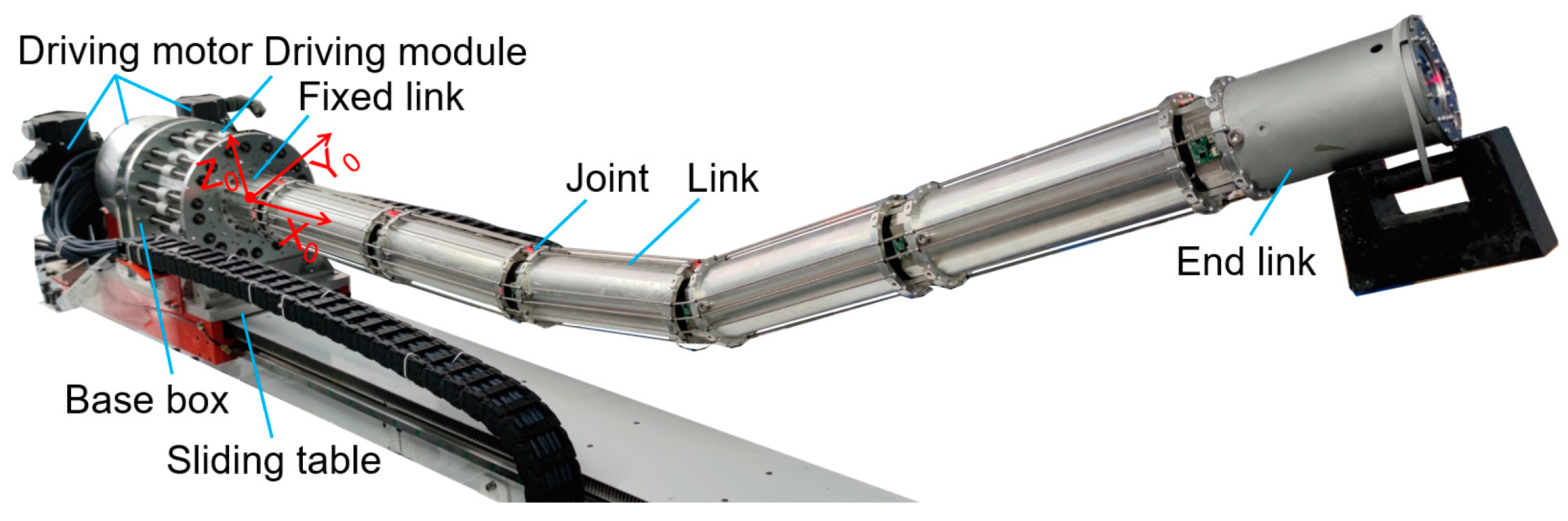
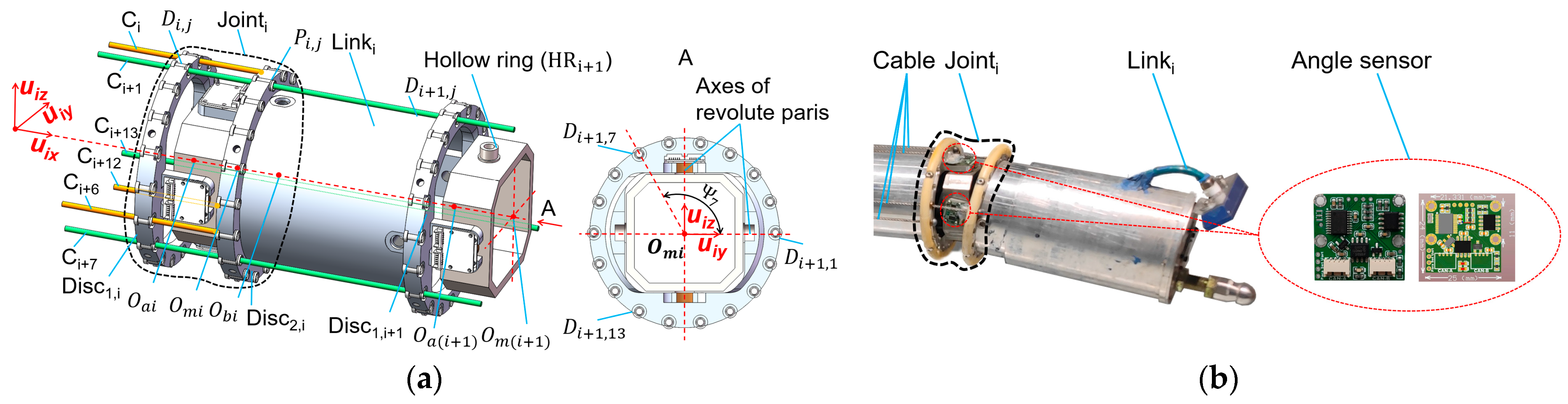
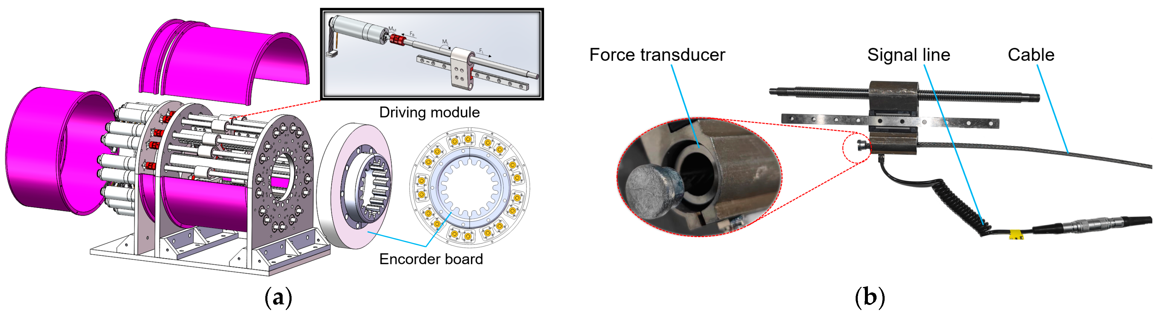
2. Mechanical Structure

The research object in this paper is a universal joint cable-driven snake-like robot with a mechanical structure shown in Figure 1. The structure can be divided into three parts: the sliding table, base box, and robot arm. The robot arm is driven by the cables, and the driving forces of the cables come from the driving modules of the base box.

The sliding table offers translation freedom for the base box and robot arm, expanding the workspace of the robot.

The detailed structure of the base box is shown in Figure 2. The driving module translates the motor power into the cable’s driving force, to drive the movement of the robot arm. The absolute encoders in the encoder board are used to monitor the positions of the driver modules. Figure 2b shows the setup of the force transducer, which is the key to achieving the dual-loop control.

The detailed structure of the robot arm is shown in Figure 3, which is composed by connecting universal joints and links in series. The CSR in the paper is with six universal joints and seven links. One link is a fixed link, which is denoted as $\mathrm{L}\mathrm{i}\mathrm{n}{\mathrm{k}}_0$ and connected to the base box. The remaining links are denoted as $\mathrm{L}\mathrm{i}\mathrm{n}{\mathrm{k}}_1\dots \mathrm{L}\mathrm{i}\mathrm{n}{\mathrm{k}}_6$ and the universal joints are denoted as $\mathrm{J}\mathrm{o}\mathrm{i}\mathrm{n}{\mathrm{t}}_1\dots \mathrm{J}\mathrm{o}\mathrm{i}\mathrm{n}{\mathrm{t}}_6$. Similarly, $\mathrm{J}\mathrm{o}\mathrm{i}\mathrm{n}{\mathrm{t}}_0$ means the fixed joint at the proximal end of $\mathrm{L}\mathrm{i}\mathrm{n}{\mathrm{k}}_0$. $\mathrm{J}\mathrm{o}\mathrm{i}\mathrm{n}{\mathrm{t}}_{\mathrm{i}}$’s key part $\mathrm{H}{\mathrm{R}}_{\mathrm{i}},$ i.e., the hollow ring, is used to connect two links. As shown in the figure, $\mathrm{J}\mathrm{o}\mathrm{i}\mathrm{n}{\mathrm{t}}_{\mathrm{i}}$ is driven by three yellow cables (${\mathrm{C}}_{\mathrm{i}},{\mathrm{C}}_{\mathrm{i}+6},{\mathrm{C}}_{\mathrm{i}+12}$) which are fixed on $\mathrm{L}\mathrm{i}\mathrm{n}{\mathrm{k}}_{\mathrm{i}}$. The three green cables (${\mathrm{C}}_{\mathrm{i}+1},{\mathrm{C}}_{\mathrm{i}+7},{\mathrm{C}}_{\mathrm{i}+7}$) which pass $\mathrm{L}\mathrm{i}\mathrm{n}{\mathrm{k}}_{\mathrm{i}}$ are fixed on $\mathrm{L}\mathrm{i}\mathrm{n}{\mathrm{k}}_{\mathrm{i}+1}$ and are to drive $\mathrm{J}\mathrm{o}\mathrm{i}\mathrm{n}{\mathrm{t}}_{\mathrm{i}+1}$ (though the figure shows only three cables passing through $\mathrm{L}\mathrm{i}\mathrm{n}{\mathrm{k}}_{\mathrm{i}}$, the cables driving $\mathrm{J}\mathrm{o}\mathrm{i}\mathrm{n}{\mathrm{t}}_{\mathrm{m}} \left(m>i\right)$ all pass through $\mathrm{L}\mathrm{i}\mathrm{n}{\mathrm{k}}_{\mathrm{i}}$). That means every universal joint is with two degrees of freedom and is driven by three cables. As shown in Figure 3b, each joint of the robot arm has been assembled with two angle sensors, which are also the key to achieving the dual-loop control.

3. Kinematics Modelling

As shown in Figure 1, the global coordinate system is constructed by: setting the proximal end of $\mathrm{L}\mathrm{i}\mathrm{n}{\mathrm{k}}_0$ as the origin; the vector from the proximal end to the distal end as the X₀-axis; the vector vertically upward as the Z₀-axis.

As shown in Figure 3, the center of $\mathrm{J}\mathrm{o}\mathrm{i}\mathrm{n}{\mathrm{t}}_{\mathrm{i}}$ is denoted as $O_{mi}$, which is also the proximal end of $\mathrm{L}\mathrm{i}\mathrm{n}{\mathrm{k}}_{\mathrm{i}}$. Then, $\mathrm{L}\mathrm{i}\mathrm{n}{\mathrm{k}}_{\mathrm{i}}$’s independent eigen vector can be defined as

$${\mathit{u}}_{\mathit{i}\mathit{x}}=\overrightarrow{O_{mi}{O}_{m\left(i+1\right)}}/\left|\overrightarrow{O_{mi}{O}_{m\left(i+1\right)}}\right|$$

(1)

According to the characteristics of the universal joint robot, the axes of the revolute pairs in the link can be set as the derived eigen vectors, which are denoted as ${\mathit{u}}_{\mathit{i}\mathit{y}}$, ${\mathit{u}}_{\mathit{i}\mathit{z}}$. That is to say, ${\mathit{u}}_{\mathit{i}\mathit{y}}$ coincides with the axis of the revolute pair between $\mathrm{L}\mathrm{i}\mathrm{n}{\mathrm{k}}_{\mathrm{i}}$ and $\mathrm{J}\mathrm{o}\mathrm{i}\mathrm{n}{\mathrm{t}}_{\mathrm{i}+1}$, ${\mathit{u}}_{\mathit{i}\mathit{z}}$ coincides with the axis of the revolute pair between $\mathrm{L}\mathrm{i}\mathrm{n}{\mathrm{k}}_{\mathrm{i}}$ and $\mathrm{J}\mathrm{o}\mathrm{i}\mathrm{n}{\mathrm{t}}_{\mathrm{i}}$. Then, the derived eigen vectors can be calculated by the following steps.

Let ${\mathit{u}}_{\mathit{d}\mathit{i}\mathit{r}\mathit{z}}={\mathit{u}}_{\mathit{i}\mathit{x}}\times {\mathit{u}}_{(\mathit{i}-1)\mathit{y}}$, then ${\mathit{u}}_{\mathit{d}\mathit{i}\mathit{r}\mathit{z}}$ is collinear with ${\mathit{u}}_{\mathit{i}\mathit{z}}$.

Let ${\mathit{u}}_{\mathit{d}\mathit{i}\mathit{r}\mathit{y}}={\mathit{u}}_{\mathit{d}\mathit{i}\mathit{r}\mathit{z}}\times {\mathit{u}}_{\mathit{i}\mathit{x}}$, then ${\mathit{u}}_{\mathit{d}\mathit{i}\mathit{r}\mathit{y}}$ is collinear with ${\mathit{u}}_{\mathit{i}\mathit{y}}$.

Thus, ${\mathit{u}}_{\mathit{i}\mathit{y}}$, ${\mathit{u}}_{\mathit{i}\mathit{z}}$ can be calculated by

$$\left\{\begin{array}{c}{\mathit{u}}_{\mathit{i}\mathit{z}}={\mathit{u}}_{\mathit{d}\mathit{i}\mathit{r}\mathit{z}}/\left|{\mathit{u}}_{\mathit{d}\mathit{i}\mathit{r}\mathit{z}}\right|\\ {\mathit{u}}_{\mathit{i}\mathit{y}}={\mathit{u}}_{\mathit{d}\mathit{i}\mathit{r}\mathit{y}}/\left|{\mathit{u}}_{\mathit{d}\mathit{i}\mathit{r}\mathit{y}}\right|\end{array}\right.$$

(2)

Therefore, the pose of $\mathrm{L}\mathrm{i}\mathrm{n}{\mathrm{k}}_{\mathrm{i}}$ can be completely described by the eigen vectors, ${{\mathit{u}}_{\mathit{i}\mathit{x}},\mathit{u}}_{\mathit{i}\mathit{y}}$, ${\mathit{u}}_{\mathit{i}\mathit{z}}$. Compared to the traditional kinematic models [17,23,24], which need to calculate the joint parameters with cumbersome methods and describe the pose information in many local coordinate systems, the link eigen vectors are more direct and intuitive.

As shown in Figure 3a, each joint has two discs, i.e., ${\mathrm{D}\mathrm{i}\mathrm{s}\mathrm{c}}_{1,\mathrm{i}}$, ${\mathrm{D}\mathrm{i}\mathrm{s}\mathrm{c}}_{2,\mathrm{i}}$. The centers of the discs are denoted as $O_{ai}$, $O_{bi},$ respectively. On one disc, 18 cable holes are evenly circumferentially distributed, which are for cables passing through. The cable hole on $\mathrm{D}\mathrm{i}\mathrm{s}{\mathrm{c}}_{1,\mathrm{i}+1}$ which is at ${\mathit{u}}_{\mathit{i}\mathit{y}}$ is denoted as $D_{i+1,1}$, and the remaining holes are counterclockwise denoted as $D_{i+1,2},D_{i+1,3}\dots D_{i+1,18}$. Similarly, the cable hole on $\mathrm{D}\mathrm{i}\mathrm{s}{\mathrm{c}}_{2,\mathrm{i}}$ which is at ${\mathit{u}}_{\mathit{i}\mathit{y}}$ is denoted as $P_{i,1}$, and the remaining holes are counterclockwise denoted as $P_{i,2},P_{i,3}\dots P_{i,18}$. The cables passing through the corresponding cable holes are denoted as ${\mathrm{C}}_1,{\mathrm{C}}_2\dots {\mathrm{C}}_{18}$. Let ${\Psi }_j$ refer to the included angle between $\overrightarrow{O_{ai}{D}_{i+1,j}}$ and ${\mathit{u}}_{\mathit{i}\mathit{y}}$ and also the included angle between $\overrightarrow{O_{bi}{P}_{i,j}}$ and ${\mathit{u}}_{\mathit{i}\mathit{y}}$, then

$${\Psi }_j=(j-1)\times \frac{2\pi }{3\times 6}$$

(3)

3.1. Mapping between Link Eigen Vectors and Cable Lengths

The cable ${\mathrm{C}}_{\mathrm{j}}$ can be divided into two parts, i.e., the link part and the joint part. When a cable is tensioned and the cable between two points is straight, the cable length between the two points is equal to the distance between the two points. Moreover, since the cable length in the link part remains constant, only the cable length in the joint part needs to be considered. Therefore, the theory cable length of ${\mathrm{C}}_{\mathrm{j}}$ in $\mathrm{J}\mathrm{o}\mathrm{i}\mathrm{n}{\mathrm{t}}_{\mathrm{i}}$ can be treated as the distance between $D_{i,j}$ and $P_{i,j}$,

$$s_{i,j}=\left|P_{i,j}-D_{i,j}\right|$$

(4)

$P_{i,j},D_{i,j}$ can be obtained by the following equations,

$$\left\{\begin{array}{c}{D}_{i,j}=P_{i-1,j}+O_{ai}-O_{b(i-1)}\\ P_{i,j}=r_d\cos \left({\Psi }_j\right){\mathit{u}}_{\mathit{i}\mathit{y}}+r_d\mathit{sin}\left({\Psi }_j\right){\mathit{u}}_{\mathit{i}\mathit{z}}+O_{bi}\end{array}\right.$$

(5)

$r_d:$ radius of the distribution circle of the hole on the disc.

$O_{ai},O_{bi}$ can be obtained by the following equations,

$$\left\{\begin{array}{c}{O}_{ai}=O_{mi}-d{\mathit{u}}_{\left(\mathit{i}-\mathbf{1}\right)\mathit{x}}\\ O_{bi}=O_{mi}+d{\mathit{u}}_{\mathit{i}\mathit{x}}\end{array}\right.(i=1,2\dots 6)$$

(6)

$d:$ distance from $O_{mi}$ to adjacent disc’s center, i.e., $d=\left|O_{mi}-O_{ai}\right|=\left|O_{mi}-O_{bi}\right|.$

The initial values of (5) are: $O_{b0}={\left[0 0 0\right]}^T,P_{0,j}={\left[0r_d\cos \left({\Psi }_j\right)r_d\sin \left({\Psi }_j\right)\right]}^T\left(j=1,2,\dots 18\right)$.

Let $C_{sj}$ be the pseudo total cable length of ${\mathrm{C}}_{\mathrm{j}}$, which is calculated by adding all corresponding $s_{i,j}$, then

$$C_{sj}={\sum }_{k=1}^{k=n_{j-1}+1}{s}_{k,j}$$

(7)

$n_j$: remainder of dividing $j$ by 6.

If the cable is tensioned, $C_{sj}$ can be taken as the real total cable’s length. Thus, the forward mapping is solved.

The inverse mapping can be divided into two situations, i.e., pseudo total cables’ lengths to link eigen vectors and real total cables’ lengths to link eigen vectors. Since the joint and link have sufficient stiffness, the first mapping is definite.

The first mapping, i.e., $C_{s1},\dots C_{s18}\to {\mathit{u}}_{\mathit{i}\mathit{x}},{\mathit{u}}_{\mathit{i}\mathit{y}},{\mathit{u}}_{\mathit{i}\mathit{z}}$, the values of $s_{m,n}\left(m=1,2\dots i-1\right),\left(n=i,i+6,i+12\right)$ can be solved from (4). And from (7), we can obtain,

$$\left\{\begin{array}{c}{s}_{i,i}=C_{si}-{\sum }_{k=1}^{k=n_{i-1}}{s}_{k,i}\\ s_{i,i+6}=C_{s(i+6)}-{\sum }_{k=1}^{k=n_{i+5}}{s}_{k,i+6}\\ s_{i,i+12}=C_{s(i+12)}-{\sum }_{k=1}^{k=n_{i+11}}{s}_{k,i+12}\end{array}\right.$$

(8)

Since ${\mathit{u}}_{\mathit{i}\mathit{x}}$ is a unit vector, ${\mathit{u}}_{\mathit{i}\mathit{x}}$ can be set as ${\left[\mathrm{c}\mathrm{o}\mathrm{s}{\gamma }_i,\mathrm{s}\mathrm{i}\mathrm{n}{\gamma }_i\mathrm{c}\mathrm{o}\mathrm{s}{\phi }_i,\mathrm{s}\mathrm{i}\mathrm{n}{\gamma }_i\mathrm{s}\mathrm{i}\mathrm{n}{\phi }_i\right]}^T({\phi }_i\in [0,2\pi ],{\gamma }_i\in [0,\pi \left)\right)$. Then, substituting the expression of ${\mathit{u}}_{\mathit{i}\mathit{x}}$ into (2), we can obtain,

$${\mathit{u}}_{\mathit{i}\mathit{z}}={\mathit{u}}_{\mathit{d}\mathit{i}\mathit{r}\mathit{z}}/\left|{\mathit{u}}_{\mathit{d}\mathit{i}\mathit{r}\mathit{z}}\right|={(\mathit{u}}_{\mathit{i}\mathit{x}}\times {\mathit{u}}_{\left(\mathit{i}-\mathbf{1}\right)\mathit{y}})/|{\mathit{u}}_{\mathit{i}\mathit{x}}\times {\mathit{u}}_{\left(\mathit{i}-\mathbf{1}\right)\mathit{y}}|=(f_{iz}\left({\phi }_i,{\gamma }_i\right),g_{iz}\left({\phi }_i,{\gamma }_i\right),h_{iz}{(\phi }_i,{\gamma }_i\left)\right)$$

(9)

$f_{iz}\left({\phi }_i,{\gamma }_i\right),g_{iz}\left({\phi }_i,{\gamma }_i\right),h_{iz}\left({\phi }_i,{\gamma }_i\right)$: X, Y, Z coordinates of ${\mathit{u}}_{\mathit{i}\mathit{z}}$, which are expressed by the variables ${\phi }_i$ and ${\gamma }_i$.

Similarly,

$${\mathit{u}}_{\mathit{i}\mathit{y}}=(f_{iy}\left({\phi }_i,{\gamma }_i\right),g_{iy}\left({\phi }_i,{\gamma }_i\right),h_{iy}\left({\phi }_i,{\gamma }_i\right))$$

(10)

$f_{iy}\left({\phi }_i,{\gamma }_i\right),g_{iy}\left({\phi }_i,{\gamma }_i\right),h_{iy}\left({\phi }_i,{\gamma }_i\right)$: X, Y, Z coordinates of ${\mathit{u}}_{\mathit{i}\mathit{y}}$, which are also expressed by the variables ${\phi }_i$ and ${\gamma }_i$.

Thus, the expressions of ${\mathit{u}}_{\mathit{i}\mathit{y}},{\mathit{u}}_{\mathit{i}\mathit{z}}$ also have two variables. Substitute the above ${\mathit{u}}_{\mathit{i}\mathit{x}},{\mathit{u}}_{\mathit{i}\mathit{y}},{\mathit{u}}_{\mathit{i}\mathit{z}}$ into (4)–(6), we can obtain,

$$\left\{\begin{array}{c}{s}_{i,i}=F_{s_i}({\phi }_i,{\gamma }_i)\\ s_{i,i+6}=F_{s_{i+6}}({\phi }_i,{\gamma }_i)\\ s_{i,i+12}=F_{s_{i+12}}({\phi }_i,{\gamma }_i)\end{array}\right.$$

(11)

Then, the expressions of $s_{i,i}, s_{i,i+6}, s_{i,i+12}$ also have two variables, ${\phi }_i,{\gamma }_i$. Since the values of $s_{i,i}, s_{i,i+6}, s_{i,i+12}$ are already calculated through (8), the following equations with two unknown variables can be obtained,

$$\left\{\begin{array}{c}{F}_{s_i}\left({\phi }_i,{\gamma }_i\right)=C_{si}-{\sum }_{k=1}^{k=n_{i-1}}{s}_{k,i}\\ F_{s_{i+6}}\left({\phi }_i,{\gamma }_i\right)=C_{s(i+6)}-{\sum }_{k=1}^{k=n_{i+5}}{s}_{k,i+6}\\ F_{s_{i+12}}\left({\phi }_i,{\gamma }_i\right)=C_{s(i+12)}-{\sum }_{k=1}^{k=n_{i+11}}{s}_{k,i+12}\end{array}\right.$$

(12)

As the stiffness of the joints is enough, the above equations have a consistent solution within the accuracy range. Therefore, it is reasonable to use any two of the above equations to calculate the values of ${\phi }_i$ and ${\gamma }_i$, to obtain the values of ${\mathit{u}}_{\mathit{i}\mathit{x}},{\mathit{u}}_{\mathit{i}\mathit{y}},{\mathit{u}}_{\mathit{i}\mathit{z}}$. Since the equations are complex, the Newton–Raphson method could be used for the numerical solution.

When ${\mathit{u}}_{\mathit{i}\mathit{x}}={\mathit{u}}_{(\mathit{i}-\mathbf{1})\mathit{x}}$, the values of ${\phi }_i,{\gamma }_i$ could be set as initial values. Then, ${\phi }_i,{\gamma }_i$ can be solved by the iterative method. Additionally, the solved ${\phi }_i,{\gamma }_i$ can be substituted into the last equation of (12) for verification. And if the left and right sides of (12) are equal within the acceptable error range, ${\mathit{u}}_{\mathit{i}\mathit{x}},{\mathit{u}}_{\mathit{i}\mathit{y}},{\mathit{u}}_{\mathit{i}\mathit{z}}$ are solved successfully. On the contrary, there is no solution. Then, $O_{m(i+1)}$ can be solved as follows,

$$O_{m(i+1)}=l_i{\mathit{u}}_{\mathit{i}\mathit{x}}+O_{mi}$$

(13)

$l_i:$ length of $Lin{k}_i$, $l_i=\left|\overrightarrow{O_{mi}{O}_{m\left(i+1\right)}}\right|$.

In the second mapping situation of calculating ${\mathit{u}}_{\mathit{i}\mathit{x}},{\mathit{u}}_{\mathit{i}\mathit{y}},{\mathit{u}}_{\mathit{i}\mathit{z}}$, there are three more subcases:

(1)

Every cable is tensioned. Then, the cables’ lengths are approximately equal to the distances between corresponding holes, so the inverse mapping method is the same as the first mapping method.

(2)

Two of the cables that drive the joint are tensioned, but the other is slack. Then, the two cables’ lengths are approximately equal to the distances between the corresponding holes. Thus, compared to the first mapping situation’s method, just the verification equation is canceled.

(3)

More than one of the cables is slack. In this case, the inverse mapping cannot be performed.

It is worthy noting that the effects of $\mathrm{J}\mathrm{o}\mathrm{i}\mathrm{n}{\mathrm{t}}_1,\dots \mathrm{J}\mathrm{o}\mathrm{i}\mathrm{n}{\mathrm{t}}_{\mathrm{i}-1}$ to the lengths of the cables must be considered before the inverse mapping in $\mathrm{J}\mathrm{o}\mathrm{i}\mathrm{n}{\mathrm{t}}_{\mathrm{i}}$.

3.2. Mapping between Link Eigen Vectors and Joint Angles

In the new kinematic model, the joint parameters are not necessary. However, as it is convenient to obtain the pose of CSR with the utilization of joint angle sensors, the mapping relation between the link eigen vectors and the joint angles is derived here. Set the joint angle of the revolute pair between $\mathrm{L}\mathrm{i}\mathrm{n}{\mathrm{k}}_{\mathrm{i}-1}$ and $\mathrm{J}\mathrm{o}\mathrm{i}\mathrm{n}{\mathrm{t}}_{\mathrm{i}}$ as ${\alpha }_i$ and the joint angle of the revolute pair between $\mathrm{J}\mathrm{o}\mathrm{i}\mathrm{n}{\mathrm{t}}_{\mathrm{i}}$ and $\mathrm{L}\mathrm{i}\mathrm{n}{\mathrm{k}}_{\mathrm{i}}$ as ${\beta }_i$. When ${\mathit{u}}_{\mathit{i}\mathit{x}}={\mathit{u}}_{\left(\mathit{i}-\mathbf{1}\right)\mathit{x}}$, set ${\alpha }_i={\beta }_i=0$. Then

(1)

Forward mapping, $({\mathit{u}}_{\mathit{i}\mathit{x}},{\mathit{u}}_{\mathit{i}\mathit{y}},{\mathit{u}}_{\mathit{i}\mathit{z}})\to ({\alpha }_i,{\beta }_i)$.

Let

$$\left\{\begin{array}{c}Pro{j}_x={\mathit{u}}_{\mathit{i}\mathit{x}}·{\mathit{u}}_{\left(\mathit{i}-\mathbf{1}\right)\mathit{x}}\\ Pro{j}_y={\mathit{u}}_{\mathit{i}\mathit{x}}·{\mathit{u}}_{\left(\mathit{i}-\mathbf{1}\right)\mathit{y}}\\ Pro{j}_z={\mathit{u}}_{\mathit{i}\mathit{x}}·{\mathit{u}}_{\left(\mathit{i}-\mathbf{1}\right)\mathit{z}}\end{array}\right.$$

(14)

Thus, we can obtain,

$$\left\{\begin{array}{c}{\alpha }_i=-\arctan \left(Pro{j}_z/Pr{o}_x\right){\alpha }_i\in (-0.5\pi ,0.5\pi )\\ {\beta }_i=\arcsin \left(Pro{j}_y\right){\beta }_i\in (-0.5\pi ,0.5\pi )\end{array}\right.$$

(15)

(2)

Inverse mapping, $\left({\alpha }_i,{\beta }_i\right)\to ({\mathit{u}}_{\mathit{i}\mathit{x}},{\mathit{u}}_{\mathit{i}\mathit{y}},{\mathit{u}}_{\mathit{i}\mathit{z}})$.

Let

$$\left\{\begin{array}{c}{\mathit{v}}_{\mathit{i}\mathit{y}}={\mathit{u}}_{\left(\mathit{i}-\mathbf{1}\right)\mathit{y}}\\ {\mathit{v}}_{\mathit{i}\mathit{z}}=\cos \left({\alpha }_i\right){\mathit{u}}_{\left(\mathit{i}-\mathbf{1}\right)\mathit{z}}+\sin \left({\alpha }_i\right){\mathit{u}}_{\left(\mathit{i}-\mathbf{1}\right)\mathit{x}}\\ {\mathit{v}}_{\mathit{i}\mathit{x}}={\mathit{v}}_{\mathit{i}\mathit{y}}\times {\mathit{v}}_{\mathit{i}\mathit{z}}\end{array}\right.$$

(16)

Thus, we can obtain,

$$\left\{\begin{array}{c}{\mathit{u}}_{\mathit{i}\mathit{z}}={\mathit{v}}_{\mathit{i}\mathit{z}}\\ {\mathit{u}}_{\mathit{i}\mathit{x}}=\cos \left({\beta }_i\right){\mathit{v}}_{\mathit{i}\mathit{x}}+\mathit{sin}\left({\beta }_i\right){\mathit{v}}_{\mathit{i}\mathit{y}}\\ {\mathit{u}}_{\mathit{i}\mathit{y}}={\mathit{u}}_{\mathit{i}\mathit{z}}\times {\mathit{u}}_{\mathit{i}\mathit{x}}\end{array}\right.$$

(17)

The key part of $\mathrm{J}\mathrm{o}\mathrm{i}\mathrm{n}{\mathrm{t}}_{\mathrm{i}}$, $\mathrm{H}{\mathrm{R}}_{\mathrm{i}}$ also has its eigen vectors, which are exactly ${\mathit{v}}_{\mathit{i}\mathit{x}},{\mathit{v}}_{\mathit{i}\mathit{y}},{\mathit{v}}_{\mathit{i}\mathit{z}}$. All eigen vectors of the hollow ring can be calculated by link eigen vectors.

4. Inverse Dynamics

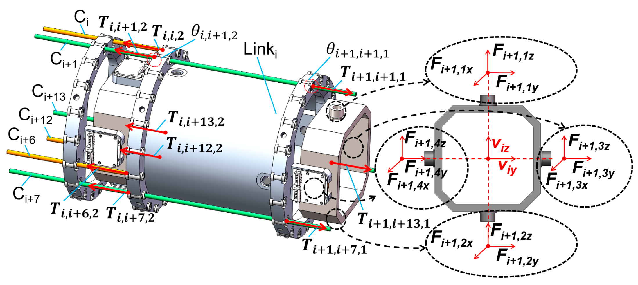
4.1. Mechanical Analysis

As shown in Figure 4, ${\mathrm{C}}_{\mathrm{i}},{\mathrm{C}}_{\mathrm{i}+6},{\mathrm{C}}_{\mathrm{i}+12}$ are fixed on $\mathrm{L}\mathrm{i}\mathrm{n}{\mathrm{k}}_{\mathrm{i}}$. They provide the driving forces for $\mathrm{L}\mathrm{i}\mathrm{n}{\mathrm{k}}_{\mathrm{i}}$’s movement. At the same time, the cables passing through $\mathrm{L}\mathrm{i}\mathrm{n}{\mathrm{k}}_{\mathrm{i}}$ also have forces acting on $\mathrm{L}\mathrm{i}\mathrm{n}{\mathrm{k}}_{\mathrm{i}}$ (Figure 4 only shows three cables passing through $\mathrm{L}\mathrm{i}\mathrm{n}{\mathrm{k}}_{\mathrm{i}}$, i.e., ${\mathrm{C}}_{\mathrm{i}+1},{\mathrm{C}}_{\mathrm{i}+7},{\mathrm{C}}_{\mathrm{i}+13}$). These cables are fixed on $\mathrm{L}\mathrm{i}\mathrm{n}{\mathrm{k}}_{\mathrm{m}}(i<m\le 6)$.

Suppose the turning angle of ${\mathrm{C}}_{\mathrm{i}+1}$ at $P_{i,i+1}$ is ${\theta }_{i,i+1,2}$ and the turning angle of ${\mathrm{C}}_{\mathrm{i}+1}$ at $D_{i+1,i+1}$ is ${\theta }_{i+1,i+1,1}$, then

$$|{\mathit{T}}_{\mathit{i}+\mathbf{1},\mathit{i}+\mathbf{1},\mathbf{1}}/{\mathit{T}}_{\mathit{i},\mathit{i}+\mathbf{1},\mathbf{2}}|=e^{\mu {\theta }_{i,i+1,1}}{·e}^{\mu {\theta }_{i,j,2}}$$

(18)

$\mu$: Coulomb friction coefficient.

${\mathit{T}}_{\mathit{i}+\mathbf{1},\mathit{i}+\mathbf{1},\mathbf{1}}$: cable force of ${\mathrm{C}}_{\mathrm{i}+1}$ in $\mathrm{J}\mathrm{o}\mathrm{i}\mathrm{n}{\mathrm{t}}_{\mathrm{i}+1}$, whose direction is shown in Figure 4.

${\mathit{T}}_{\mathit{i},\mathit{i}+\mathbf{1},\mathbf{2}}$: cable force of ${\mathrm{C}}_{\mathrm{i}+1}$ in $\mathrm{J}\mathrm{o}\mathrm{i}\mathrm{n}{\mathrm{t}}_{\mathrm{i}}$, ${\mathit{T}}_{\mathit{i},\mathit{i}+\mathbf{1},\mathbf{2}}=-{\mathit{T}}_{\mathit{i},\mathit{i}+\mathbf{1},\mathbf{1}}$.

Let

$$\left\{\begin{array}{c}{\mathit{v}}_{\mathit{i},j,\mathbf{1}}={(D}_{i,j}-P_{i,j})/|D_{i,j}-P_{i,j}|\\ {\mathit{v}}_{\mathit{i},j,\mathbf{2}}=(P_{i,j}-D_{i+1,j})/|P_{i,j}-D_{i+1,j}|\end{array}\right.$$

(19)

Then

$$\left\{\begin{array}{c}{\theta }_{i,j,1}={\cos }^{-1}({\mathit{v}}_{\mathit{i},j,\mathbf{1}}·{\mathit{v}}_{\mathit{i},j,\mathbf{2}})\\ {\theta }_{i,j,2}={\cos }^{-1}({\mathit{v}}_{\mathit{i},j,\mathbf{2}}·{\mathit{v}}_{\mathit{i}+\mathbf{1},j,\mathbf{1}})\end{array}\right.$$

(20)

As a result, if the cable force of a cable in a joint is known, all cable forces of the cable in the other joints can be calculated. Since the mechanics analysis of the robot is an inward recursion, $\mathrm{L}\mathrm{i}\mathrm{n}{\mathrm{k}}_{\mathrm{m}}$’s $(m>i)$ force analysis is before $\mathrm{L}\mathrm{i}\mathrm{n}{\mathrm{k}}_{\mathrm{i}}$. Therefore, the cable forces of the cables passing through $\mathrm{L}\mathrm{i}\mathrm{n}{\mathrm{k}}_{\mathrm{i}}$ are known, on the contrary, the cable forces of the cables fixed on $\mathrm{L}\mathrm{i}\mathrm{n}{\mathrm{k}}_{\mathrm{i}}$ are the driving forces to be solved.

For $\mathrm{H}{\mathrm{R}}_{\mathrm{i}}$, $O_{mi}$ is the center of mass. The acting forces on $\mathrm{H}{\mathrm{R}}_{\mathrm{i}}$ are:

(1)

The acting forces from distal $\mathrm{L}\mathrm{i}\mathrm{n}{\mathrm{k}}_{\mathrm{i}}$, ${\mathit{F}}_{\mathit{i},\mathbf{1}},{\mathit{F}}_{\mathit{i},\mathbf{2}}$. They can be decomposed into six forces with known action lines and directions, ${\mathit{F}}_{\mathit{i},\mathbf{1}\mathit{x}},{\mathit{F}}_{\mathit{i},\mathbf{1}\mathit{y}},{\mathit{F}}_{\mathit{i},\mathbf{1}\mathit{z}},{\mathit{F}}_{\mathit{i},\mathbf{2}\mathit{x}},{\mathit{F}}_{\mathit{i},\mathbf{2}\mathit{y}},{\mathit{F}}_{\mathit{i},\mathbf{2}\mathit{z}}$. The moment of them about $O_{mi}$ is denoted as ${\mathit{M}}_{\mathbf{1},\mathbf{2}}^{}$.

(2)

The acting forces from $\mathrm{L}\mathrm{i}\mathrm{n}{\mathrm{k}}_{\mathrm{i}-1}$, ${\mathit{F}}_{\mathit{i},\mathbf{3}},{\mathit{F}}_{\mathit{i},\mathbf{4}}$. Similarly, they can also be decomposed into six forces with known action lines and directions, ${\mathit{F}}_{\mathit{i},\mathbf{3}\mathit{x}},{\mathit{F}}_{\mathit{i},\mathbf{3}\mathit{y}},{\mathit{F}}_{\mathit{i},\mathbf{3}\mathit{z}},{\mathit{F}}_{\mathit{i},\mathbf{4}\mathit{x}},{\mathit{F}}_{\mathit{i},\mathbf{4}\mathit{y}},{\mathit{F}}_{\mathit{i},\mathbf{4}\mathit{z}}$. The moment of them about $O_{mi}$ is denoted as ${\mathit{M}}_{\mathbf{3},\mathbf{4}}^{}$.

(3)

Gravity force, ${\mathit{G}}_{\mathit{H}\mathit{i}}$.

(4)

Inertia force and moment, ${\mathit{F}}_{\mathit{I}\mathit{H},\mathit{i}},{\mathit{M}}_{\mathit{I}\mathit{H},\mathit{i}}$.

Since ${\mathit{F}}_{\mathit{i},\mathbf{1}\mathit{z}},{\mathit{F}}_{\mathit{i},\mathbf{2}\mathit{z}}$ act on the same line, they can be merged as

$${\mathit{F}}_{\mathit{i},\mathit{z}\mathit{c}}={\mathit{F}}_{\mathit{i},\mathbf{1}\mathit{z}}+{\mathit{F}}_{\mathit{i},\mathbf{2}\mathit{z}}$$

(21)

Thus, ${\mathit{F}}_{\mathit{i},\mathbf{1}},{\mathit{F}}_{\mathit{i},\mathbf{2}}$ can be simplified as five forces with known action lines and directions.

Similarly, ${\mathit{F}}_{\mathit{i},\mathbf{3}\mathit{y}},{\mathit{F}}_{\mathit{i},\mathbf{4}\mathit{y}}$ can be merged as,

$${\mathit{F}}_{\mathit{i},\mathit{y}\mathit{c}}={\mathit{F}}_{\mathit{i},\mathbf{3}\mathit{y}}+{\mathit{F}}_{\mathit{i},\mathbf{4}\mathit{y}}$$

(22)

Thus, ${\mathit{F}}_{\mathit{i},\mathbf{3}\mathit{y}},{\mathit{F}}_{\mathit{i},\mathbf{4}\mathit{y}}$ can also be simplified as five forces with known action lines and directions.

According to the current values and historical values of $O_{mi}$ and $\mathrm{H}{\mathrm{R}}_{\mathrm{i}}$’s eigen vectors ${\mathit{v}}_{\mathit{i}\mathit{x}},{\mathit{v}}_{\mathit{i}\mathit{y}},{\mathit{v}}_{\mathit{i}\mathit{z}}$, the velocity ${\mathit{v}}_{\mathit{c}\mathit{H},\mathit{i}}$, acceleration ${\mathit{a}}_{\mathit{c}\mathit{c}\mathit{H},\mathit{i}}$, angular velocity ${\mathit{\omega }}_{\mathit{H}\mathit{i}}$ and angular acceleration ${\mathit{\alpha }}_{\mathit{H}\mathit{i}}$ of $\mathrm{H}{\mathrm{R}}_{\mathrm{i}}$ at the centroid can be calculated. Thus, the values of ${\mathit{F}}_{\mathit{I}\mathit{H},\mathit{i}},{\mathit{M}}_{\mathit{I}\mathit{H},\mathit{i}}$ are

$${\mathit{F}}_{\mathit{I}\mathit{H},\mathit{i}}=-m_{Hi}·{\mathit{a}}_{\mathit{c}\mathit{c}\mathit{H},\mathit{i}}$$

(23)

$${\mathit{M}}_{\mathit{I}\mathit{H},\mathit{i}}=-{\mathit{I}}_{\mathit{c}\mathit{H},\mathit{i}}{\mathit{\alpha }}_{\mathit{H}\mathit{i}}-{\mathit{\omega }}_{\mathit{H}\mathit{i}}\times {(\mathit{I}}_{\mathit{c}\mathit{H},\mathit{i}}{\mathit{\omega }}_{\mathit{H}\mathit{i}})$$

(24)

$m_{Hi}$: mass of $\mathrm{H}{\mathrm{R}}_{\mathrm{i}}$.

${\mathit{I}}_{\mathit{c}\mathit{H},\mathit{i}}$: inertia tensor of $\mathrm{H}{\mathrm{R}}_{\mathrm{i}}$ relative to the center of mass in the global coordinate system.

The acting forces on $\mathrm{L}\mathrm{i}\mathrm{n}{\mathrm{k}}_{\mathrm{i}}$ are:

(1)

The known cable forces ${\mathit{S}}_{\mathit{T}\mathbf{1},\mathit{i}}$ from the cables which are fixed on $\mathrm{L}\mathrm{i}\mathrm{n}{\mathrm{k}}_{\mathrm{m}}(m>i)$. The moment of them about $O_{mi}$ is denoted as ${\mathit{S}}_{\mathit{M}\mathit{T}\mathbf{1},\mathit{i}}$.

(2)

The unknown cable forces ${\mathit{S}}_{\mathit{T}\mathbf{2},\mathit{i}}$ from the cables which are fixed on $\mathrm{L}\mathrm{i}\mathrm{n}{\mathrm{k}}_{\mathrm{i}}$. The moment of them about $O_{mi}$ is denoted as ${\mathit{S}}_{\mathit{M}\mathit{T}\mathbf{2},\mathit{i}}$.

(3)

The acting forces from distal $\mathrm{H}{\mathrm{R}}_{\mathrm{i}+1}$, ${-\mathit{F}}_{\mathit{i}+\mathbf{1},\mathbf{3}},-{\mathit{F}}_{\mathit{i}+\mathbf{1},\mathbf{4}}$ (if $\mathrm{L}\mathrm{i}\mathrm{n}{\mathrm{k}}_{\mathrm{i}}$ is the end link, the forces can be taken as environment forces). The moment of the forces about $O_{mi}$ is set as $-{\mathit{M}}_{\mathbf{3},\mathbf{4}}^{\mathbf{\prime }}$.

(4)

The acting forces from proximal $\mathrm{H}{\mathrm{R}}_{\mathrm{i}}$, ${-\mathit{F}}_{\mathit{i},\mathbf{1}},{-\mathit{F}}_{\mathit{i},\mathbf{2}}$. The moment of the forces about $O_{mi}$ is denoted as $-{\mathit{M}}_{\mathbf{1},\mathbf{2}}^{}$.

(5)

Gravity force, ${\mathit{G}}_{\mathit{i}}$. The moment of the force about $O_{mi}$ is denoted as ${\mathit{M}}_{{\mathit{G}}_{\mathit{i}}}$.

(6)

Inertia force and moment, ${\mathit{F}}_{\mathit{I},\mathit{i}}$, ${\mathit{M}}_{\mathit{I},\mathit{i}}$. The moment of ${\mathit{F}}_{\mathit{I},\mathit{i}}$ about $O_{mi}$ is denoted as ${{\mathit{M}}_{\mathit{F}}}_{\mathit{I},\mathit{i}}$.

The position of $\mathrm{L}\mathrm{i}\mathrm{n}{\mathrm{k}}_{\mathrm{i}}$’s centroid relative to $O_{mi}$ is known. Then, according to the current values and historical values of $O_{mi}$ and $\mathrm{L}\mathrm{i}\mathrm{n}{\mathrm{k}}_{\mathrm{i}}$’s eigen vectors ${\mathit{u}}_{\mathit{i}\mathit{x}},{\mathit{u}}_{\mathit{i}\mathit{y}},{\mathit{u}}_{\mathit{i}\mathit{z}}$, the velocity ${\mathit{v}}_{\mathit{c},\mathit{i}}$, acceleration ${\mathit{a}}_{\mathit{c}\mathit{c},\mathit{i}}$, angular velocity ${\mathit{\omega }}_{\mathit{i}}$ and angular acceleration ${\mathit{\alpha }}_{\mathit{i}}$ of $\mathrm{L}\mathrm{i}\mathrm{n}{\mathrm{k}}_{\mathrm{i}}$ at the centroid can be calculated [31]. Thus, the values of ${\mathit{F}}_{\mathit{I},\mathit{i}},{\mathit{M}}_{\mathit{I},\mathit{i}}$ are

$${\mathit{F}}_{\mathit{I},\mathit{i}}=-m_i·{\mathit{a}}_{\mathit{c}\mathit{c},\mathit{i}}$$

(25)

$${\mathit{M}}_{\mathit{I},\mathit{i}}=-{\mathit{I}}_{\mathit{c},\mathit{i}}{\mathit{\alpha }}_{\mathit{i}}-{\mathit{\omega }}_{\mathit{i}}\times {(\mathit{I}}_{\mathit{c},\mathit{i}}{\mathit{\omega }}_{\mathit{i}})$$

(26)

$m_i:$ mass of $\mathrm{L}\mathrm{i}\mathrm{n}{\mathrm{k}}_{\mathrm{i}}$.

${\mathit{I}}_{\mathit{c},\mathit{i}}$: inertia tensor of $\mathrm{L}\mathrm{i}\mathrm{n}{\mathrm{k}}_{\mathrm{i}}$ relative to the center of mass in the global coordinate system.

4.2. Newton–Euler Method

According to the mechanical analysis, the Newton–Euler equations of $\mathrm{H}{\mathrm{R}}_{\mathrm{i}}$ are

$$\left\{\begin{array}{c}{\mathit{F}}_{\mathit{i},\mathbf{1}}+{\mathit{F}}_{\mathit{i},\mathbf{2}}{+\mathit{F}}_{\mathit{i},\mathbf{3}}+{\mathit{F}}_{\mathit{i},\mathbf{4}}+{\mathit{G}}_{\mathit{H}\mathit{i}}+{\mathit{F}}_{\mathit{I}\mathit{H},\mathit{i}}=\mathbf{0}\\ {\mathit{M}}_{\mathbf{1},\mathbf{2}}^{}+{\mathit{M}}_{\mathbf{3},\mathbf{4}}^{}+{\mathit{M}}_{\mathit{I}\mathit{H},\mathit{i}}=\mathbf{0}\end{array}\right.$$

(27)

The Newton–Euler equations of $\mathrm{L}\mathrm{i}\mathrm{n}{\mathrm{k}}_{\mathrm{i}}$ are

$$\left\{\begin{array}{c}{{{\mathit{S}}_{\mathit{T}\mathbf{1},\mathit{i}}+{\mathit{S}}_{\mathit{T}\mathbf{2},\mathit{i}}-\mathit{F}}_{\mathit{i},\mathbf{1}}{-\mathit{F}}_{\mathit{i},\mathbf{2}}-\mathit{F}}_{\mathit{i}+\mathbf{1},\mathbf{3}}-{\mathit{F}}_{\mathit{i}+\mathbf{1},\mathbf{4}}+{\mathit{G}}_{\mathit{i}}+{\mathit{F}}_{\mathit{I},\mathit{i}}=\mathbf{0}\\ {\mathit{S}}_{\mathit{M}\mathit{T}\mathbf{1},\mathit{i}}+{\mathit{S}}_{\mathit{M}\mathit{T}\mathbf{2},\mathit{i}}-{\mathit{M}}_{\mathbf{1},\mathbf{2}}^{}-{\mathit{M}}_{\mathbf{3},\mathbf{4}}^{\prime }+{\mathit{M}}_{{\mathit{G}}_{\mathit{i}}}+{\mathit{M}}_{\mathit{I},\mathit{i}}+{{\mathit{M}}_{\mathit{F}}}_{\mathit{I},\mathit{i}}=\mathbf{0}\end{array}\right.$$

(28)

In the above equations, the variables to be solved are ${\mathit{F}}_{\mathit{i},\mathbf{1}},{\mathit{F}}_{\mathit{i},\mathbf{2}}{,\mathit{F}}_{\mathit{i},\mathbf{3}},{\mathit{F}}_{\mathit{i},\mathbf{4}},{\mathit{S}}_{\mathit{T}\mathbf{2},\mathit{i}}$. ${\mathit{F}}_{\mathit{i},\mathbf{1}},{\mathit{F}}_{\mathit{i},\mathbf{2}}{,\mathit{F}}_{\mathit{i},\mathbf{3}},{\mathit{F}}_{\mathit{i},\mathbf{4}}$ can be decomposed into 10 forces with known action lines and directions. ${\mathit{S}}_{\mathit{T}\mathbf{2},\mathit{i}}$ can be decomposed into 3 forces with known action lines and directions. Therefore, (27) and (28) are with 12 independent equations and 13 unknown variables. Let the smallest force of ${\mathit{S}}_{\mathit{T}\mathbf{2},\mathit{i}}$ be equal to the pre-tensioning force ${\mathit{T}}_{\mathit{p}\mathit{r}\mathit{e}}$, then the needed driving forces of the cables can be solved. Thus, the inverse dynamics is resolved.

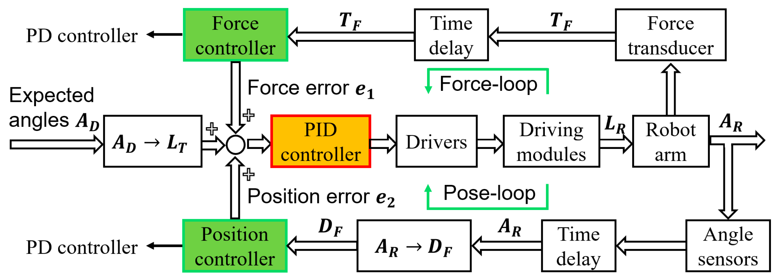
5. Dual-Loop Control Strategy

5.1. Errors Analysis

Cable zero length (CZL) refers to a cable length when the arm of CSR stays straight and horizontal. CZL is calculated without the model error. For convenience, the cable lengths discussed in this section are all relative to the cable zero lengths.

Cable real lengths, ${\mathit{L}}_{\mathit{R}}$, refer to the differences in the real cable lengths relative to the CZLs after the joints rotate at certain angles.

Cable theory lengths, ${\mathit{L}}_{\mathit{T}}$, refer to the differences in the theory cable lengths relative to the CZLs after the joints rotate at certain angles. Note that theory cable lengths are calculated by adding the distances between two groups of corresponding cable holes. It is called theory lengths due to the errors between ${\mathit{L}}_{\mathit{T}}$ and ${\mathit{L}}_{\mathit{R}}$. There are four main errors:

The first errors ${\mathit{E}}_{\mathit{f}\mathit{i}\mathit{r}}$: When a cable passes a link, it passes the cable holes. As the inner diameter of the cable hole is larger than the diameter of the cable, the cable has a radial movement relative to the cable hole. However, ${\mathit{L}}_{\mathit{T}}$ is calculated assuming that the cable is always at the center of the cable hole. Take cable ${\mathrm{C}}_1$ in $\mathrm{J}\mathrm{o}\mathrm{i}\mathrm{n}{\mathrm{t}}_1$’s part as an example (the other cables and joints have similar error relations). As shown in Figure 5, the left figure is the relation among ${\mathit{L}}_{\mathit{T}}$, $\gamma ,$ and $\varnothing$, and the right figure is the relation among ${\mathit{E}}_{\mathit{f}\mathit{i}\mathit{r}}$, $\gamma ,$ and $\varnothing$. The $\gamma$ refers to the included angle between ${\mathit{X}}_{\mathbf{0}}$ and ${\mathit{u}}_{\mathbf{1}\mathit{x}}$, i.e., the included angle between ${\mathit{u}}_{\mathbf{0}\mathit{x}}$ and ${\mathit{u}}_{\mathbf{1}\mathit{x}}$. $\varnothing$ refers to the included angle between the projection of ${\mathit{u}}_{\mathbf{1}\mathit{x}}$ in the plane $X_0{Y}_0$ and ${\mathit{Y}}_{\mathbf{0}}$.

The second errors ${\mathit{E}}_{\mathit{s}\mathit{e}\mathit{c}}$: The distance of $\mathrm{J}\mathrm{o}\mathrm{i}\mathrm{n}{\mathrm{t}}_{\mathrm{i}}$’s center to the adjacent discs’ center, which is denoted as $d$ in the above section, will slightly vary due to the change in the tension of the cables. Therefore, only a theoretical approximation can be taken as this distance. Again, take the cable ${\mathrm{C}}_1$ in $\mathrm{J}\mathrm{o}\mathrm{i}\mathrm{n}{\mathrm{t}}_1$’s part as an example. As shown in Figure 6, the left figure is the relation among ${\mathit{L}}_{\mathit{R}}$, $\gamma$ and $\mathrm{\varnothing }$. The right figure is the relation among ${\mathit{E}}_{\mathit{s}\mathit{e}\mathit{c}}$, $\gamma$ and $\mathrm{\varnothing }$.

The third errors ${\mathit{E}}_{\mathit{t}\mathit{h}\mathit{i}}$: When the cable is under tension, it will be stretched and deformed, and its length will change. However, the errors are minor and can be eliminated according to the feedback values of the force transducers.

The fourth errors ${\mathit{E}}_{\mathit{f}\mathit{o}\mathit{u}}$: These errors are caused by the nonlinear coupling relations among the cables and the universal joints. The three cables driving a joint can not only determine the angle of this joint, but also affect all joints that these three cables pass through. On the contrary, the joints will also affect all cables passing through these joints. The smaller the errors of the joint angles, the less the influence of ${\mathit{E}}_{\mathit{f}\mathit{o}\mathit{u}}$. And if the joint angle errors are limited within a tiny range, this nonlinear coupling relations can be ignored. Thus, these coupling relations have not been analyzed in detail in this paper.

The errors’ analysis can theoretically support the design of feedforward controllers, so as to accelerate the tracking speed of the closed-loop control and optimize the dynamic performance.

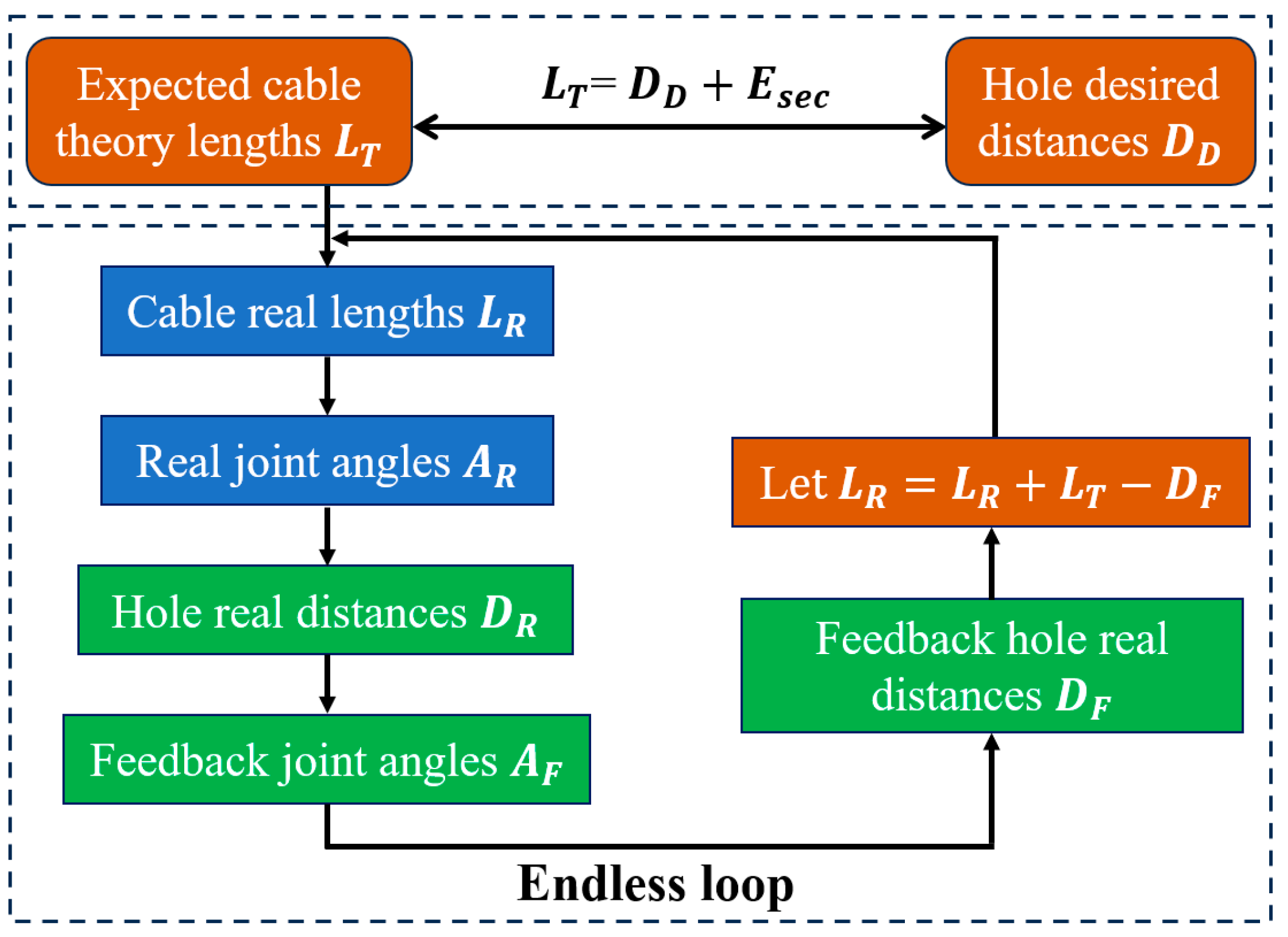
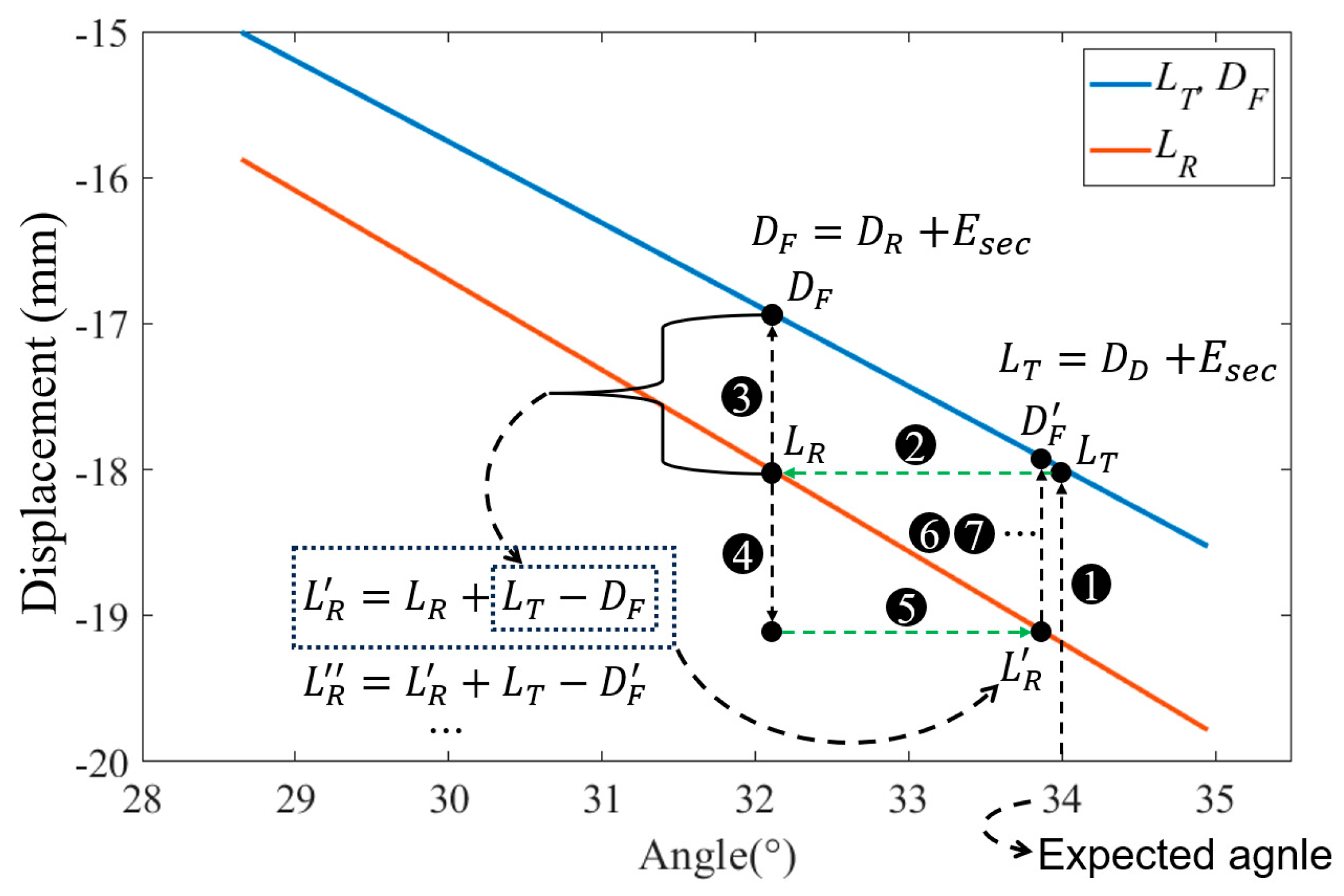
5.2. Practicability of Dual-Loop Control

For convenience, we only discuss the case with one single joint. Nevertheless, the cases with multiple joints can be analogized.

Hole zero distance (HZD) refers to the distance between the two corresponding cable holes when the arm of CSR stays straight and horizontal. HZD is obtained without considering the model error, especially the ${\mathit{E}}_{\mathit{s}\mathit{e}\mathit{c}}$. For one single joint, zero distance is equal to $2d$.

Hole real distances, ${\mathit{D}}_{\mathit{R}}$, refer to the differences in the real distances between the two groups of corresponding cable holes relative to the HZDs after the joints rotate to the certain angles. The real joint angles and model size determine ${\mathit{D}}_{\mathit{R}}$. We can calculate the feedback hole real distances, ${\mathit{D}}_{\mathit{F}}$, according to the feedback joint angles ${\mathit{A}}_{\mathit{F}}$. ${\mathit{D}}_{\mathit{F}},{\mathit{D}}_{\mathit{R}}$ are positively correlated and the main errors of ${\mathit{D}}_{\mathit{F}}$ come from ${\mathit{E}}_{\mathit{s}\mathit{e}\mathit{c}}$.

Hole desired distances, ${\mathit{D}}_{\mathit{D}}$, refer to the differences in the desired distances between the two groups of corresponding cable holes relative to the HZDs when the joints rotate to the desired angles. ${\mathit{D}}_{\mathit{D}},{\mathit{L}}_{\mathit{T}}$ are positively correlated. The main errors of ${\mathit{L}}_{\mathit{T}}$ relative to ${\mathit{D}}_{\mathit{D}}$ also come from ${\mathit{E}}_{\mathit{s}\mathit{e}\mathit{c}}$. When ${{\mathit{D}}_{\mathit{D}}=\mathit{D}}_{\mathit{R}}$, the real joint angles ${\mathit{A}}_{\mathit{R}}$ is equal to the expected joint angles ${\mathit{A}}_{\mathit{D}}$.

The essence of the driving of the joints is by changing the distances of the corresponding cable holes, which is achieved by shifting the cables. After analysis, it can be concluded that the combined effects of the first three types of errors will not cause serious deviations of ${{{\mathit{L}}_{\mathit{T}},\mathit{L}}_{\mathit{R}},{\mathit{D}}_{\mathit{D}},{\mathit{D}}_{\mathit{F}},\mathit{D}}_{\mathit{R}}$, and their varying trends are consistent. After further verification, we can know that ${{{\mathit{L}}_{\mathit{T}},\mathit{L}}_{\mathit{R}},{\mathit{D}}_{\mathit{D}},{\mathit{D}}_{\mathit{F}},\mathit{D}}_{\mathit{R}}$ are positively correlated, i.e., all increase when one increases and all decrease when one decreases. Therefore, the closed-loop control is practicable. As shown in Figure 7, the motors are driven by the expected ${\mathit{L}}_{\mathit{T}}$. That means ${\mathit{L}}_{\mathit{T}}$ will be taken as ${\mathit{L}}_{\mathit{R}}$. Then, ${\mathit{L}}_{\mathit{R}}$ will determine the real joint angles ${\mathit{A}}_{\mathit{R}}$. Thus, according to the feedback joint angles ${\mathit{A}}_{\mathit{F}}$, ${\mathit{D}}_{\mathit{F}}$ can be inversely solved. Because of the positive correlation of various variables, ${\mathit{D}}_{\mathit{R}}$ will gradually approach ${\mathit{D}}_{\mathit{D}}$ by the iteration setting of ${{\mathit{L}}_{\mathit{R}}={\mathit{L}}_{\mathit{R}}+\mathit{L}}_{\mathit{T}}-{\mathit{D}}_{\mathit{F}}$ (the real process would be more complex, such as the setting of PID parameters). In this way, not only can the complex calculation of the driving displacements of the motors be simplified, but also the effective and reliable closed-loop control can be promised.

As shown in Figure 8, the process of the closed-loop is demonstrated by taking one cable’s driving for $\mathrm{J}\mathrm{o}\mathrm{i}\mathrm{n}{\mathrm{t}}_{\mathrm{i}}$ as an example. The relations between $L_T,D_F$ and joint angle can be expressed by the same curve. The relation between $L_R$ and joint angle can be expressed by another curve. The steps in the figure have been numbered, which are explained as follows:

(1)

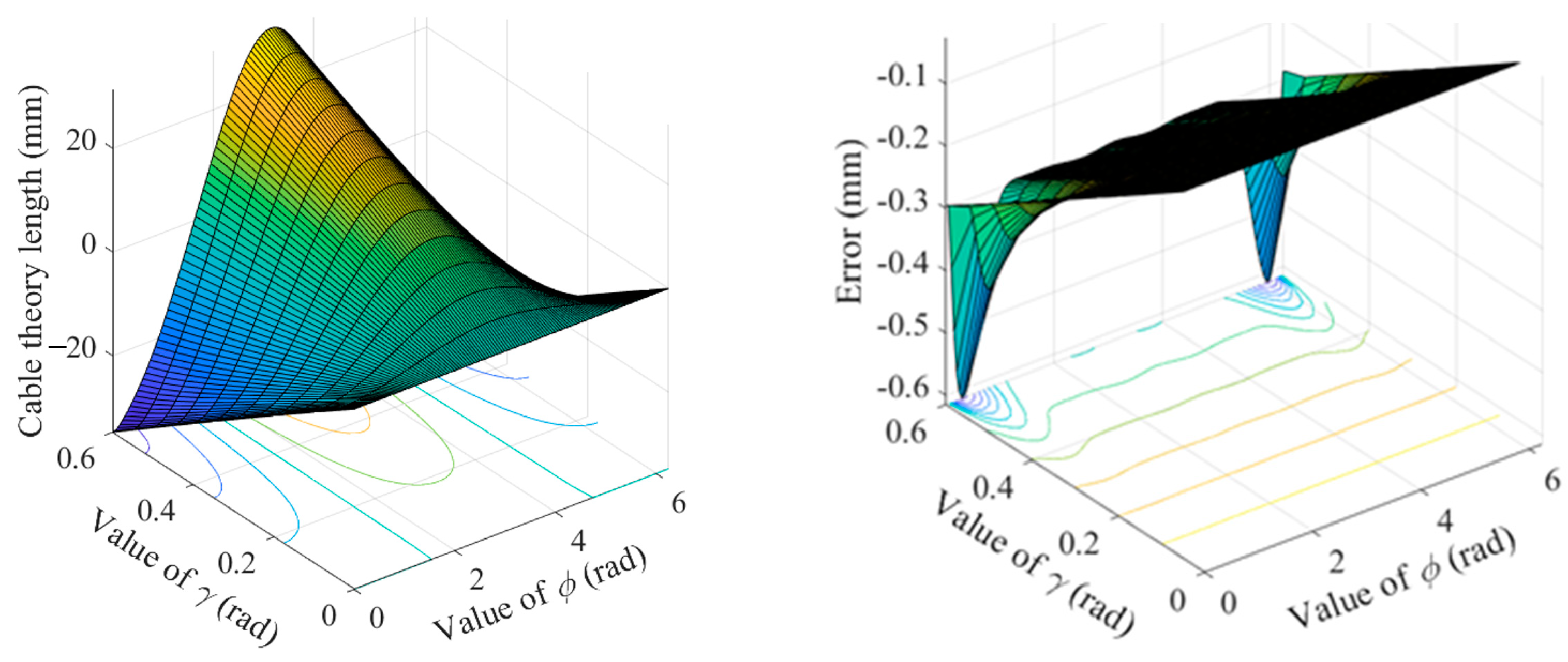
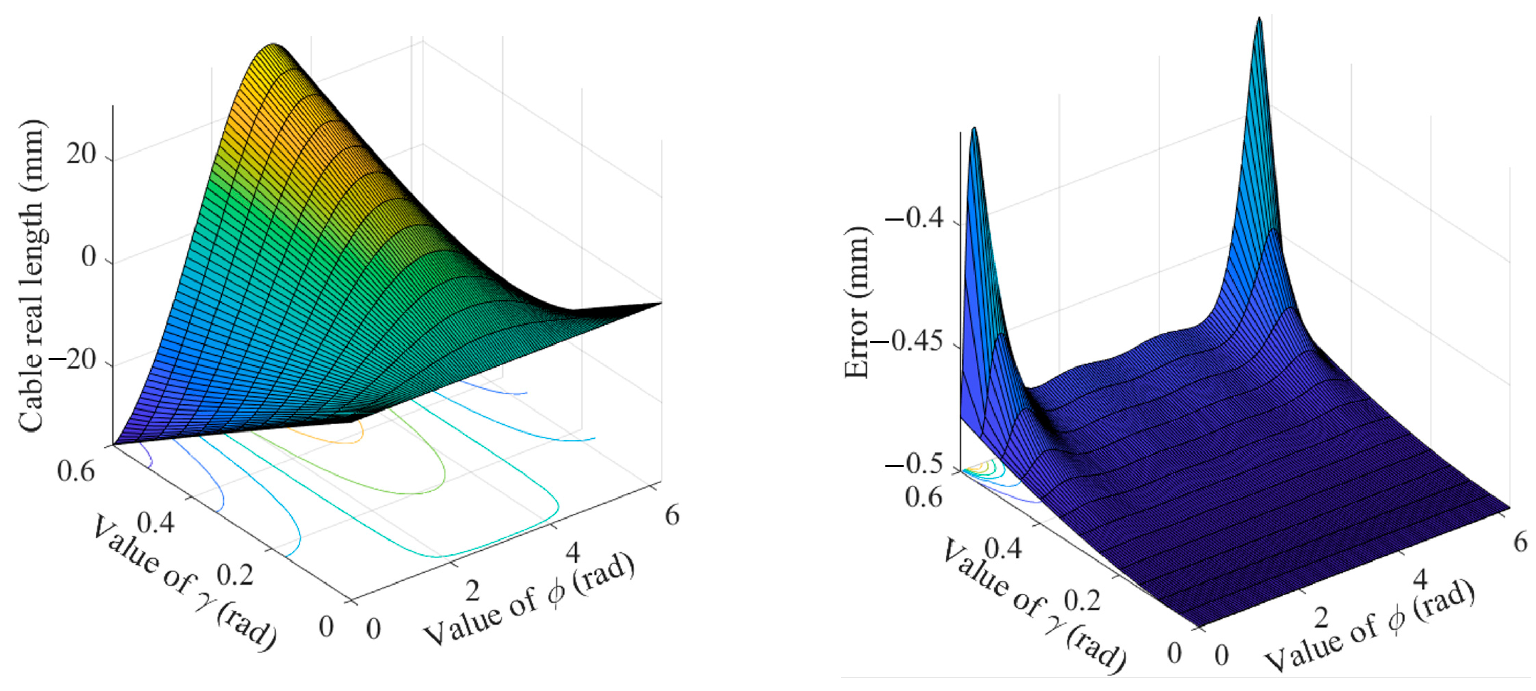
According to the expected joint angle, the expected cable theory length $L_T$ is calculated. $L_T$ will be taken as cable real length $L_R$ and input into the CSR’s driving system.

(2)

According to $L_R$, the motor moves to drive the joint.

(3)

According to the feedback joint angle $A_F$, the feedback hole real distance $D_F$ is calculated.

(4)

According to $D_F$, $L_R$ is updated to $L_R^{\prime }$.

(5)

According to the updated $L_R^{\prime }$, the motor moves to drive the joint.

(6)

and (7) $\dots$ The steps from (3) to (5) are executed in an endless loop.

Moreover, the practicability of closed-loop control can be understood more simply from the driving mode of the universal joints. Obviously, if a joint angle sensor detects the angle error, the error could be reduced by shifting the cable to make the joint rotate reversely. And the way of how to rotate the joint in reverse is exactly let ${{\mathit{L}}_{\mathit{R}}={\mathit{L}}_{\mathit{R}}+\mathit{L}}_{\mathit{T}}-{\mathit{D}}_{\mathit{F}}$.

However, $\mathrm{J}\mathrm{o}\mathrm{i}\mathrm{n}{\mathrm{t}}_{\mathrm{i}}$ would be driven by the other two cables together and their closed-loop processes are the same (Figure 8). The specific error values of the three cables would not happen to be consistent, i.e., the three cable real lengths correspond to different joint angles. The collaborative action of the three cables would obtain another real joint angle. Hence, although the closed-loop can still be carried out, the errors would accumulate with the continuous movement. As a result, the excessive errors of the cable forces would make the cables too loose and result in certain errors in the joint angles. Because of that, the feedforward control based on the feedback of the cable forces has been added to the control strategy to keep the cables tensioned and ensure the working of the closed-loop. Thus, the reliability and the accuracy of the system are promised.

5.3. Dual-Loop Control Strategy

As shown in Figure 9, the dual-loop control strategy has two loops. The force-loop processes the feedback driving forces and is to ensure the proper forces of the cables during the motion of the CSR. That not only ensures the stiffness of the robot, but also the working of the pose-loop. The pose-loop processes the feedback joint angles and achieves the closed-loop control of the robot pose, to improve the motion accuracy of the robot.

The variables and the elements in the figure are explained as follows:

The variables related to joint angles are 12-dimensional vectors, such as ${\mathit{A}}_{\mathit{D}},{\mathit{A}}_{\mathit{R}}$. The variables related to cables are 18-dimensional vectors, such as ${\mathit{L}}_{\mathit{T}},{\mathit{D}}_{\mathit{F}},{\mathit{T}}_{\mathit{F}},{\mathit{e}}_{\mathbf{1}},{\mathit{e}}_{\mathbf{2}}$. ${\mathit{T}}_{\mathit{F}}$ refers to the feedback driving forces of the cables, ${\mathit{e}}_{\mathbf{1}}$ refers to the errors calculated by the force controller, ${\mathit{e}}_{\mathbf{2}}$ refers to the errors calculated by the position controller.

“Drivers” are responsible for the driving of the DC motors, which are embedded with the position and speed-current closed-loop control algorithms.

“Time delay” refers to the inevitable delay when sensors collect data.

The “force controller” and “position controller” are both PD controllers. Their derivative elements can weaken the effects of the time delay. Their proportional and derivative gains are $K_{PF},K_{DF},K_{PP},K_{DP}$, respectively, whose value is shown in

Table 1. Parameters of all controllers.

Controller Name	Property	Value
Force controller	$K_{PF}$ (mm/N)	1.67 × 10−5
	$K_{DF}$ (mm/N)	0.5
	$\left|{\mathit{e}}_{\mathbf{1}}\right|$ (mm)	Within 0.02
Position controller	$K_{PP}$	0.04
	$K_{DP}$	0.5
	${|\mathit{e}}_{\mathbf{2}}|$ (mm)	Within 0.02
PID controller	Value of ${\mathit{K}}_{\mathit{P}\mathit{A}}$’s element	0.5–1.5
	Value of ${\mathit{K}}_{\mathit{D}\mathit{A}}$’s element	0.1–0.5
	Value of ${\mathit{K}}_{\mathit{I}\mathit{A}}$’s element	0.1–0.3
	$\rho$	0.01

. Additionally, to avoid the excessive overshoot, both ${\mathit{e}}_{\mathbf{1}},{\mathit{e}}_{\mathbf{2}}$ have been set within borders.

Let $∆\mathit{T}\left(j\right)={\mathit{T}}_{\mathit{F}}\left(j\right)-{\mathit{T}}_{\mathit{T}}\left(j\right)$ (${\mathit{T}}_{\mathit{T}}$ refer to the values of the driving forces of the cables, which are calculated through the inverse dynamics), then the value of $j$th component in ${\mathit{e}}_{\mathbf{1}}$ is

$${\mathit{e}}_{\mathbf{1}}\left(j\right)=\left\{\begin{array}{c}0.02if{\mathit{e}}_{\mathbf{1}}\left(j\right)>0.02\\ -0.02if{\mathit{e}}_{\mathbf{1}}\left(j\right)<-0.02\\ K_{PF}∆\mathit{T}\left(j\right)+K_{DF}[∆\mathit{T}(j)-∆{\mathit{T}}^{\prime }(j\left)\right]\end{array}\right.$$

(29)

$∆{\mathit{T}}^{\prime }$: value of $∆\mathit{T}$ at previous period.

Let $∆\mathit{L}\left(j\right)={\mathit{L}}_{\mathit{T}}\left(j\right)-D_{\mathit{F}}\left(j\right)$, then the value of $j$th component in ${\mathit{e}}_{\mathbf{2}}$ is

$${\mathit{e}}_{\mathbf{2}}\left(j\right)=\left\{\begin{array}{c}0.02if{\mathit{e}}_{\mathbf{2}}\left(j\right)>0.02\\ -0.02if{\mathit{e}}_{\mathbf{2}}\left(j\right)<-0.02\\ K_{PP}∆\mathit{L}\left(j\right)+K_{DP}[∆\mathit{L}\left(j\right)-∆{\mathit{L}}^{\prime }\left(j\right)]\end{array}\right.$$

(30)

$∆{\mathit{L}}^{\prime }$: value of $∆\mathit{L}$ at previous period.

The “PID” controller integrates the input variables ${\mathit{e}}_{\mathbf{1}},{\mathit{e}}_{\mathbf{2}}$ to obtain the integrated errors $\mathit{E}$. And then $\mathit{E}$ are combined with the current ${\mathit{L}}_{\mathit{T}}$ to obtain the motor displacements, ${\mathit{L}}_{\mathit{s}}$, which is required by the drivers. As the cables have various load characteristics and lengths, the PID parameters are different for each cable, as shown in Table 1. Moreover, because the regular integrator element would result in the instability of the system, i.e., causing too large or small cable forces, the weighting factor is added for the integrator element to weaken the influence of historical errors. Thus, the stability of the system can be improved. Let

$${\mathit{e}}_{\mathit{s}}={\mathit{e}}_{\mathbf{1}}+{\mathit{e}}_{\mathbf{2}}$$

(31)

Then, the elements of $\mathit{E}$ can be calculated by the following two equations (take ${\mathrm{C}}_{\mathrm{j}}$ as an example again),

$$\mathit{E}\left(j\right)={\mathit{K}}_{\mathit{P}\mathit{A}}^{}\left(j\right){\mathit{e}}_{\mathit{s}}\left(j\right)+{\mathit{K}}_{\mathit{D}\mathit{A}}^{}\left(j\right)∆{\mathit{e}}_{\mathit{s}}+{\mathit{K}}_{\mathit{I}\mathit{A}}^{}\left(j\right){\mathit{S}}_{\mathit{E}}^{\prime }\left(j\right)$$

(32)

$${\mathit{S}}_{\mathit{E}}=\mathit{E}+\rho {\mathit{S}}_{\mathit{E}}^{\prime }$$

(33)

$∆{\mathit{e}}_{\mathit{s}}$: difference between current ${\mathit{e}}_{\mathit{s}}$ and last ${\mathit{e}}_{\mathit{s}}$.

${\mathit{S}}_{\mathit{E}}$: sum of historical weighted $\mathit{E}$.

${\mathit{S}}_{\mathit{E}}^{\prime }$: value of ${\mathit{S}}_{\mathit{E}}$ at previous period.

Then, the motor displacements ${\mathit{L}}_{\mathit{s}}$ are

$${\mathit{L}}_{\mathit{s}}={\mathit{L}}_{\mathit{T}}+\mathit{E}$$

(34)

Thus, the CSR’s dual-loop controller has been designed.

6. Experimental Results and Discussion

To substantiate the effectiveness and reliability of the proposed dual-loop control strategy, a series of experiments have been presented on a CSR prototype. To illustrate the superiority of the proposed method, the CSR prototype not only has run the dual-loop mode motion test, but also the comparison experiments, i.e., the open-loop and single-loop (pose-loop) modes tests. According to the material property, the coulomb friction coefficient has been set as $\mu =0.14$. The experiments can be divided into three parts, single joint test, multiple joints test, and continuous motion test.

6.1. Single Joint Test

Single joint test refers to rotating a single joint of the CSR and then comparing the difference among the feedback joint angles.

Table 2. Single joint test of $\mathrm{J}\mathrm{o}\mathrm{i}\mathrm{n}{\mathrm{t}}_6$.

Reference Angles	Feedback Angles
	Open-Loop	Single-Loop	Dual-Loop
$\left[\begin{array}{c}\begin{array}{c}{\mathsf{\alpha }}_1\hspace{1em}{\mathsf{\beta }}_1\\ {\mathsf{\alpha }}_2\hspace{1em}{\mathsf{\beta }}_2\\ {\mathsf{\alpha }}_3\hspace{1em}{\mathsf{\beta }}_3\end{array}\\ {\mathsf{\alpha }}_4\hspace{1em}{\mathsf{\beta }}_4\\ \begin{array}{c}{\mathsf{\alpha }}_5\hspace{1em}{\mathsf{\beta }}_5\\ {\mathsf{\alpha }}_6\hspace{1em}{\mathsf{\beta }}_6\end{array}\end{array}\right]=\left[\begin{array}{c}\begin{array}{c}0°\hspace{1em}0°\\ 0°\hspace{1em}0°\\ 0°\hspace{1em}0°\end{array}\\ 0°\hspace{1em}0°\\ \begin{array}{c}0°\hspace{1em}0°\\ 10°\hspace{1em}0°\end{array}\end{array}\right]$	$\left[\begin{array}{c}\begin{array}{c}-0.101°\hspace{1em}0.066°\\ 0.051°\hspace{1em}-0.074°\\ 0.000°\hspace{1em}-0.055°\end{array}\\ -0.021°\hspace{1em}0.138°\\ \begin{array}{c}0.006°\hspace{1em}-0.085°\\ 10.261°\hspace{1em}0.143°\end{array}\end{array}\right]$	$\left[\begin{array}{c}\begin{array}{c}0.261°\hspace{1em}0.011°\\ -0.377°\hspace{1em}-0.139°\\ -0.055°\hspace{1em}0.181°\end{array}\\ 0.221°\hspace{1em}-0.137°\\ \begin{array}{c}0.094°\hspace{1em}0.069°\\ 9.921°\hspace{1em}-0.033°\end{array}\end{array}\right]$	$\left[\begin{array}{c}\begin{array}{c}0.011°\hspace{1em}-0.003°\\ -0.016°\hspace{1em}-0.081°\\ 0.014°\hspace{1em}0.066°\end{array}\\ 0.006°\hspace{1em}0.023°\\ \begin{array}{c}0.003°\hspace{1em}-0.016°\\ 10.009°\hspace{1em}0.000°\end{array}\end{array}\right]$
$\left[\begin{array}{c}\begin{array}{c}{\mathsf{\alpha }}_1\hspace{1em}{\mathsf{\beta }}_1\\ {\mathsf{\alpha }}_2\hspace{1em}{\mathsf{\beta }}_2\\ {\mathsf{\alpha }}_3\hspace{1em}{\mathsf{\beta }}_3\end{array}\\ {\mathsf{\alpha }}_4\hspace{1em}{\mathsf{\beta }}_4\\ \begin{array}{c}{\mathsf{\alpha }}_5\hspace{1em}{\mathsf{\beta }}_5\\ {\mathsf{\alpha }}_6\hspace{1em}{\mathsf{\beta }}_6\end{array}\end{array}\right]=\left[\begin{array}{c}\begin{array}{c}0°\hspace{1em}0°\\ 0°\hspace{1em}0°\\ 0°\hspace{1em}0°\end{array}\\ 0°\hspace{1em}0°\\ \begin{array}{c}0°\hspace{1em}0°\\ 20°\hspace{1em}0°\end{array}\end{array}\right]$	$\left[\begin{array}{c}\begin{array}{c}-0.112°\hspace{1em}0.077°\\ 0.062°\hspace{1em}-0.096°\\ 0.011°\hspace{1em}-0.066°\end{array}\\ -0.021°\hspace{1em}0.138°\\ \begin{array}{c}0.006°\hspace{1em}-0.096°\\ 20.500°\hspace{1em}0.198°\end{array}\end{array}\right]$	$\left[\begin{array}{c}\begin{array}{c}0.261°\hspace{1em}0.000°\\ -0.399°\hspace{1em}-0.128°\\ -0.055°\hspace{1em}0.181°\end{array}\\ 0.221°\hspace{1em}-0.126°\\ \begin{array}{c}0.094°\hspace{1em}0.080°\\ 20.204°\hspace{1em}-0.022°\end{array}\end{array}\right]$	$\left[\begin{array}{c}\begin{array}{c}0.000°\hspace{1em}0.008°\\ -0.016°\hspace{1em}-0.081°\\ 0.013°\hspace{1em}0.088°\end{array}\\ 0.006°\hspace{1em}-0.001°\\ \begin{array}{c}-0.008°\hspace{1em}0.006°\\ 20.017°\hspace{1em}0.011°\end{array}\end{array}\right]$
$\left[\begin{array}{c}\begin{array}{c}{\mathsf{\alpha }}_1\hspace{1em}{\mathsf{\beta }}_1\\ {\mathsf{\alpha }}_2\hspace{1em}{\mathsf{\beta }}_2\\ {\mathsf{\alpha }}_3\hspace{1em}{\mathsf{\beta }}_3\end{array}\\ {\mathsf{\alpha }}_4\hspace{1em}{\mathsf{\beta }}_4\\ \begin{array}{c}{\mathsf{\alpha }}_5\hspace{1em}{\mathsf{\beta }}_5\\ {\mathsf{\alpha }}_6\hspace{1em}{\mathsf{\beta }}_6\end{array}\end{array}\right]=\left[\begin{array}{c}\begin{array}{c}0°\hspace{1em}0°\\ 0°\hspace{1em}0°\\ 0°\hspace{1em}0°\end{array}\\ 0°\hspace{1em}0°\\ \begin{array}{c}0°\hspace{1em}0°\\ 30°\hspace{1em}0°\end{array}\end{array}\right]$	$\left[\begin{array}{c}\begin{array}{c}-0.112°\hspace{1em}0.055°\\ 0.073°\hspace{1em}-0.074°\\ 0.011°\hspace{1em}-0.055°\end{array}\\ -0.021°\hspace{1em}0.127°\\ \begin{array}{c}-0.005°\hspace{1em}-0.096°\\ 30.762°\hspace{1em}0.231°\end{array}\end{array}\right]$	$\left[\begin{array}{c}\begin{array}{c}0.261°\hspace{1em}0.000°\\ -0.388°\hspace{1em}-0.128°\\ -0.055°\hspace{1em}0.170°\end{array}\\ 0.210°\hspace{1em}-0.126°\\ \begin{array}{c}0.094°\hspace{1em}0.080°\\ 30.432°\hspace{1em}-0.011°\end{array}\end{array}\right]$	$\left[\begin{array}{c}\begin{array}{c}0.000°\hspace{1em}-0.003°\\ -0.016°\hspace{1em}-0.081°\\ 0.014°\hspace{1em}0.088°\end{array}\\ 0.006°\hspace{1em}0.001°\\ \begin{array}{c}0.003°\hspace{1em}-0.016°\\ 30.004°\hspace{1em}0.000°\end{array}\end{array}\right]$

shows the test data of ${\mathsf{\alpha }}_6$. Because of the nonlinear coupling relations among the cables and the universal joints, the other joint angles would be influenced even if we changed only one joint angle. Thus, the recording data are not limited to ${\mathsf{\alpha }}_6$, but also are with ${\mathsf{\alpha }}_1,{\mathsf{\alpha }}_2,\dots {\mathsf{\alpha }}_5,{\beta }_1, {\beta }_2,\dots {\mathsf{\beta }}_6$. Moreover, the other joints have also been tested with various joint angles. However, since the results of different joints tests are similar, we have not listed them one by one.

The single joint test results show that the steady-state accuracy of the dual-loop control mode has been significantly improved. The accuracy of the single-loop mode is slightly improved compared to the open-loop. Furthermore, it can be found that the smaller the joint rotation angle, the higher the accuracy of the single-loop.

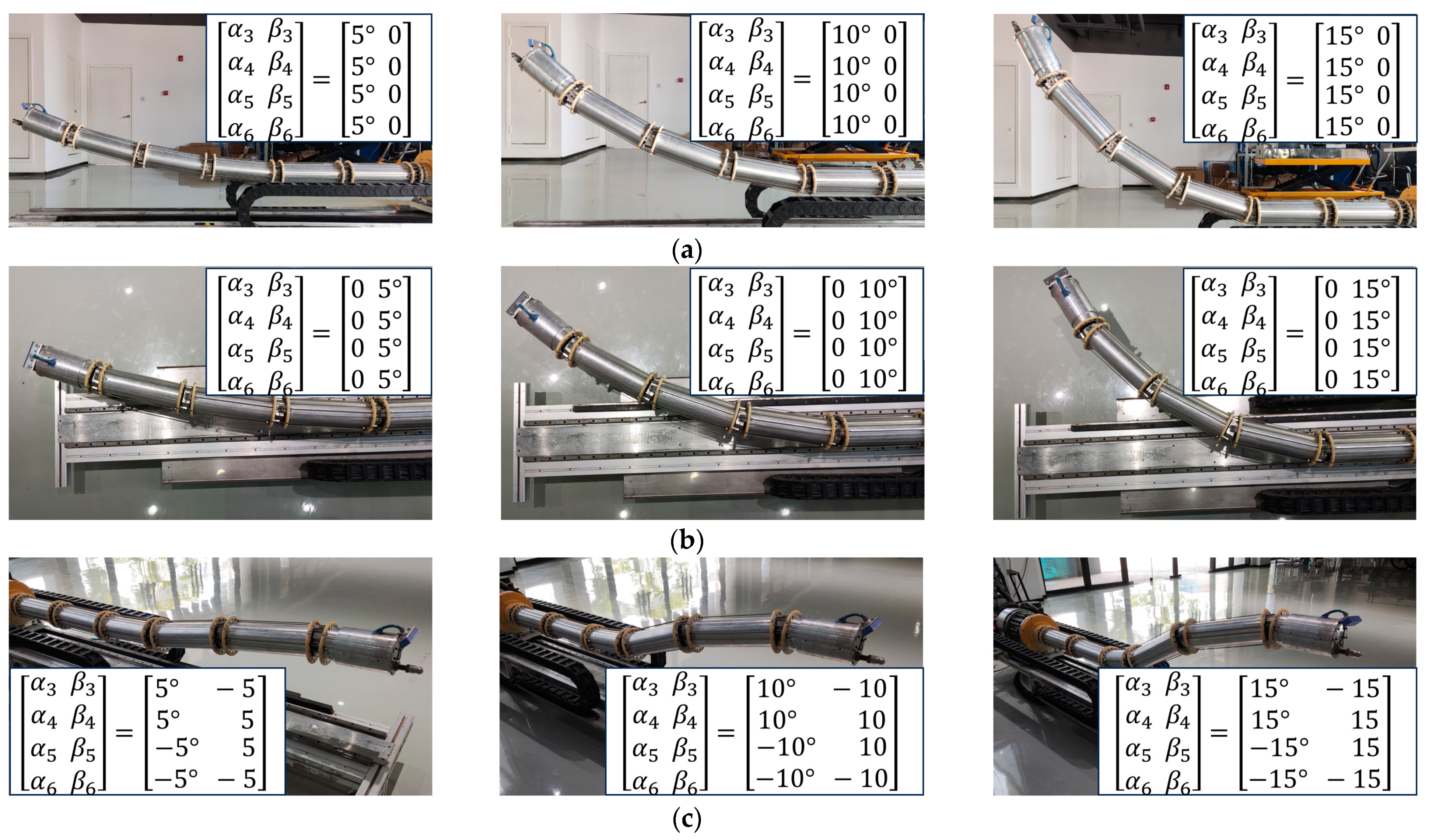
6.2. Multiple Joints Test

The multiple joints test refers to rotating multiple joints of the CSR and then comparing the difference among the feedback joint angles.

Table 3. Multiple pitch joints test.

Reference Angles	Feedback Angles
	Open-Loop	Single-Loop	Dual-Loop
$\left[\begin{array}{c}\begin{array}{c}{\mathsf{\alpha }}_1\hspace{1em}{\mathsf{\beta }}_1\\ {\mathsf{\alpha }}_2\hspace{1em}{\mathsf{\beta }}_2\\ {\mathsf{\alpha }}_3\hspace{1em}{\mathsf{\beta }}_3\end{array}\\ {\mathsf{\alpha }}_4\hspace{1em}{\mathsf{\beta }}_4\\ \begin{array}{c}{\mathsf{\alpha }}_5\hspace{1em}{\mathsf{\beta }}_5\\ {\mathsf{\alpha }}_6\hspace{1em}{\mathsf{\beta }}_6\end{array}\end{array}\right]=\left[\begin{array}{c}\begin{array}{c}0°\hspace{1em}0°\\ 0°\hspace{1em}0°\\ 5°\hspace{1em}0°\end{array}\\ 5°\hspace{1em}0°\\ \begin{array}{c}5°\hspace{1em}0°\\ 5°\hspace{1em}0°\end{array}\end{array}\right]$	$\left[\begin{array}{c}\begin{array}{c}-0.189°\hspace{1em}0.022°\\ 0.941°\hspace{1em}0.014°\\ 4.296°\hspace{1em}0.016°\end{array}\\ 5.351°\hspace{1em}0.050°\\ \begin{array}{c}4.994°\hspace{1em}-0.041°\\ 5.197°\hspace{1em}-0.033°\end{array}\end{array}\right]$	$\left[\begin{array}{c}\begin{array}{c}-0.288°\hspace{1em}0.011°\\ 0.469°\hspace{1em}0.003°\\ 4.296°\hspace{1em}0.115°\end{array}\\ 5.186°\hspace{1em}-0.104°\\ \begin{array}{c}5.664°\hspace{1em}-0.118°\\ 4.570°\hspace{1em}-0.154°\end{array}\end{array}\right]$	$\left[\begin{array}{c}\begin{array}{c}-0.014°\hspace{1em}0.000°\\ 0.018°\hspace{1em}0.003°\\ 4.999°\hspace{1em}-0.006°\end{array}\\ 5.000°\hspace{1em}0.006°\\ \begin{array}{c}5.005°\hspace{1em}-0.008°\\ 4.999°\hspace{1em}0.000°\end{array}\end{array}\right]$
$\left[\begin{array}{c}\begin{array}{c}{\mathsf{\alpha }}_1\hspace{1em}{\mathsf{\beta }}_1\\ {\mathsf{\alpha }}_2\hspace{1em}{\mathsf{\beta }}_2\\ {\mathsf{\alpha }}_3\hspace{1em}{\mathsf{\beta }}_3\end{array}\\ {\mathsf{\alpha }}_4\hspace{1em}{\mathsf{\beta }}_4\\ \begin{array}{c}{\mathsf{\alpha }}_5\hspace{1em}{\mathsf{\beta }}_5\\ {\mathsf{\alpha }}_6\hspace{1em}{\mathsf{\beta }}_6\end{array}\end{array}\right]=\left[\begin{array}{c}\begin{array}{c}0°\hspace{1em}0°\\ 0°\hspace{1em}0°\\ 10°\hspace{1em}0°\end{array}\\ 10°\hspace{1em}0°\\ \begin{array}{c}10°\hspace{1em}0°\\ 10°\hspace{1em}0°\end{array}\end{array}\right]$	$\left[\begin{array}{c}\begin{array}{c}-0.200°\hspace{1em}0.011°\\ 0.941°\hspace{1em}0.003°\\ 9.503°\hspace{1em}0.016°\end{array}\\ 10.427°\hspace{1em}0.028°\\ \begin{array}{c}10.157°\hspace{1em}-0.030°\\ 10.162°\hspace{1em}-0.022°\end{array}\end{array}\right]$	$\left[\begin{array}{c}\begin{array}{c}-0.277°\hspace{1em}0.022°\\ 0.469°\hspace{1em}0.003°\\ 10.349°\hspace{1em}0.115°\end{array}\\ 9.702°\hspace{1em}-0.115°\\ \begin{array}{c}10.883°\hspace{1em}-0.140°\\ 9.470°\hspace{1em}0.209°\end{array}\end{array}\right]$	$\left[\begin{array}{c}\begin{array}{c}-0.003°\hspace{1em}0.000°\\ 0.007°\hspace{1em}-0.008°\\ 9.987°\hspace{1em}-0.006°\end{array}\\ 9.988°\hspace{1em}-0.016°\\ \begin{array}{c}10.004°\hspace{1em}-0.008°\\ 9.998°\hspace{1em}0.000°\end{array}\end{array}\right]$
$\left[\begin{array}{c}\begin{array}{c}{\mathsf{\alpha }}_1\hspace{1em}{\mathsf{\beta }}_1\\ {\mathsf{\alpha }}_2\hspace{1em}{\mathsf{\beta }}_2\\ {\mathsf{\alpha }}_3\hspace{1em}{\mathsf{\beta }}_3\end{array}\\ {\mathsf{\alpha }}_4\hspace{1em}{\mathsf{\beta }}_4\\ \begin{array}{c}{\mathsf{\alpha }}_5\hspace{1em}{\mathsf{\beta }}_5\\ {\mathsf{\alpha }}_6\hspace{1em}{\mathsf{\beta }}_6\end{array}\end{array}\right]=\left[\begin{array}{c}\begin{array}{c}0°\hspace{1em}0°\\ 0°\hspace{1em}0°\\ 15°\hspace{1em}0°\end{array}\\ 15°\hspace{1em}0°\\ \begin{array}{c}15°\hspace{1em}0°\\ 15°\hspace{1em}0°\end{array}\end{array}\right]$	$\left[\begin{array}{c}\begin{array}{c}-0.200°\hspace{1em}0.022°\\ 0.919°\hspace{1em}0.003°\\ 14.667°\hspace{1em}0.005°\end{array}\\ 15.547°\hspace{1em}0.017°\\ \begin{array}{c}15.431°\hspace{1em}-0.041°\\ 15.106°\hspace{1em}-0.033°\end{array}\end{array}\right]$	$\left[\begin{array}{c}\begin{array}{c}-0.310°\hspace{1em}0.011°\\ 0.469°\hspace{1em}0.003°\\ 15.524°\hspace{1em}0.115°\end{array}\\ 14.800°\hspace{1em}-0.093°\\ \begin{array}{c}16.222°\hspace{1em}-0.250°\\ 14.392°\hspace{1em}0.319°\end{array}\end{array}\right]$	$\left[\begin{array}{c}\begin{array}{c}-0.003°\hspace{1em}0.011°\\ -0.015°\hspace{1em}0.003°\\ 14.996°\hspace{1em}-0.005°\end{array}\\ 15.008°\hspace{1em}0.006°\\ \begin{array}{c}15.002°\hspace{1em}-0.003°\\ 15.007°\hspace{1em}0.011°\end{array}\end{array}\right]$

presents the data of the multiple pitch joints test, i.e., ${\mathsf{\alpha }}_3,{\mathsf{\alpha }}_4,{\mathsf{\alpha }}_5,{\mathsf{\alpha }}_6$.

Table 4. Multiple yaw joints test.

Reference Angles	Feedback Angles
	Open-Loop	Single-Loop	Dual-Loop
$\left[\begin{array}{c}\begin{array}{c}{\mathsf{\alpha }}_1\hspace{1em}{\mathsf{\beta }}_1\\ {\mathsf{\alpha }}_2\hspace{1em}{\mathsf{\beta }}_2\\ {\mathsf{\alpha }}_3\hspace{1em}{\mathsf{\beta }}_3\end{array}\\ {\mathsf{\alpha }}_4\hspace{1em}{\mathsf{\beta }}_4\\ \begin{array}{c}{\mathsf{\alpha }}_5\hspace{1em}{\mathsf{\beta }}_5\\ {\mathsf{\alpha }}_6\hspace{1em}{\mathsf{\beta }}_6\end{array}\end{array}\right]=\left[\begin{array}{c}\begin{array}{c}0°\hspace{1em}0°\\ 0°\hspace{1em}0°\\ 0°\hspace{1em}5°\end{array}\\ 0°\hspace{1em}5°\\ \begin{array}{c}0°\hspace{1em}5°\\ 0°\hspace{1em}5°\end{array}\end{array}\right]$	$\left[\begin{array}{c}\begin{array}{c}0.063°\hspace{1em}-0.011°\\ -0.092°\hspace{1em}0.003°\\ -0.077°\hspace{1em}5.103°\end{array}\\ 0.056°\hspace{1em}4.686°\\ \begin{array}{c}0.061°\hspace{1em}5.441°\\ -0.066°\hspace{1em}4.790°\end{array}\end{array}\right]$	$\left[\begin{array}{c}\begin{array}{c}0.272°\hspace{1em}-0.044°\\ -0.619°\hspace{1em}0.102°\\ 0.363°\hspace{1em}4.916°\end{array}\\ -0.021°\hspace{1em}4.807°\\ \begin{array}{c}0.039°\hspace{1em}5.496°\\ -0.121°\hspace{1em}4.636°\end{array}\end{array}\right]$	$\left[\begin{array}{c}\begin{array}{c}-0.046°\hspace{1em}0.033°\\ 0.025°\hspace{1em}0.025°\\ 0.011°\hspace{1em}5.004°\end{array}\\ -0.010°\hspace{1em}5.005°\\ \begin{array}{c}-0.005°\hspace{1em}4.991°\\ 0.000°\hspace{1em}4.999°\end{array}\end{array}\right]$
$\left[\begin{array}{c}\begin{array}{c}{\mathsf{\alpha }}_1\hspace{1em}{\mathsf{\beta }}_1\\ {\mathsf{\alpha }}_2\hspace{1em}{\mathsf{\beta }}_2\\ {\mathsf{\alpha }}_3\hspace{1em}{\mathsf{\beta }}_3\end{array}\\ {\mathsf{\alpha }}_4\hspace{1em}{\mathsf{\beta }}_4\\ \begin{array}{c}{\mathsf{\alpha }}_5\hspace{1em}{\mathsf{\beta }}_5\\ {\mathsf{\alpha }}_6\hspace{1em}{\mathsf{\beta }}_6\end{array}\end{array}\right]=\left[\begin{array}{c}\begin{array}{c}0°\hspace{1em}0°\\ 0°\hspace{1em}0°\\ 0°\hspace{1em}10°\end{array}\\ 0°\hspace{1em}10°\\ \begin{array}{c}0°\hspace{1em}10°\\ 0°\hspace{1em}10°\end{array}\end{array}\right]$	$\left[\begin{array}{c}\begin{array}{c}0.140°\hspace{1em}-0.022°\\ -0.081°\hspace{1em}-0.041°\\ -0.088°\hspace{1em}10.277°\end{array}\\ 0.045°\hspace{1em}9.531°\\ \begin{array}{c}0.039°\hspace{1em}10.451°\\ -0.077°\hspace{1em}9.756°\end{array}\end{array}\right]$	$\left[\begin{array}{c}\begin{array}{c}0.294°\hspace{1em}-0.077°\\ -0.608°\hspace{1em}0.069°\\ 0.385°\hspace{1em}10.101°\end{array}\\ -0.131°\hspace{1em}9.652°\\ \begin{array}{c}0.028°\hspace{1em}10.517°\\ -0.088°\hspace{1em}9.580°\end{array}\end{array}\right]$	$\left[\begin{array}{c}\begin{array}{c}-0.046°\hspace{1em}0.033°\\ 0.040°\hspace{1em}0.025°\\ 0.000°\hspace{1em}9.992°\end{array}\\ 0.001°\hspace{1em}10.015°\\ \begin{array}{c}-0.005°\hspace{1em}10.001°\\ 0.000°\hspace{1em}10.009°\end{array}\end{array}\right]$
$\left[\begin{array}{c}\begin{array}{c}{\mathsf{\alpha }}_1\hspace{1em}{\mathsf{\beta }}_1\\ {\mathsf{\alpha }}_2\hspace{1em}{\mathsf{\beta }}_2\\ {\mathsf{\alpha }}_3\hspace{1em}{\mathsf{\beta }}_3\end{array}\\ {\mathsf{\alpha }}_4\hspace{1em}{\mathsf{\beta }}_4\\ \begin{array}{c}{\mathsf{\alpha }}_5\hspace{1em}{\mathsf{\beta }}_5\\ {\mathsf{\alpha }}_6\hspace{1em}{\mathsf{\beta }}_6\end{array}\end{array}\right]=\left[\begin{array}{c}\begin{array}{c}0°\hspace{1em}0°\\ 0°\hspace{1em}0°\\ 0°\hspace{1em}15°\end{array}\\ 0°\hspace{1em}15°\\ \begin{array}{c}0°\hspace{1em}15°\\ 0°\hspace{1em}15°\end{array}\end{array}\right]$	$\left[\begin{array}{c}\begin{array}{c}0.206°\hspace{1em}-0.044°\\ -0.059°\hspace{1em}-0.074°\\ -0.165°\hspace{1em}15.408°\end{array}\\ 0.023°\hspace{1em}14.442°\\ \begin{array}{c}0.028°\hspace{1em}15.417°\\ -0.077°\hspace{1em}14.733°\end{array}\end{array}\right]$	$\left[\begin{array}{c}\begin{array}{c}0.316°\hspace{1em}-0.099°\\ -0.553°\hspace{1em}0.036°\\ 0.406°\hspace{1em}15.265°\end{array}\\ -0.263°\hspace{1em}14.508°\\ \begin{array}{c}0.028°\hspace{1em}15.527°\\ -0.011°\hspace{1em}14.491°\end{array}\end{array}\right]$	$\left[\begin{array}{c}\begin{array}{c}-0.046°\hspace{1em}-0.022°\\ 0.029°\hspace{1em}0.014°\\ 0.000°\hspace{1em}15.001°\end{array}\\ -0.001°\hspace{1em}15.024°\\ \begin{array}{c}0.017°\hspace{1em}14.966°\\ -0.011°\hspace{1em}15.007°\end{array}\end{array}\right]$

presents the data of the multiple yaw joints test, i.e., ${\mathsf{\beta }}_3, {\mathsf{\beta }}_4, {\mathsf{\beta }}_5, {\mathsf{\beta }}_6$.

Table 5. Multiple pitch and yaw joints test.

Reference Angles	Feedback Angles
	Open-Loop	Single-Loop	Dual-Loop
$\left[\begin{array}{c}\begin{array}{c}{\mathsf{\alpha }}_1\hspace{1em}{\mathsf{\beta }}_1\\ {\mathsf{\alpha }}_2\hspace{1em}{\mathsf{\beta }}_2\\ {\mathsf{\alpha }}_3\hspace{1em}{\mathsf{\beta }}_3\end{array}\\ {\mathsf{\alpha }}_4\hspace{1em}{\mathsf{\beta }}_4\\ \begin{array}{c}{\mathsf{\alpha }}_5\hspace{1em}{\mathsf{\beta }}_5\\ {\mathsf{\alpha }}_6\hspace{1em}{\mathsf{\beta }}_6\end{array}\end{array}\right]=\left[\begin{array}{c}\begin{array}{c}0°\hspace{1em}0°\\ 0°\hspace{1em}0°\\ 5°\hspace{1em}-5°\end{array}\\ 5°\hspace{1em}5°\\ \begin{array}{c}-5°\hspace{1em}5°\\ -5°\hspace{1em}-5°\end{array}\end{array}\right]$	$\left[\begin{array}{c}\begin{array}{c}-0.079°\hspace{1em}0.011°\\ -0.103°\hspace{1em}-0.030°\\ 5.537°\hspace{1em}-5.010°\end{array}\\ 4.879°\hspace{1em}5.565°\\ \begin{array}{c}-5.542°\hspace{1em}4.782°\\ -4.603°\hspace{1em}-5.306°\end{array}\end{array}\right]$	$\left[\begin{array}{c}\begin{array}{c}0.239°\hspace{1em}0.044°\\ -0.619°\hspace{1em}-0.392°\\ 5.702°\hspace{1em}-4.307°\end{array}\\ 4.791°\hspace{1em}4.807°\\ \begin{array}{c}-5.059°\hspace{1em}5.112°\\ -5.032°\hspace{1em}-5.240°\end{array}\end{array}\right]$	$\left[\begin{array}{c}\begin{array}{c}0.008°\hspace{1em}0.000°\\ -0.004°\hspace{1em}-0.008°\\ 4.999°\hspace{1em}-4.999°\end{array}\\ 4.978°\hspace{1em}4.994°\\ \begin{array}{c}-5.004°\hspace{1em}5.002°\\ -4.999°\hspace{1em}-5.010°\end{array}\end{array}\right]$
$\left[\begin{array}{c}\begin{array}{c}{\mathsf{\alpha }}_1\hspace{1em}{\mathsf{\beta }}_1\\ {\mathsf{\alpha }}_2\hspace{1em}{\mathsf{\beta }}_2\\ {\mathsf{\alpha }}_3\hspace{1em}{\mathsf{\beta }}_3\end{array}\\ {\mathsf{\alpha }}_4\hspace{1em}{\mathsf{\beta }}_4\\ \begin{array}{c}{\mathsf{\alpha }}_5\hspace{1em}{\mathsf{\beta }}_5\\ {\mathsf{\alpha }}_6\hspace{1em}{\mathsf{\beta }}_6\end{array}\end{array}\right]=\left[\begin{array}{c}\begin{array}{c}0°\hspace{1em}0°\\ 0°\hspace{1em}0°\\ 5°\hspace{1em}-5°\end{array}\\ 5°\hspace{1em}5°\\ \begin{array}{c}-5°\hspace{1em}5°\\ -5°\hspace{1em}-5°\end{array}\end{array}\right]$	$\left[\begin{array}{c}\begin{array}{c}-0.079°\hspace{1em}0.022°\\ -0.103°\hspace{1em}-0.030°\\ 10.613°\hspace{1em}-10.393°\end{array}\\ 10.054°\hspace{1em}10.948°\\ \begin{array}{c}-10.739°\hspace{1em}10.122°\\ -9.382°\hspace{1em}-10.723°\end{array}\end{array}\right]$	$\left[\begin{array}{c}\begin{array}{c}0.327°\hspace{1em}0.033°\\ -0.773°\hspace{1em}-0.030°\\ 10.833°\hspace{1em}-10.327°\end{array}\\ 9.988°\hspace{1em}10.784°\\ \begin{array}{c}-10.574°\hspace{1em}9.891°\\ -9.404°\hspace{1em}-10.272°\end{array}\end{array}\right]$	$\left[\begin{array}{c}\begin{array}{c}-0.003°\hspace{1em}-0.011°\\ -0.004°\hspace{1em}-0.008°\\ 9.998°\hspace{1em}-9.998°\end{array}\\ 9.988°\hspace{1em}10.004°\\ \begin{array}{c}-10.002°\hspace{1em}10.001°\\ -9.998°\hspace{1em}-9.998°\end{array}\end{array}\right]$
$\left[\begin{array}{c}\begin{array}{c}{\mathsf{\alpha }}_1\hspace{1em}{\mathsf{\beta }}_1\\ {\mathsf{\alpha }}_2\hspace{1em}{\mathsf{\beta }}_2\\ {\mathsf{\alpha }}_3\hspace{1em}{\mathsf{\beta }}_3\end{array}\\ {\mathsf{\alpha }}_4\hspace{1em}{\mathsf{\beta }}_4\\ \begin{array}{c}{\mathsf{\alpha }}_5\hspace{1em}{\mathsf{\beta }}_5\\ {\mathsf{\alpha }}_6\hspace{1em}{\mathsf{\beta }}_6\end{array}\end{array}\right]=\left[\begin{array}{c}\begin{array}{c}0°\hspace{1em}0°\\ 0°\hspace{1em}0°\\ 15°\hspace{1em}-15°\end{array}\\ 15°\hspace{1em}15°\\ \begin{array}{c}-15°\hspace{1em}15°\\ -15°\hspace{1em}-15°\end{array}\end{array}\right]$	$\left[\begin{array}{c}\begin{array}{c}-0.101°\hspace{1em}0.011°\\ -0.169°\hspace{1em}-0.008°\\ 15.645°\hspace{1em}-15.634°\end{array}\\ 15.140°\hspace{1em}16.090°\\ \begin{array}{c}-15.759°\hspace{1em}15.615°\\ -14.172°\hspace{1em}-16.029°\end{array}\end{array}\right]$	$\left[\begin{array}{c}\begin{array}{c}0.239°\hspace{1em}0.033°\\ -0.619°\hspace{1em}-0.008°\\ 15.963°\hspace{1em}-15.546°\end{array}\\ 15.974°\hspace{1em}15.914°\\ \begin{array}{c}-15.617°\hspace{1em}15.340°\\ -14.161°\hspace{1em}-15.601°\end{array}\end{array}\right]$	$\left[\begin{array}{c}\begin{array}{c}0.008°\hspace{1em}-0.011°\\ -0.004°\hspace{1em}-0.008°\\ 14.985°\hspace{1em}-15.029°\end{array}\\ 15.008°\hspace{1em}15.024°\\ \begin{array}{c}-15.001°\hspace{1em}15.043°\\ -14.974°\hspace{1em}-15.040°\end{array}\end{array}\right]$

presents the data of the multiple pitch and yaw joints test, i.e., $\mathrm{J}\mathrm{o}\mathrm{i}\mathrm{n}{\mathrm{t}}_3,\mathrm{J}\mathrm{o}\mathrm{i}\mathrm{n}{\mathrm{t}}_4,\mathrm{J}\mathrm{o}\mathrm{i}\mathrm{n}{\mathrm{t}}_5,\mathrm{J}\mathrm{o}\mathrm{i}\mathrm{n}{\mathrm{t}}_6$.

The multiple joints test results further demonstrate the advantages of dual-loop control, i.e., the higher precision with faster response. Unlike the single joint test, the accuracy of the single-loop mode is not significantly improved compared to the open-loop. Especially when the joint angles are relatively large, sometimes the accuracy of the single-loop mode would be even lower. Figure 10 shows three groups of photos, which show the postures of the CSR when the joints are at different angles. Figure 10a shows the simultaneous motion of multiple pitch joints. Figure 10b shows the simultaneous motion of multiple yaw joints. Figure 10c shows the simultaneous composite motion of multiple pitch and yaw joints.

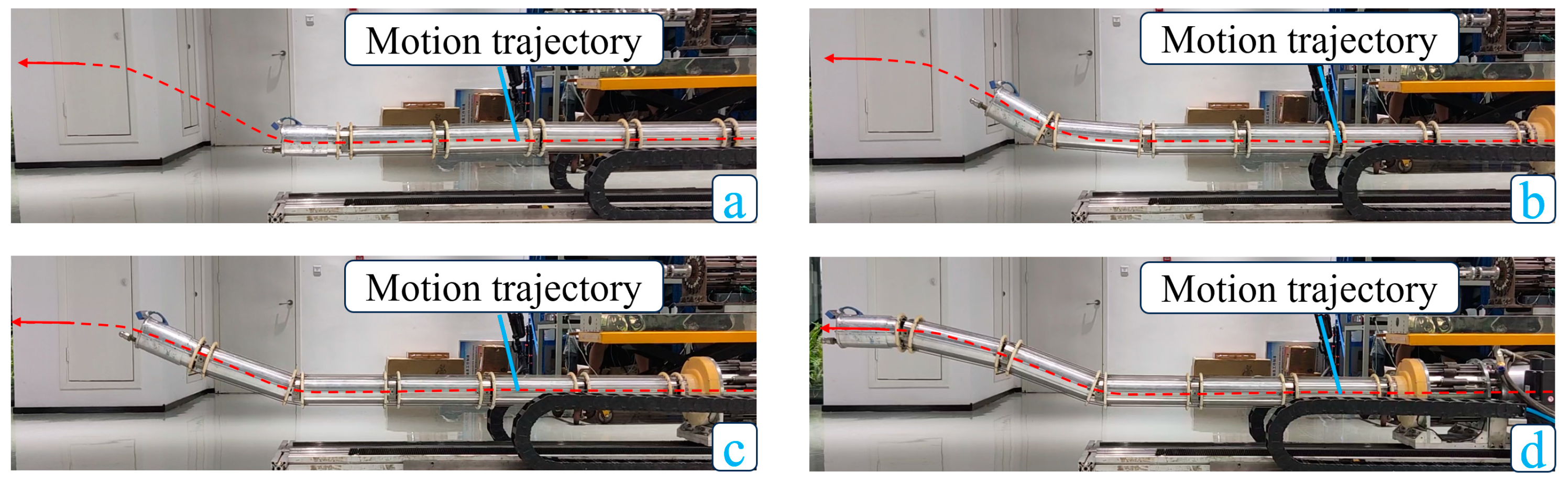
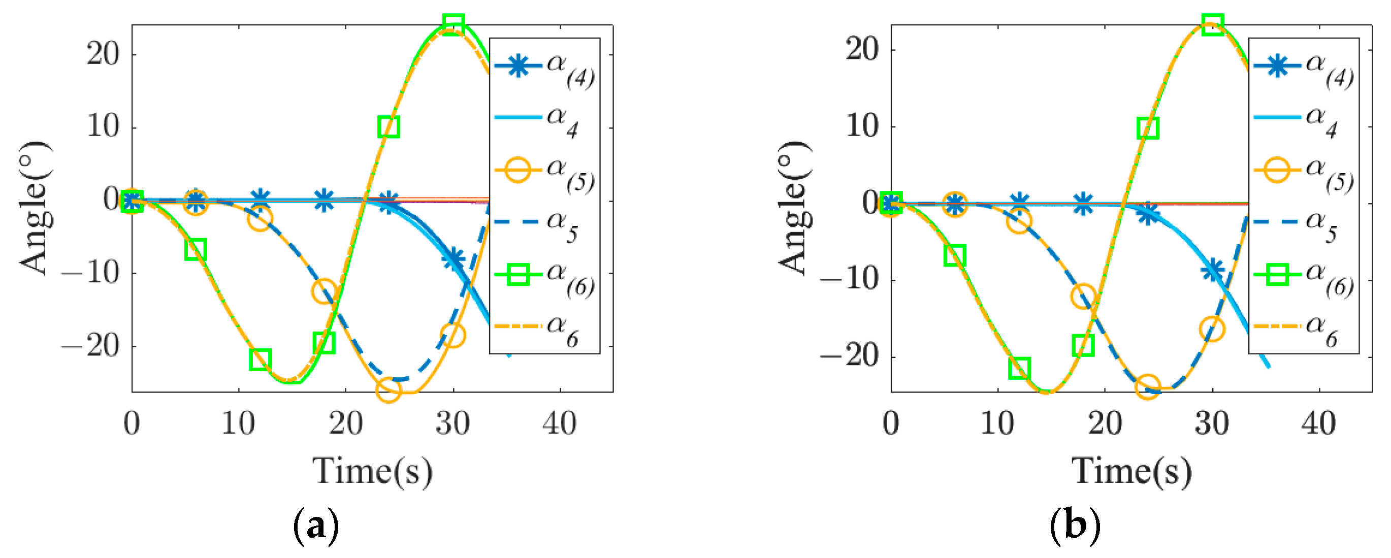
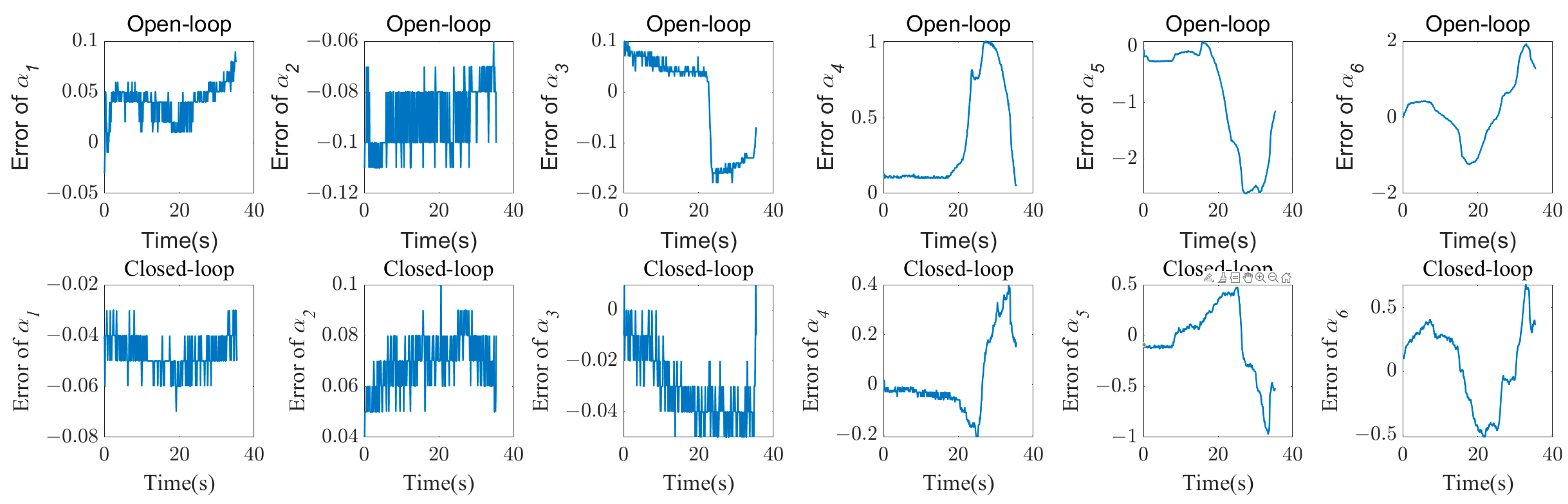
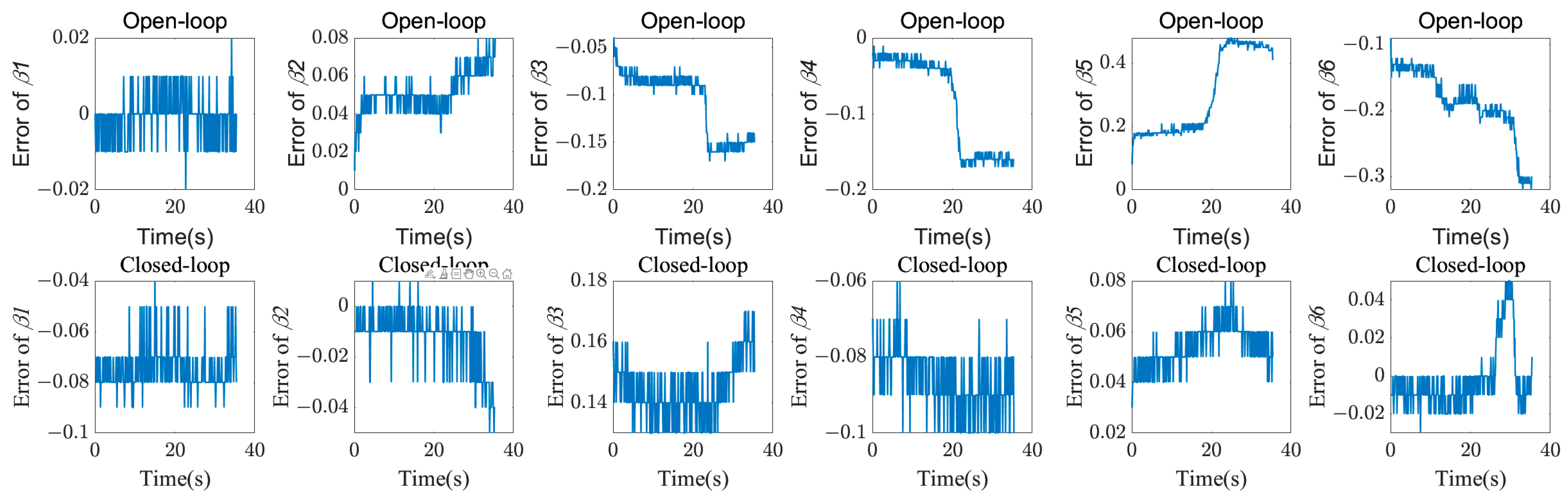
6.3. Continuous Motion Test

Continuous motion test refers to comparing the dynamic performance of each control strategy when the CSR moves along the planned path. Because of the instability of the single-loop, the paper has not conducted a continuous motion test of this motion mode. Figure 11 shows the photos of CSR during the motion. During the test, CSR performed the tip-following motion, i.e., the centers of all joints would follow the motion trajectory of the CSR’s end. The photos have been sorted alphabetically according to the motion sequence. Figure 12a shows the variation in the joint angles when the CSR executes the open-loop motion mode. Figure 12b shows the variation in the joint angles when the CSR executes the dual-loop motion mode. In the figures, ${\alpha }_4,{\alpha }_5,{\alpha }_6$ correspond to the desired values, and ${\alpha }_{\left(4\right)},{\alpha }_{\left(5\right)},{\alpha }_{\left(6\right)}$ correspond to the feedback joint angles.

If we take the joint angle errors as the research object, then the relationships between the errors and time can be shown in Figure 13. The figures show the errors are relatively smaller with the closed-loop control, especially when the joint angles are large. Furthermore, when the proximal joints keep still, their joint angle errors of the open-loop control are tiny. That is because the cables driving these proximal joints keep still, which can effectively promise the stillness of these proximal joints.

Furthermore, the CSR’s quantitative performance could be analyzed with the integral square error (ISE) criteria. The corresponding ISE values are,

$$\mathit{I}\mathit{S}{\mathit{E}}_{\mathit{o}\mathit{p}\mathit{e}\mathit{n}}=\left[\begin{array}{ccc}IS{E}_{\alpha 1}& & IS{E}_{\beta 1}\\ ⋮& & ⋮\\ IS{E}_{\alpha 6}& & IS{E}_{\beta 6}\end{array}\right]={\left[\begin{array}{cc}\begin{array}{ccc}0.069& 0.294& 0.328\end{array}& \begin{array}{ccc}8.600& 63.949& 24.320\end{array}\\ \begin{array}{ccc}0.001& 0.096& 0.452\end{array}& \begin{array}{ccc}0.389& 3.778 & 1.341\end{array} \end{array}\right]}^{\mathit{T}}$$

(35)

$$\mathit{I}\mathit{S}{\mathit{E}}_{\mathit{c}\mathit{l}\mathit{o}\mathit{s}\mathit{e}\mathit{d}}={\left[\begin{array}{cc}\begin{array}{ccc}0.082& 0.174& 0.039\end{array}& \begin{array}{ccc}0.740& 4.202& 3.769\end{array}\\ \begin{array}{ccc}0.198& 0.010& 0.742\end{array}& \begin{array}{ccc}0.265& 0.107& 0.010\end{array}\end{array}\right]}^{\mathit{T}}$$

(36)

$IS{E}_{\alpha 1}(i=1,2,\dots 6)$: ISE value of ${\alpha }_1$.

$IS{E}_{\beta 1}(i=1,2,\dots 6)$: ISE value of ${\beta }_1$.

$\mathit{I}\mathit{S}{\mathit{E}}_{\mathit{o}\mathit{p}\mathit{e}\mathit{n}}$: ISE value of all the joint angles corresponding to open-loop.

$\mathit{I}\mathit{S}{\mathit{E}}_{\mathit{c}\mathit{l}\mathit{o}\mathit{s}\mathit{e}\mathit{d}}$: ISE value of all the joint angles corresponding to closed-loop.

The continuous motion test results show that CSR is unable to adjust its posture in the open-loop motion mode, resulting in poor motion accuracy. In particular, when the joint angle is relatively large, the errors will expand more severely. On the contrary, the dual-loop motion mode has a good tracking performance on the expected trajectory. That indicates its dynamic and steady-state accuracy are both relatively high.

6.4. Discussion

According to Section 5.1, there are multiple types of errors during CSR’s motion. All of these will affect CSR’s accuracy. Thus, the closed-loop control can significantly improve its motion effect. The three types of experiments show the dual-loop mode always has the best steady-state and dynamic performance. In particular, during the continuous motion test, the CSR in dual-loop motion mode not only has higher accuracy but also smoother motion. That successfully verifies the feasibility and superiority of the dual-loop control strategy.

According to Section 5.2, the instability may occur during the continuous execution of the single-loop mode, i.e., the single-loop mode is without a reliable steady-state. The tests of Section 6.1 and Section 6.2 show that the more rotating joints and the greater the rotation angles, the more pronounced the instability. In contrast, the dual-loop control strategy notably improves the accuracy of each joint and maintains the motion accuracy well. That verifies the importance of the force-loop.

In essence, the dual-loop control strategy not only solves the problem of low accuracy in the open-loop mode, but also solves the defect of low stability in the single-loop mode. After verification, the dual-loop mode can greatly improve the motion performance of CSR and meet the requirements of most engineering applications.

7. Conclusions

This article designs a type of cable-driven snake-like robot. The robot not only has joint angle sensors to detect the robot posture status, but also has force transducers to collect the driving force data of the cables. Moreover, these two sensors are installed on the CSR in a very compact way via the ingenious structural design. Afterwards, through studying the kinematic model based on the link eigen vectors and the corresponding inverse dynamics, the kinematic and dynamic variables needed for dual-loop control could be calculated. As a result of studying the sources of the errors during CSR’s motion and the practicability of closed-loop control, a reliable, stable, and high-precision dual-loop control strategy is proposed. Finally, the experiments have fully proved the effectiveness of the dual-loop control strategy.

In the future, we will study a more intelligent control strategy that can automatically adjust the PID parameters according to the environment load. Moreover, the sources of error will be subjected to more elaborate analysis. Thus, the more adaptable and accurate control strategy of CSR can be realized.

References

1. Chirikjian, G.S.; Burdick, J.W. An obstacle avoidance algorithm for hyper-redundant manipulators. In Proceedings of the IEEE International Conference on Robotics and Automation, Cincinnati, OH, USA, 13–18 May 1990; pp. 625–631. [Google Scholar]
2. Liu, T.; Xu, W.; Yang, T.; Li, Y. A hybrid active and passive cable-driven segmented redundant manipulator: Design, kinematics, and planning. IEEE/ASME Trans. Mechatron. 2021, 26, 930–942. [Google Scholar] [CrossRef]
3. Chikhaoui, M.T.; Lilge, S.; Kleinschmidt, S.; Burgner-Kahrs, J. Comparison of modeling approaches for a tendon actuated continuum robot with three extensible segments. IEEE Robot. Automat. Lett. 2019, 4, 989–996. [Google Scholar]
4. Liao, B.; Zang, H.; Chen, M.; Wang, Y.; Lang, X.; Zhu, N.; Yang, Z.; Yi, Y. Soft rod-climbing robot inspired by winding locomotion of snake. Soft Robot. 2020, 7, 500–511. [Google Scholar] [CrossRef] [PubMed]
5. Hannan, M.W.; Walker, I.D. Kinematics and the implementation of an elephant’s trunk manipulator and other continuum style robots. J. Robot. Syst. 2003, 20, 45–63. [Google Scholar] [CrossRef]
6. Kim, J.; Kwon, S.; Moon, Y.; Kim, K. Cable-movable rolling joint to expand workspace under high external load in a hyper-redundant manipulator. IEEE/ASME Trans. Mechatron. 2022, 27, 501–512. [Google Scholar] [CrossRef]
7. Burgner-Kahrs, J.; Rucker, D.C.; Choset, H. Continuum robots for medical applications: A survey. IEEE Trans. Robot. 2015, 31, 1261–1280. [Google Scholar] [CrossRef]
8. Hong, W.; Xie, L.; Liu, J.; Sun, Y.; Li, K.; Wang, H. Development of a novel continuum robotic system for maxillary sinus surgery. IEEE/ASME Trans. Mechatron. 2018, 23, 1226–1237. [Google Scholar] [CrossRef]
9. Xu, K.; Zhao, J.; Fu, M. Development of the SJTU unfoldable robotic system (SURS) for single port laparoscopy. IEEE/ASME Trans. Mechatron. 2015, 20, 2133–2145. [Google Scholar] [CrossRef]
10. Buckingham, R.; Graham, A. Nuclear snake-arm robots. Ind. Rob. 2012, 39, 6–11. [Google Scholar] [CrossRef]
11. Tonapi, M.M.; Godage, I.S.; Walker, I.D. Next generation rope-like robot for in-space inspection. In Proceedings of the 2014 IEEE Aerospace Conference, Big Sky, MT, USA, 1–8 March 2014; pp. 1–13. [Google Scholar]
12. Chavan, P.; Murugan, M.; Unnikkannan, E.V.; Singh, A.; Phadatare, P. Modular snake robot with mapping and navigation: Urban search and rescue robot. In Proceedings of the 2015 International Conference on Computing Communication Control and Automation, Pune, India, 26–27 February 2015. [Google Scholar]
13. Tsukagoshi, H.; Kitagawa, A.; Segawa, M. Active hose: An artificial elephant’s nose with maneuverability for rescue operation. In Proceedings of the IEEE International Conference on Robotics and Automation, Seoul, Republic of Korea, 21–26 May 2001; pp. 2454–2459. [Google Scholar]
14. Naccarato, F.; Hughes, P.C. Inverse kinematics of variable-geometry truss manipulators. J. Robot. Syst. 1991, 8, 249–266. [Google Scholar] [CrossRef]
15. Chirikjian, G.S.; Burdick, J.W. A geometric approach to hyper-redundant manipulator obstacle avoidance. J. Mech. Des. 1992, 114, 580–585. [Google Scholar] [CrossRef]
16. Chirikjian, G.S.; Burdick, J.W. A modal approach to hyper-redundant manipulator kinematics. IEEE Trans. Robot. Autom. 1994, 10, 343–354. [Google Scholar] [CrossRef]
17. Xie, H.; Wang, C.; Li, S.; Hu, L.; Yang, H. A geometric approach for follow-the-leader motion of serpentine manipulator. Int. J. Adv. Robot. Syst. 2019, 16, 172988141987463. [Google Scholar] [CrossRef]
18. Sreenivasan, S.; Goel, P.; Ghosal, A. A real-time algorithm for simulation of flexible objects and hyper-redundant manipulators. Mech. Mach. Theory 2010, 45, 454–466. [Google Scholar] [CrossRef]
19. Aristidou, A.; Lasenby, J. FABRIK: A fast, iterative solver for the Inverse Kinematics problem. J. Robot. Syst. 2011, 73, 243–260. [Google Scholar] [CrossRef]
20. Rodriguez, G. Kalman filtering, smoothing, and recursive robot arm forward and inverse dynamics. IEEE J. Rob. Autom. 1987, 3, 624–639. [Google Scholar] [CrossRef]
21. Falkenhahn, V.; Mahl, T.; Hildebrandt, A.; Neumann, R.; Sawodny, O. Dynamic modeling of bellows-actuated continuum robots using the Euler–Lagrange formalism. IEEE Trans. Robot. 2015, 31, 1483–1496. [Google Scholar] [CrossRef]
22. Campisano, F.; Caló, S.; Remirez, A.; Chandler, J.; Obstein, K.; Webster, R.; Valdastri, P. Closed-loop control of soft continuum manipulators under tip follower actuation. Int. J. Robot. Res. 2021, 40, 923–938. [Google Scholar] [CrossRef]
23. Xu, W.; Liu, T.; Li, Y. Kinematics, dynamics, and control of a cable-driven hyper-redundant manipulator. IEEE/ASME Trans. Mechatron. 2018, 23, 1693–1704. [Google Scholar] [CrossRef]
24. Li, W.; Huang, X.; Yan, L.; Cheng, H.; Liang, B.; Xu, W. Force sensing and compliance control for a cable-driven redundant manipulator. IEEE/ASME Trans. Mechatron. 2023, 1–12. [Google Scholar] [CrossRef]
25. Tran, L.D.; Zhang, Z.; Yeo, S.H.; Sun, Y.C.; Yang, G.L. Control of a cable-driven 2-DOF joint module with a flexible backbone. In Proceedings of the IEEE Conference on Sustainable Utilization and Development in Engineering and Technology (STUDENT), Semenyih, Malaysia, 20–21 October 2011; pp. 150–155. [Google Scholar]
26. Sun, Z.; Wang, Z.; Phee, S.J. Modeling and motion compensation of a bidirectional tendon-sheath actuated system for robotic endoscopic surgery. Comput. Methods Programs Biomed. 2015, 119, 77–87. [Google Scholar] [CrossRef] [PubMed]
27. Tang, J.; Zhang, Y.; Huang, F.; Li, J.; Chen, Z.; Song, W.; Zhu, S.; Gu, J. Design and kinematic control of the cable-driven hyper-redundant manipulator for potential underwater applications. Appl. Sci. 2019, 9, 1142. [Google Scholar] [CrossRef]
28. Roesthuis, R.J.; Misra, S. Steering of multisegment continuum manipulators using rigid-link modeling and FBG-based shape sensing. IEEE Trans. Robot. 2016, 32, 372–382. [Google Scholar] [CrossRef]
29. Park, Y.-L.; Ryu, S.C.; Black, R.J.; Chau, K.K.; Moslehi, B.; Cutkosky, M.R. Exoskeletal force-sensing end-effectors with embedded optical fiber-Bragg-grating sensors. IEEE Trans. Robot. 2009, 25, 1319–1331. [Google Scholar] [CrossRef]
30. Bajo, A.; Simaan, N. Hybrid motion/force control of multi-backbone continuum robots. Int. J. Robot. Res. 2016, 35, 422–434. [Google Scholar] [CrossRef]
31. Xu, X.; Xie, H.; Wang, C.; Yang, H. Kinematic and dynamic models of hyper -redundant manipulator based on link eigenvectors. IEEE/ASME Trans. Mechatron. 2023, 1–13. [Google Scholar] [CrossRef]
Figure 1. Overview of CSR.
Robotics 12 00126 g001
Figure 2. Base box: (a) Structure of base box; (b) setup of force transducer.
Robotics 12 00126 g002
Figure 3. Robot arm: (a) Structure of robot arm; (b) setup of angle sensor.
Robotics 12 00126 g003
Figure 4. Analysis of cable force and interaction force.
Robotics 12 00126 g004
Figure 5. First type of errors.
Robotics 12 00126 g005
Figure 6. Second type of errors.
Robotics 12 00126 g006
Figure 7. Pose-loop control strategy.
Robotics 12 00126 g007
Figure 8. Closed-loop process of the driving of one cable in J o i n t i
Robotics 12 00126 g008
Figure 9. Block diagram of the dual-loop control strategy.
Robotics 12 00126 g009
Figure 10. Multiple joints motions: (a) Motion of multiple pitch joints; (b) motion of multiple yaw joints; (c) composite motion of multiple pitch and yaw joints.
Robotics 12 00126 g010
Figure 11. Dynamic motion: (a) First step; (b) second step; (c) third step; (d) fourth step.
Robotics 12 00126 g011
Figure 12. Variation of joint angles: (a) Open-loop; (b) dual-loop.
Robotics 12 00126 g012
Figure 13. Relationships between the errors and time.
Robotics 12 00126 g013aRobotics 12 00126 g013b