Online Motion Planning for Safe Human–Robot Cooperation Using B-Splines and Hidden Markov Models

Abstract

When humans and robots work together, ensuring safe cooperation must be a priority. This research aims to develop a novel real-time planning algorithm that can handle unpredictable human movements by both slowing down task execution and modifying the robot’s path based on the proximity of the human operator. To achieve this, an efficient method for updating the robot’s motion is developed using a two-fold control approach that combines B-splines and hidden Markov models. This allows the algorithm to adapt to a changing environment and avoid collisions. The proposed framework is thus validated using the Franka Emika Panda robot in a simple start–goal task. Our algorithm successfully avoids collision with the moving hand of an operator monitored by a fixed camera.

1. Introduction

In modern industries, the demand for collaborative robots is constantly increasing because of their versatility and precision in a wide variety of applications. In a collaborative cell, humans and robots work together, sharing the same workspace. Therefore, the robot must adapt to external events while complying with safety regulations [1]. Safe human–robot cooperation can be achieved if the control system can gather information about the state of the robot as well as the state of the worker inside the collaborative workspace. Obstacle avoidance algorithms are employed whenever the presence of a target, such as an object or an operator, should be accounted for in the proper and safe operation of the robot. The latter must be able to adapt its behavior in real time with respect to dynamically changing environments [1,2].

In general obstacle avoidance applications [3], the robot uses the position of a target object to modify its path and avoid colliding with it. Although safety distance margins can be imposed on the target object, unexpected movements can cause the robot to collide if the algorithm is not reactive enough to prevent the impact [4]. On the other hand, the planning algorithm should consider restoring the original path once the operator is outside the workspace so the robot can run its task in nominal conditions [5].

In this work, the moving obstacle is represented by the hand of a human operator who shares the same workspace as a cobot and whose position is monitored by a fixed camera. The robot must repeat a preplanned task, but according to the proposed framework, when the risk of a collision occurs, it can either modify the geometry of the path or reduce its velocity according to the requirements of the specific application. Then, when the obstacle is no longer within the robot’s reach, the programmed motion is restored.

The literature is full of methods that guarantee obstacle avoidance and the safe coexistence of humans and robots. To highlight the contribution of our proposal, the main state-of-the-art techniques are reviewed and briefly discussed in the following.

1.1. Related Work

Collision avoidance methods for robotic systems operating in dynamic environments with obstacles moving at high velocity typically rely on a combination of real-time trajectory planning and reactive control. These methods may vary in their level of integration, ranging from pure re-planning to the use of repulsive forces that act directly on the robot.

Collision avoidance motion planning problems can be, first of all, treated as an optimal control problem [6]. These approaches are widely used because they allow for the minimization of cost functions subject to disparate constraints, such as danger fields, temporal aspects, or even metrics for evaluating safety in collaborative manufacturing [4,7]. Optimization methods can be applied to both motion planning and control problems. A noteworthy optimization-based algorithm is CHOMP [8], i.e., Covariant Hamiltonian Optimization for Motion Planning, which guarantees collision-free and locally optimal trajectory generation by means of a covariant gradient update rule. Another example is presented in [9], where a parallel optimization scheme is successfully used to manipulate a cable-towed load with multiple collaborative quadrupeds.

Probabilistic inference methods [10,11,12] optimize trajectories subject to task constraints, goals, and motion priors, replacing classical cost functions with joint distributions formulated as conditional dependencies. In [13], the author introduces a Learning by Demonstration (LbD) framework that exploits Gaussian Mixture Models (GMM) to encode multiple tasks and retrieve the associated skill by means of regression techniques.

A different class of methods for motion planning and collision avoidance is composed of so-called sample-based planning algorithms [14]; according to these approaches, the environment is randomly sampled using techniques such as probabilistic road maps or exploring random trees. An example is given in [15], where sampled via-points are transformed into a set of candidate collision-free trajectories subject to predefined kinodynamic limits. In [16], if a moving obstacle collides with the manipulator, the motion is locally re-planned by using a Bi-RRT-based algorithm connecting the current robot position with a target on the unperturbed trajectory.

While the above-mentioned algorithms mainly work at the planning levels, an approach for reactive collision avoidance that acts directly on the robot control relies on potential field methods, originally introduced in [17]. Virtual repulsive and attractive fields are utilized to move the robot towards a target while avoiding obstacles. Specifically, repulsive fields are associated with obstacles, while attractive fields are associated with the target. The original concept has been further refined and applied to properly modify the shape of motion trajectories, which are seen as elastic bands subject to virtual forces [18], and is now a standard technique for real-time trajectory planning [3,19].

If all the techniques cited above modify the geometry of the robot motion, state-of-the-art methods in the industrial practice for guaranteeing safety in human–robot applications are based on a completely different philosophy [20]. They basically consist of stopping or slowing down robot motion in the presence of humans. For instance, according to ISO/TS 15066, the velocity and acceleration of the robot must be set to safe values based on the minimum distance from the operator [21]. This approach is commonly used in collaborative applications, where the position of human workers is continuously monitored with different types of cameras and the timing along the curve is properly scaled. See, for example, Refs. [7,22,23], among many other publications on this topic. Note that, in the case of dynamic obstacles, this technique based on the velocity modulation of the robot can also be a way to avoid obstacles that are currently on the desired geometric path but could move in the following instants.

1.2. Methodology and Contributions

In this work, we propose a novel framework for collision avoidance that merges the modification of the geometric path of the robot with a speed adaptation mechanism. The basic idea, derived from observations reported in [24], is to split the task representation into two fundamental categories: the trajectory and the symbolic level. The former comprises continuous signals that change over time, such as the position or orientation of the end effector (EE); the latter uses sequential or hierarchical information to establish a discrete set of movements with predefined rules. The goal of this work is to provide evidence, through an obstacle avoidance application, that task performance can benefit from the merging of these two domains.

The two basic tools used to implement this framework are B-splines, which encode spatial data and modify the path in Cartesian space [25], and hidden Markov models (HMMs), which encode temporal and sequential information by scaling down task velocity [26].

The main goals and contributions of this research work are to:

• Design an online controller that can fit generic tasks and smoothly avoid collisions with dynamic obstacles.
• Include the possibility to restore the original task whenever the robot is not prone to any collision.
• Exploit a probabilistic framework to gather information about the obstacle and modify the robot’s velocity accordingly.
• Combine trajectory and symbolic domains in a unified framework.

The paper is structured as follows: Section 2 details the theoretical background of the proposed solution. Section 3 describes the online control algorithm conceived in this work. Section 4 describes the experimental setup and validates the results of our framework. Finally, Section 5 concludes this work by discussing the results and possible future steps.

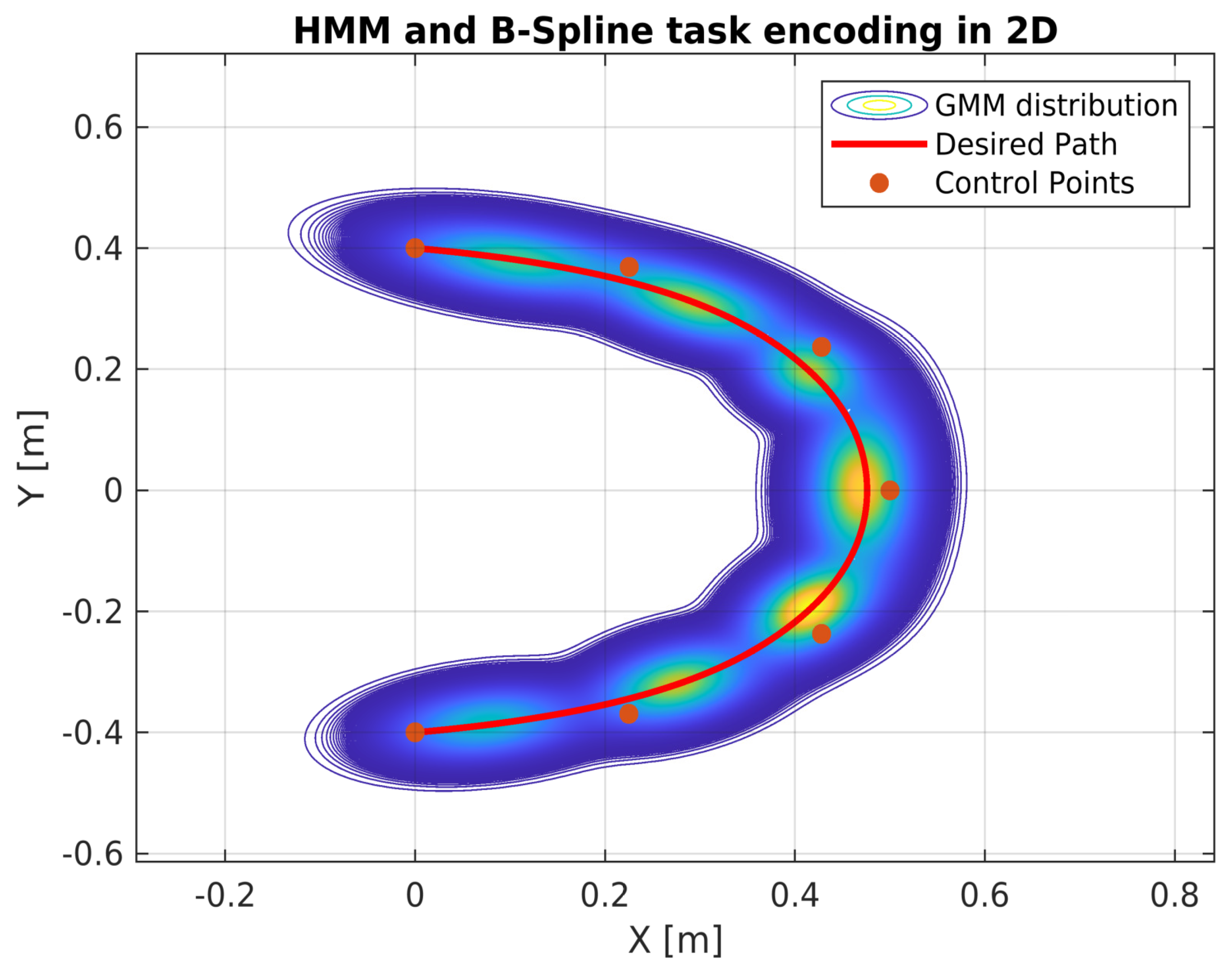
2. Task Encoding

The simplest way to define a robotic task is by specifying the trajectory, which is a mapping between time and space, that the end effector or joints must track. However, a task can also be interpreted as a sequence of action units or elements that follow loops or rules, as is the case with a symbolic representation as seen in [27,28].

This work attempts to bridge and combine these two domains for an obstacle avoidance application. This is achieved through a control system that modifies the nominal robot path defined by B-spline functions [25] while also varying the phase of the task, and thus its velocity, using an HMM [26]. The following paragraphs provide a brief review of the theoretical background of these techniques.

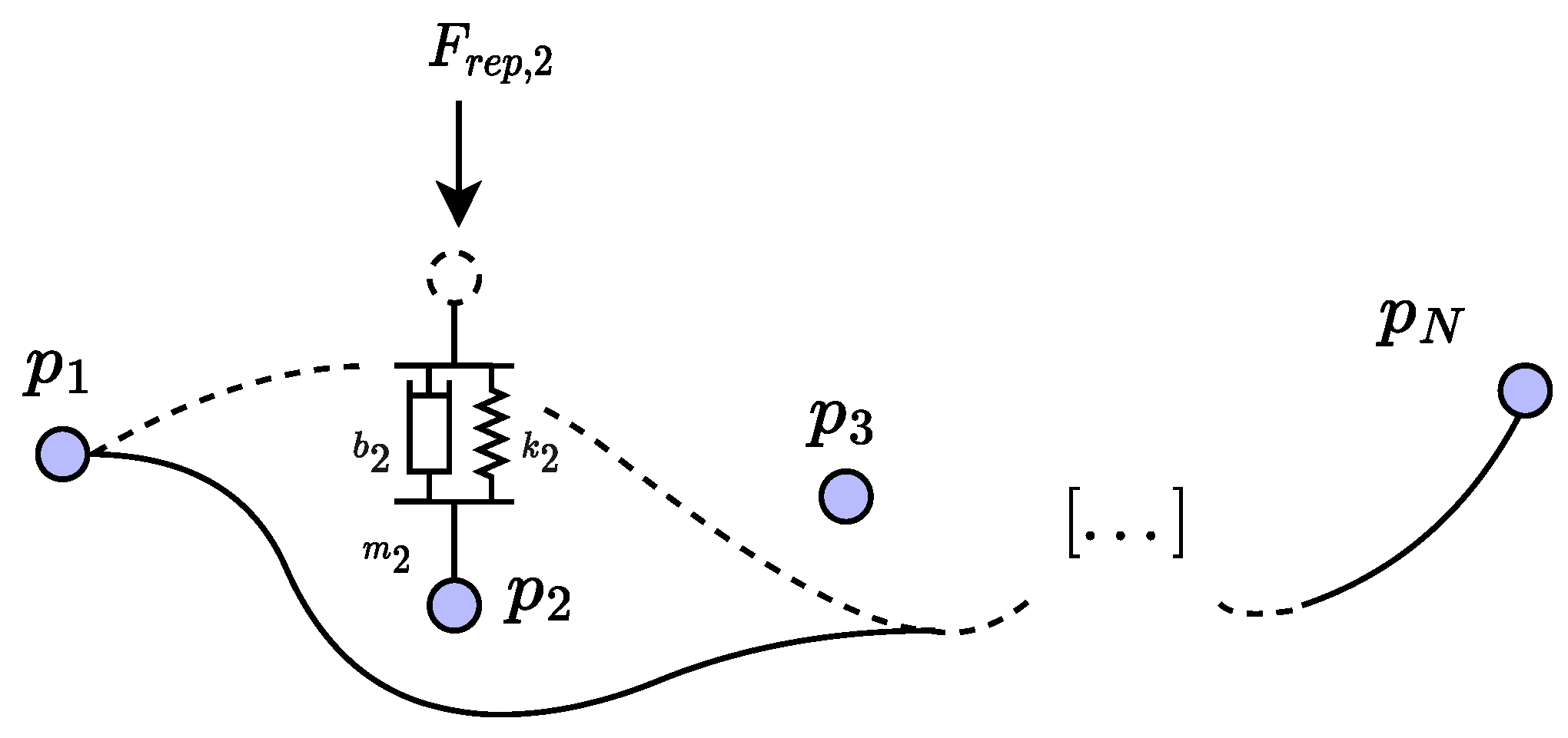
2.1. Spatial Encoding Based on B-Splines

Spline functions are extensively used for generating smooth and optimal time trajectories in robotic applications [15,29,30]. B-splines are a particular representation of generic spline curves based on a linear combination of N basis functions [29], i.e.,

$$\mathit{p}\left(s\right)=\sum _{i=1}^N{\mathit{p}}_i{\beta }_i^d\left(s\right),s_{min}\le s\le s_{max}$$

(1)

where ${\beta }_i^d\left(s\right)$ are basis functions of degree d, which only depends on the phase variable s (that in many applications coincides with time t), while ${\mathit{p}}_i$ are called control points and determine the geometric shape of the curve. As shown in Figure 1, a B-spline is basically a smooth approximation of the control polygon defined by the control points. Usually, they are defined by imposing some interpolation condition $\mathit{p}\left(s_i\right)={\mathit{p}}_i,i=1,\dots ,N$, depending on the desired task.

A noteworthy property of the basis functions ${\beta }_i^d\left(s\right)$ is that their value is zero everywhere except in the interval defined by knots $[s_i,s_{i+d+1}]$. As a consequence, a change in the i-th control point ${\mathit{p}}_i$ only influences the B-spline in this interval, allowing for local modifications in the trajectory described. Another useful property of B-splines is time-scaling, i.e., the possibility of changing the velocity along the curve by simply applying the transformation $\widehat{s}=\alpha s$ to the knot vector s, where $\alpha$ is a constant. For more details, see [25].

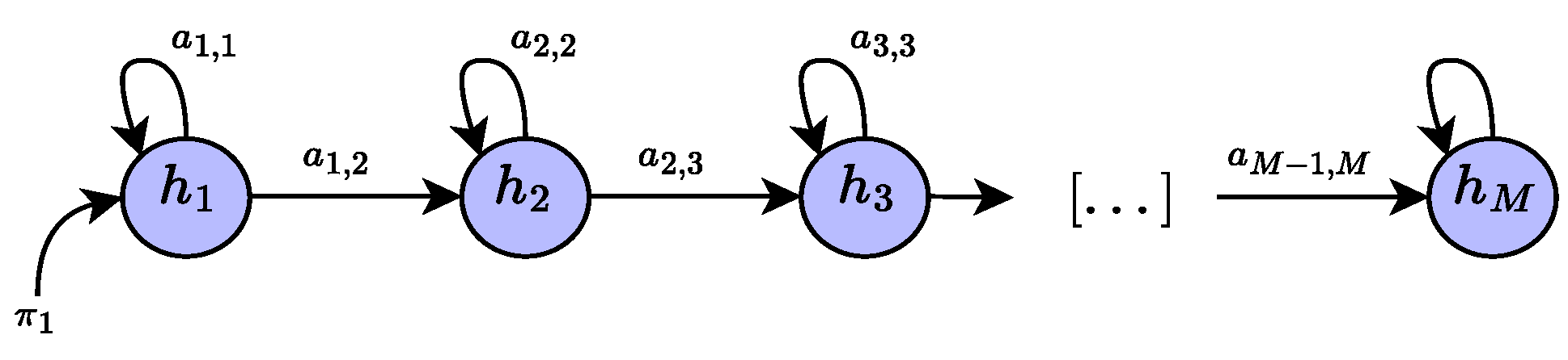
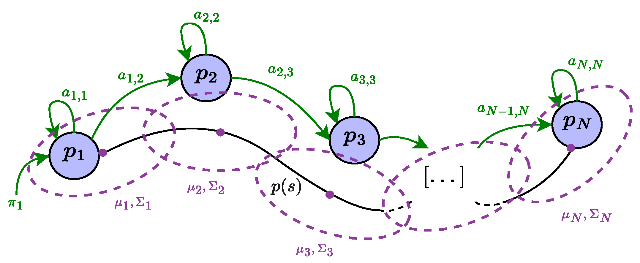
2.2. Temporal and Sequential Encoding Based on Hidden Markov Models

Hidden Markov models (HMMs) are based on a Markov chain, which describes the probabilities of sequences of random variables, called states, that take values from a defined set [31]. In many applications, such as gesture and speech recognition [26,28], HMMs are used to model human behavior, with the aim of identifying gestures or predicting the most likely pattern of subsequent control states. Specifically, given a set of hidden states $H=h_1,h_2,\dots ,h_M$ and a sequence of T observations $O=o_1,o_2,\dots ,o_T$, the purpose of HMMs is to analyze sequences of events in terms of a reduced set of parameters $\mathit{\lambda }=[\mathbf{\Pi },\mathbf{A},\mathbf{B}]$, where:

• $\mathbf{\Pi }$ is called the prior distribution, which tells us about the probability of starting a sequence in state $h_i$;
• $\mathbf{A}$ is the transition probability matrix, where each element $a_{i,j}$ encodes the probability of moving from state i to state j;
• $\mathbf{B}$ are the observation likelihoods, also called emission probabilities, where each element $b_i\left(o_t\right)$ expresses the probability of an observation $o_t$ being generated from state i.

Note that, according to the usual definition of HMMs, $\mathit{\lambda }$ describes a model in terms of discrete observation likelihoods [32]. However, since the proposed framework deals with a continuous observation space, i.e., trajectories in Cartesian space, the HMM can be represented as

$$\mathit{\lambda }=[\mathbf{\Pi },\mathit{A},{\mathit{\mu }}_i,{\mathbf{\Sigma }}_i]i=1,\dots ,M$$

(2)

where M is the number of components characterized by mean and covariance values $({\mathit{\mu }}_i,{\mathbf{\Sigma }}_i)$ of the multivariate Gaussian Mixture Model (GMM). Thus, the $\mathit{\lambda }$ parameters can be learned to encode the desired robot task, such that the regression of the model resembles the desired end effector path [33].

The proposed methodology can be explained as follows: using control points ${\mathit{p}}_i$ as hidden states $h_i$, a forward-chained left–right HMM is adopted (see Figure 2) to account for the evolution of the trajectory [34]. With this model, in nominal conditions (i.e., no obstacles in the workspace), ${\pi }_1=1$ and transition probabilities $a_{i,i+1}\approx 1$, meaning that the robot evolves from one control point to the other with a probability close to one. In particular, let us analyze the transition matrix A for the HMM in Figure 2:

$$\mathit{A}=\left[\begin{array}{cccccc}{a}_{11}& a_{12}& 0& \cdots & 0& 0\\ 0& a_{22}& a_{23}& \cdots & 0& 0\\ ⋮& ⋮& ⋮& \ddots & ⋮& ⋮\\ 0& 0& 0& \cdots & a_{M-1M-1}& a_{M-1M}\\ 0& 0& 0& \cdots & 0& a_{MM}\end{array}\right]$$

(3)

Here, the elements of each row of A sum up to 1. Parameter $a_{i,i}$ is the probability of staying in state $h_i$, while $a_{i,i+1}$ is the probability of moving from state $h_i$ to state $h_{i+1}$. Thus, the transition probabilities $a_{i,i+1}$ can be used to slow down or eventually stop the robot every time their values warn the system about a potential collision, as is explained in the next section.

3. Proposed Method

We consider a typical industrial scenario in which a robot is required to perform a specific task within a monitored workspace, using a fixed camera. When an obstacle enters the workspace, such as the hand of a human operator, its actual position is tracked, filtered through a Kalman filter, and sent to the controller that implements the proposed framework in order to prevent possible collisions. The functional blocks of the entire algorithm are displayed in the scheme shown in Figure 3, while the working principles are detailed below.

3.1. Spatial Modulation with Dynamical Control Points

Given the presence of moving obstacles, we assume that the task is modified only if they interfere with the nominal trajectory. However, if the obstacles move far from the robot, the task should be restored to its original trajectory. To achieve this, we use B-spline functions to induce a reversible deformation on the original trajectory. Specifically, a dynamical system is associated with each control point ${\mathit{p}}_i$ [5]:

$${\mathit{M}}_i,{\ddot{\tilde{\mathit{p}}}}_i+{\mathit{B}}_i,{\dot{\tilde{\mathit{p}}}}_i+{\mathit{K}}_i,\tilde{\mathit{p}}i={\mathit{F}}_{rep,i}$$

(4)

where, ${\tilde{\mathit{p}}}_i={\mathit{p}}^{\left(i\right)}-{\mathit{p}}_i$ represents the displacement of the actual position ${\mathit{p}}^{\left(i\right)}$ of the i-th control point with respect to its original location ${\mathit{p}}_i$. The matrices ${\mathit{M}}_i=\mathrm{diag}\left\{m_i\right\}$, ${\mathit{B}}_i=\mathrm{diag}\left\{b_i\right\}$, and ${\mathit{K}}_i=\mathrm{diag}\left\{k_i\right\}$ are 3-by-3 diagonal matrices, where $m_i$, $b_i$, and $k_i$ are positive constants such that the system in (4) is critically damped. This can be performed by choosing, for example, $m_i={\widehat{m}}_i$ and $k_i={\widehat{k}}_i$, then computing $b_i$ as ${\widehat{b}}_i=2\sqrt{{\widehat{m}}_i·{\widehat{k}}_i}$. Finally, ${\mathit{F}}_{rep,i}$ is a virtual repulsive force applied in the direction from the obstacle to the i-th control point.

This idea is explained in Figure 4. The module of the repulsive force ${\mathit{F}}_{rep,i}$ acting on the i-th control point does not depend on its Cartesian distance from the obstacle but varies in intensity according to the Mahalanobis distance:

$$D_M(\mathit{x},\mathit{\mu },\mathbf{\Sigma })=\sqrt{{(\mathit{x}-\mathit{\mu })}^T{\mathbf{\Sigma }}^{-1}(\mathit{x}-\mathit{\mu })}$$

(5)

that accounts for the occupation probability of the obstacle ${\widehat{\mathit{p}}}_{obs}\sim \mathcal{N}({\mathit{\mu }}_{obs},{\mathbf{\Sigma }}_{obs})$, caused by uncertainties in the estimation of its location [6,35]. The module of the force can therefore be computed as follows [6]

$$|F_{rep,i}|=\frac{{\chi }_i}{D_M({\mathit{p}}^{\left(i\right)};{\mathit{\mu }}_{obs},{\mathbf{\Sigma }}_{obs})}$$

(6)

where ${\chi }_i$ is a free parameter that enables the repulsive force field intensity to be varied. Finally, the path is encoded with a third-order B-spline such that its derivatives are continuous until the acceleration, with limited jerk. This is of fundamental importance and should be designed carefully as, from a practical point of view, the internal inverse kinematics algorithm could lead to a joint acceleration discontinuity error if the trajectory overcomes the robot’s limitations [29].

3.2. Temporal Modulation with Varying Transition Probabilities in HMM

In our framework, the path of the task is encoded by $\mathit{p}\left(s\right)$ in (1), while velocity is varied through the HMM’s parameters $\mathit{\lambda }$, accounting for the temporal modulation.

The connection between B-splines and the HMM domains is established through the continuous observation likelihoods $\mathcal{N}({\mathit{\mu }}_i,{\mathbf{\Sigma }}_i)=b_i\left(o_t\right)$, $i=1,\dots ,M$, as shown in (2). In particular, $({\mathit{\mu }}_i,{\mathbf{\Sigma }}_i)$ are the components of a GMM that encodes the likelihood of a point $\mathit{r}\in {\mathbb{R}}^3$ being described by the HMM’s model $\mathit{\lambda }$:

$$\mathbf{B}\sim P\left(\mathit{r}\right)=\sum _{i=1}^M{\mathcal{W}}_i\left(\mathit{r}\right)\mathcal{N}(\mathit{r};{\mathit{\mu }}_i,{\mathbf{\Sigma }}_i)$$

(7)

where the weighting factor $\mathcal{W}i$ with ${\sum }_{i=1}^M{\mathcal{W}}_i=1$ is called the mixing coefficient and represents the influence of the i-th component [13]. Gaussian distributions are encoded such that their regression corresponds to the nominal trajectory $\mathit{p}\left(s\right)$ [36]. Furthermore, in (7), $\mathbf{B}$ accounts for the variability introduced by the movement of control points, thus giving a stochastic topological representation of the task. Figure 5 illustrates a graphical representation of this approach. It is worth noting that the number of states M of the HMM is generally different from the number of control points N that define the B-spline. For instance, it is possible to encode with the same state a segment of the trajectory curve, corresponding to a subtask, composed of several control points. However, for the sake of simplicity, it is convenient to assume $M=N$.

As explained in Section 2, the evolution of the B-spline trajectory can be modified by applying the transformation $\widehat{s}=\alpha s$ to the knots vector of $\mathit{p}\left(s\right)$. In this way, the desired velocity $\dot{s}$ is multiplied by a factor $\alpha \in [0,1]$ and reduced accordingly. To implement a mechanism that is able to slow down the robot and eventually stop it in the case of a collision risk, the transition probabilities of the HMM are directly mapped into proper values of $\alpha$, as explained below. Assume that the robot’s trajectory is in state $h_i$ (associated with the control point ${\mathit{p}}_i$), and consider the transition probability $a_{i,i+1}$ to the next state $h_{i+1}$. For the purposes of this project, it is required that:

• If $a_{i,i+1}=1.0$, the robot moves at nominal velocity.
• If $0.0<a_{i,i+1}<1.0$, the robot slows down.
• If $a_{i,i+1}=0.0$, the robot stops.

By computing the transition coefficient as a Sigmoid function $\varphi$ based on the Mahalanobis distance $D_M({\widehat{\mathit{p}}}_{obs};{\mathit{\mu }}_i,{\mathbf{\Sigma }}_i)$ between the obstacle position and the observation space of the HMM, i.e.,

$$a_{i,i+1}=\varphi \left(D_M\right)=\frac{1}{1+e^{-(D_M+\gamma )}}$$

(8)

its value changes according to the probability of colliding with the obstacle. Note that the free parameter $\gamma$ can be used to tune the sensitivity of the robot with respect to the presence of an obstacle in the workspace. For example, using positive values of $\gamma$, the Sigmoid function $\varphi \left(D_M\right)$ is shifted right; thus, by tuning this parameter, we can decide for which values of $D_M$ the transition coefficient decays to zero. Finally, if the scaling factor $\alpha$ is computed as

$$\alpha =a_{i,i+1}$$

(9)

the nominal velocity along the B-spline trajectory is modulated as required by the specifications reported above.

In this way, the coefficients $a_{i,i+1}$ acquire a new meaning, which is the probability of passing from control point ${\mathit{p}}_i$ to ${\mathit{p}}_{i+1}$ without collision. The symbolic control can therefore be explained as follows. The path is encoded as a B-spline, which means using a superposition of basis functions weighted by the so-called control points. Every basis function is responsible for a local encoding of the trajectory, together with the corresponding control point; therefore, we set the control points themselves as the hidden state of the HMM. The only way to access information regarding a hidden state is by the parameter B, explained in Section 2.2 and initialized as a GMM in (7). In our case, B basically gives a probability mapping that tells us, being the hand in a position ${\widehat{\mathit{p}}}_{obs}$, which is the control point ${\mathit{p}}_{\mathit{i}}$ responsible for the piece of trajectory closest to the hand. Once this is known, we can use (8) to vary the transition probability between ${\mathit{p}}_{\mathit{i}}$ and ${\mathit{p}}_{\mathit{i}+\mathbf{1}}$, and thus modulate the nominal velocity with $\alpha$ calculated in (9). It follows that when $\alpha \to 0$, the robot stops, and then when the obstacle moves again out of the robot task space $\alpha \to 1$, the nominal velocity is restored. Figure 6 reports an example of 2D encoding merging the two techniques introduced in the previous paragraphs.

3.3. Switching between Trajectory and Symbolic Domains

The proposed motion planner combines two different control domains. However, there could be situations where operating at the trajectory level is preferred over the symbolic one, or vice versa. The algorithm is provided with a knob parameter, $\xi \in [0,1]$, so the user can choose the influence of each controller. Specifically, we expect the following behaviors:

• $\xi =0.0⟹$ only the time-scaling mechanism based on HMM is active;
• $0.0<\xi <1.0⟹$ B-spline and HMM cooperate with different proportions;
• $\xi =1.0⟹$ only the B-spline modification algorithm is applied.

To achieve this, the parameters $(m_i,b_i,k_i)$ in (4) for trajectory control, and $\alpha$ in (9) for symbolic control, are modified according to the following laws:

$$(m_i,b_i,k_i)=\left\{\begin{array}{c}{\displaystyle \frac{({\widehat{m}}_i,{\widehat{b}}_i,{\widehat{k}}_i)}{2\xi }\mathrm{if}0\le \xi <0.5}\hfill \\ ({\widehat{m}}_i,{\widehat{b}}_i,{\widehat{k}}_i) \mathrm{if}0.5\le \xi \le 1\hfill \end{array}\right.$$

(10a)

$$\alpha =\left\{\begin{array}{c}\widehat{\alpha }\mathrm{if}0\le \xi \le 0.5\hfill \\ {\displaystyle (2\widehat{\alpha }-1)(1-\xi )+\xi \mathrm{if}0.5<\xi \le 1}\hfill \end{array}\right.$$

(10b)

where $({\widehat{m}}_i,{\widehat{b}}_i,{\widehat{k}}_i)$ are the default values assigned in (4), and $\widehat{\alpha }$ is the result of (9). In this way, as $\xi$ approaches 0, the values of the parameters $(m_i,b_i,k_i)$ increase rapidly (in practical experiments an upper bound on the three parameters is imposed), making the system in (4) extremely rigid and thus insensitive to external (virtual) forces. As a consequence, no spatial modifications of the trajectory are observed. On the other hand, as $\xi$ approaches 1, the spatial modification mechanism is restored, but in this case, $\alpha \to 1$ and therefore no changes in the velocity profile occur. Finally, when $\xi \approx 0.5$, both the trajectory and symbolic level controllers work together, producing spatial and temporal modulation of the trajectory.

4. Experimental Validation

In this section, the experimental setup is described and the results of the proposed framework are shown.

4.1. Experimental Setup and Methodology

For the experimental tests, we used a Franka Emika Panda collaborative robot controlled through a Cartesian pose controller developed in C++. The controller ran on a standard PC equipped with an Intel i7 8-core CPU and 8 GB RAM. The trajectory/symbolic motion control was implemented in Matlab/Simulink on the same PC. The C++ controller updated the robot states at a frequency of 1 kHz. To handle sharp trajectory deviations and potential discontinuities during inverse kinematics computation [37], we used a second-order filter to calculate the acceleration profile. The filtered acceleration profile was then double-integrated to update the end effector (EE) position. For the target object, a human’s hand represented the moving obstacle, sharing the same workspace with the robot. The hand’s Cartesian position was continuously tracked by a fixed camera, specifically an Intel RealSense D435. The camera’s output was processed on a second PC with similar characteristics to the first one. All software components were connected using ROS to facilitate communication among them [38]. In particular, to simplify the computation of the hand’s pose from the camera data, we used an ArUco marker directly placed on the operator’s hand [39]. The position coordinates derived from the camera images were sent through a multistep Kalman filter to predict the future positions of the hand [35,40]. This step proved valuable when the camera’s view of the scene was obstructed. The Kalman filter output, denoted as $\widehat{\mathbf{x}}$, was associated with a uniformly distributed random variable [41], i.e., $\widehat{\mathbf{x}}\sim \mathcal{N}({\mathit{\mu }}_{\mathbf{x}},{\mathbf{\Sigma }}_{\mathbf{x}})$, which justified the use of the Mahalanobis distance in modifying the task (as shown in (6)) [6].

As we focused on collaborative tasks where the manipulator’s speed is limited by law, the encoded trajectory was based on positions and velocities, not explicitly on manipulator dynamics. Motor torques/acceleration were not used in the proposed planning/control approach. However, parameters such as spline control point dynamics and the GMM covariance matrix were chosen to make collision avoidance feasible by considering the typical motion velocity of a human being [4,6,27]. For the tests, a cubic B-spline with $N=7$ control points in the $xyz$ plane was used at the trajectory level. We selected $(m_i,b_i,k_i)$ in (4) to ensure high stiffness at the first and last control points to maintain their positions constantly. Specifically, we empirically chose the parameters $(m_i,b_i,k_i)$ to be

• $m_i=20\left[\mathrm{kg}\right],b_i=310\left[\frac{\mathrm{N}\mathrm{s}}{\mathrm{m}}\right],k_i=1200\left[\frac{\mathrm{N}}{\mathrm{m}}\right]$ for $i\in \{1;N\}$;
• $m_i=5\left[\mathrm{kg}\right],b_i=60\left[\frac{\mathrm{N}\mathrm{s}}{\mathrm{m}}\right],k_i=180\left[\frac{\mathrm{N}}{\mathrm{m}}\right]$ for $i\in 2,3,\dots ,N-1$;

At the symbolic level, the task was encoded into a Gaussian Mixture Model (GMM) with 7 components (i.e., $M=N$) in 3D space. These components served as observation likelihood parameters in (2) to construct a left–right hidden Markov model (HMM). We adjusted (8) with $\gamma =10$ to increase the sensitivity of the symbolic controller even for higher Mahalanobis distance values computed in (5).

During the experiments, the robot followed a desired trajectory while an operator moved his hand close to it to simulate collisions. We varied the parameter $\xi$ in (10) to individually analyze the B-spline control, the HMM, and the combination of both controllers. This allowed us to demonstrate the improvements achieved through the integration of the two techniques and validate our novel planning methodology for obstacle avoidance. We evaluated the performance using four parameters:

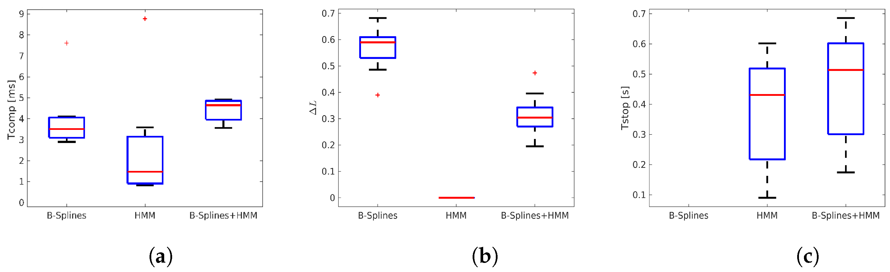
• The average computation time for a single iteration $T_{comp}$.
• The normalized average path deviation $\Delta L$, calculated as the mean deviation of the traveled distance normalized over the nominal path.
• The average stop time, $T_{stop}$, calculated as the average time taken for parameter $\alpha$ in (9) to reach zero (i.e., stop the robot) once the hand collision was perceived.
• The success rate, $\rho$, defined as the percentage of cases where the distance did not go below a given safety threshold (equal to 10 cm in our experiments) compared to the total number of situations where an incipient collision was detected.

Figure 7 displays snapshots of the real experiments conducted on the robot to test the B-spline–HMM-based controller.

4.2. Results

In Figure 8 and

Table 1. Validation tests results in terms of average computation time for single iteration $T_{comp}$, normalized average path deviation $\Delta L$, average stop time $T_{stop}$, and success rate $\rho$.

	${\mathit{T}}_{\mathit{c}\mathit{o}\mathit{m}\mathit{p}}$ (ms)	$\mathbf{\Delta }\mathit{L}$	${\mathit{T}}_{\mathit{s}\mathit{t}\mathit{o}\mathit{p}}$ (s)	$\mathit{\rho }$
B-spline	3.515 ± 1.53	0.590 ± 0.08	/	77.97%
HMM	1.480 ± 2.70	0.000 ± 0.00	0.431 ± 0.01	89.66%
B-spline+HMM	4.649 ± 0.55	0.304 ± 0.07	0.514 ± 0.01	94.41%

, we report the results of the experiments that are discussed further in the following paragraphs, while in Figure 9, we present a comparison of the trajectory of the hand recorded and virtually reproduced in three different tests using B-spline, HMM, and B-spline–HMM-based controllers. The XY projections on the right show path modifications, while temporal modulation along the time axis is observed. To assess the performance of the controllers under different scenarios, several experiments were conducted where the robot executed the same task repeatedly. These experiments involved varying parameters such as $\xi$ (balance between trajectory and symbolic control), task execution speed, and acceleration.

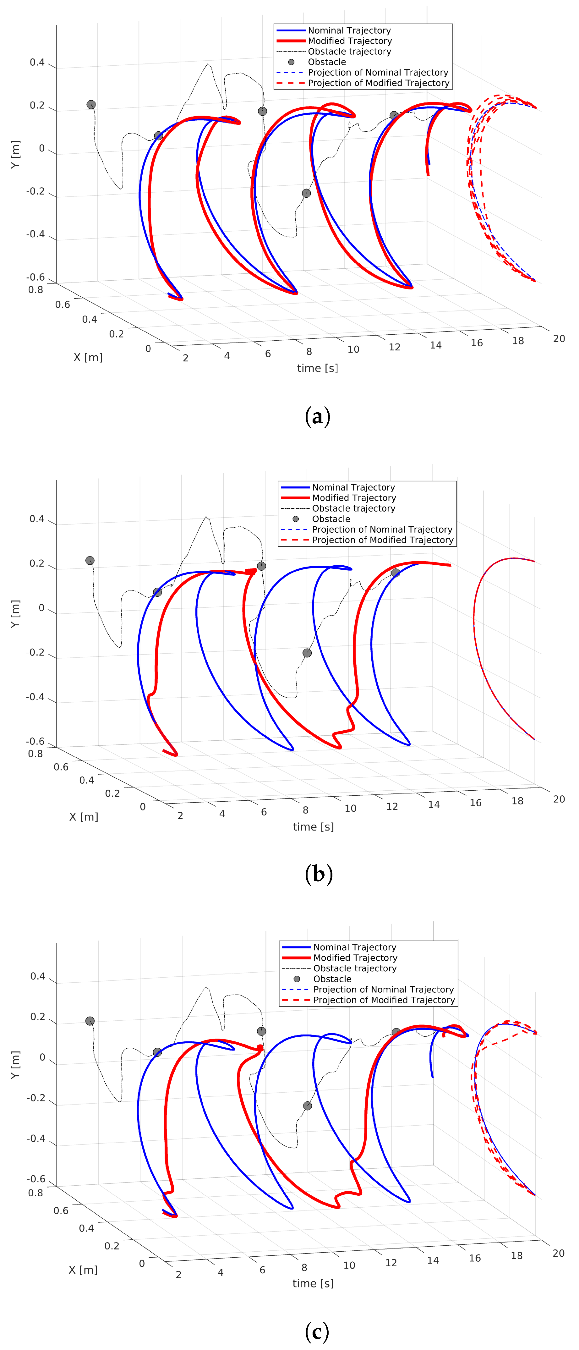
4.2.1. Controller at Trajectory Level Only ($\xi =1.0$)

In this test, the controller operated solely at the trajectory level, with $\xi =1.0$. The average computation time for a single iteration was $T_{comp}=3.515$ ms. Across six different experiments, the robot encountered a total of 59 possible collision situations. The success rate ($\rho$) achieved was 77.97%, and the normalized average path deviation ($\Delta L$) was $0.590$. Since the controller only focused on spatial control without temporal modulation, no value of $T_{stop}$ was reported as the robot never stops.

4.2.2. Controller at Symbolic Level Only ($\xi =0.0$)

In the second test, the controller operated exclusively at the symbolic level, with $\xi =0.0$. It employed an HMM with an observation space described by a GMM with seven components. The average computation time for a single iteration was $T_{comp}=1.480$ ms. Across five different experiments, the robot faced 58 possible collision situations. The success rate ($\rho$) achieved was 89.66%, with an average stop time ($T_{stop}$) of $0.431$ s and $\Delta L=0.0$ since no spatial controller was implemented.

4.2.3. Controller at Both Trajectory and Symbolic Levels ($\xi =0.5$)

In the final validation test, the task was encoded using a control at both the trajectory and symbolic levels, with $\xi =0.5$. Similar configuration parameters as the previous tests were maintained. The average computation time for a single iteration was $T_{comp}=4.649$ ms, which was slightly higher than the previous cases but still met real-time requirements within 16 ms [3,4]. Across 10 different experiments, the robot encountered 143 possible collision situations. The success rate ($\rho$) achieved was 94.41%, with a normalized average path deviation ($\Delta L$) of 0.304 m and an average stop time ($T_{stop}$) of $0.514$ s.

4.2.4. Performance Analysis

In the first scenario with only B-spline modification as the control ($\xi =1.0$), the performance was relatively poor ($\rho =77.97\%$). The controller lacked velocity control, leading to difficulties in rapidly modifying the robot’s path to avoid collisions. Additionally, tuning $(m_i,b_i,k_i)$ parameters could tighten or relax $\Delta L$, but the controller’s overall performance was unsatisfactory due to the absence of temporal modulation. Similarly, in the controller employing only HMM control ($\xi =0.0$), performance was improved compared to B-spline control ($\rho =89.66\%$). However, this controller’s behavior was inadequate when the operator’s hand moved towards the robot. By integrating the B-spline and HMM controllers, the combined B-spline–HMM controller achieved a higher success rate ($\rho =94.41\%$). Although the average stop time ($T_{stop}$) was higher than the HMM controller alone, real-time requirements were still satisfied [3,4] and the B-spline–HMM controller consistently slowed down and modified the robot’s path until the safety distance was maintained before stopping completely. The normalized average path deviation ($\Delta L$) was lower compared to the trajectory level only controller, as the robot now reduced its velocity towards the hand and stopped before any collisions. This feature was critical in avoiding potential singular configurations that could occur with the B-spline controller alone.

5. Conclusions and Future Work

In this paper, a novel framework for obstacle avoidance applications is introduced. After several real-world experiments, we believe that our methodology is suitable for human–robot shared environments, meeting real-time requirements for safe cooperation. The proposed work introduces a motion planning algorithm that can be adapted to different scenarios with moving and static obstacles, achieving a success rate of $94.41\%$. By combining the trajectory and symbolic domains, our framework can smoothly adapt the Cartesian path and slow down the execution of the task in the proximity of a human operator. Moreover, by associating a dynamical system with each control point, the controller autonomously resets to its original task, and while using the HMM, the robot never stops after overtaking the operator’s hand, ensuring correct and complete task execution. Clarifications should be made w.r.t. to all the situations where a collision occurs. The B-spline–HMM architectures ensures safety as long as the position of the obstacle is known. A positive feature of our controller is that the robot is halted every time the obstacle is too close, strongly reducing the impact in case of a collision.

Future work might involve the use of multiple cameras to span over a wider workspace and improve the detection of obstacles, no longer limited to the operator’s hand. Triangulation techniques could be, in this case, a solution to enhance the marker measurement’s precision, as during experiments, we registered an accuracy sometimes lower than 4 cm. Moreover, it could be desirable to improve the algorithm that predicts the motion of moving obstacles and operators to obtain a larger time horizon, more consistent with a smooth obstacle avoidance application. While the algorithm was validated on one task, additional experiments and validations involving various test scenarios are needed. Preferably, these tests should apply the algorithm to the joint space, including new techniques for obstacle–robot distance measurements, that might be extended to the whole body of the manipulator rather than just the end effector.

References

- Khansari-Zadeh, S.M.; Khatib, O. Learning Potential Functions from Human Demonstrations with Encapsulated Dynamic and Compliant Behaviors. Auton. Robot. 2017, 41, 45–69. [Google Scholar] [CrossRef]
- Scalera, L.; Giusti, A.; Vidoni, R.; Gasparetto, A. Enhancing fluency and productivity in human-robot collaboration through online scaling of dynamic safety zones. Int. J. Adv. Manuf. Technol. 2022, 121, 6783–6798. [Google Scholar] [CrossRef]
- Liu, H.; Qu, D.; Xu, F.; Du, Z.; Jia, K.; Song, J.; Liu, M. Real-Time and Efficient Collision Avoidance Planning Approach for Safe Human-Robot Interaction. J. Intell. Robot. Syst. 2022, 105, 93. [Google Scholar] [CrossRef]
- Merckaert, K.; Convens, B.; Wu, C.-J.; Roncone, A.; Nicotra, M.M.; Vanderborght, B. Real-Time Motion Control of Robotic Manipulators for Safe Human-Robot Coexistence. Robotics 2022, 73, 102223. [Google Scholar] [CrossRef]
- Chiaravalli, D.; Califano, F.; Biagiotti, L.; De Gregorio, D.; Melchiorri, C. Physical-Consistent Behavior Embodied in B-Spline Curves for Robot Path Planning. IFAC-PapersOnLine 2018, 51, 306–311. [Google Scholar] [CrossRef]
- Kanazawa, A.; Kinugawa, J.; Kosuge, K. Adaptive Motion Planning for a Collaborative Robot Based on Prediction Uncertainty to Enhance Human Safety and Work Efficiency. IEEE Trans. Robot. 2019, 35, 817–832. [Google Scholar] [CrossRef]
- Zanchettin, A.M.; Ceriani, N.M.; Rocco, P.; Ding, H.; Matthias, B. Safety in Human-Robot Collaborative Manufacturing Environments: Metrics and Control. IEEE Trans. Autom. Sci. Eng. 2015, 13, 882–893. [Google Scholar] [CrossRef]
- Zucker, M.; Ratliff, N.; Dragan, A.D.; Pivtoraiko, M.; Klingensmith, M.; Dellin, C.M.; Bagnell, J.A.; Srinivasa, S.S. Chomp: Covariant Hamiltonian Optimization for Motion Planning. Int. J. Robot. Res. 2013, 32, 1164–1193. [Google Scholar] [CrossRef]
- Yang, C.; Sue, G.N.; Li, Z.; Yang, L.; Shen, H.; Chi, Y.; Rai, A.; Zeng, J.; Sreenath, K. Collaborative Navigation and Manipulation of a Cable-Towed Load by Multiple Quadrupedal Robots. IEEE Robot. Autom. Lett. 2022, 7, 10041–10048. [Google Scholar] [CrossRef]
- Mukadam, M.; Dong, J.; Yan, X.; Dellaert, F.; Boots, B. Continuous-Time Gaussian Process Motion Planning via Probabilistic Inference. Int. J. Robot. Res. 2018, 37, 1319–1340. [Google Scholar] [CrossRef]
- Toussaint, M.; Goerick, C. A Bayesian View on Motor Control and Planning. In From Motor Learning to Interaction Learning in Robots; Springer: Berlin/Heidelberg, Germany, 2010; pp. 227–252. [Google Scholar] [CrossRef]
- Fisac, J.F.; Bajcsy, A.; Herbert, S.L.; Fridovich-Keil, D.; Wang, S.; Tomlin, C.J.; Dragan, A.D. Probabilistically Safe Robot Planning with Confidence-Based Human Predictions. arXiv 2018, arXiv:1806.00109. [Google Scholar]
- Calinon, S.; Guenter, F.; Billard, A. On Learning, Representing, and Generalizing a Task in a Humanoid Robot. IEEE Trans. Syst. Man Cybern. Part Cybern. 2007, 37, 286–298. [Google Scholar] [CrossRef]
- Kavraki, L.E.; LaValle, S.M. Motion Planning. In Springer Handbook of Robotics; Springer: Berlin/Heidelberg, Germany, 2016; pp. 139–162. [Google Scholar] [CrossRef]
- Jankowski, J.; Brudermüller, L.; Hawes, N.; Calinon, S. VP-STO: Via-Point-Based Stochastic Trajectory Optimization for Reactive Robot Behavior. arXiv 2022, arXiv:2210.04067. [Google Scholar]
- Han, D.; Nie, H.; Chen, J.; Chen, M. Dynamic Obstacle Avoidance for Manipulators Using Distance Calculation and Discrete Detection. Robot. Comput.-Integr. Manuf. 2018, 49, 98–104. [Google Scholar] [CrossRef]
- Khatib, O. Real-time Obstacle Avoidance for Manipulators and Mobile Robots. In Proceedings of the 1985 IEEE International Conference on Robotics and Automation, St. Louis, MO, USA, 25–28 March 1985; Volume 2, pp. 500–505. [Google Scholar] [CrossRef]
- Quinlan, S.; Khatib, O. Elastic Bands: Connecting Path Planning and Control. In Proceedings of the [1993] Proceedings IEEE International Conference on Robotics and Automation, Atlanta, GA, USA, 2–6 May 1993; pp. 802–807. [Google Scholar] [CrossRef]
- Flacco, F.; Kröger, T.; Luca, A.D.; Khatib, O. A Depth Space Approach to Human-Robot Collision Avoidance. In Proceedings of the 2012 IEEE International Conference on Robotics and Automation, St. Paul, MN, USA, 14–18 May 2012; pp. 338–345. [Google Scholar] [CrossRef]
- Secil, S.; Ozkan, M. A collision-free path planning method for industrial robot manipulators considering safe human-robot interaction. Intell. Serv. Robot. 2023, 16, 323–359. [Google Scholar] [CrossRef]
- ISO/TS 15066; Robots and Robotic Devices—Collaborative Robots. International Organization for Standardization: Geneva, Switzerland, 2016.
- Rosenstrauch, M.J.; Pannen, T.J.; Krüger, J. Human Robot Collaboration—Using Kinect v2 for ISO/TS 15066 Speed and Separation Monitoring. Procedia CIRP 2018, 76, 183–186. [Google Scholar] [CrossRef]
- Lagomarsino, M.; Lorenzini, M.; Constable, M.D.; De Momi, E.; Becchio, C.; Ajoudani, A. Maximising Coefficiency of Human-Robot Handovers through Reinforcement Learning. IEEE Robot. Autom. Lett. 2023, 8, 4378–4385. [Google Scholar] [CrossRef]
- Calinon, S.; Billard, A.; Dillmann, R.; Schaal, S. Robot Programming by Demonstration. In Springer Handbook of Robotics; Siciliano, B., Khatib, O., Eds.; Springer: Berlin/Heidelberg, Germany, 2008. [Google Scholar] [CrossRef]
- Biagiotti, L.; Melchiorri, C. Trajectory Planning for Automatic Machines and Robots; Springer Science & Business Media: Berlin/Heidelberg, Germany, 2008. [Google Scholar] [CrossRef]
- Pentland, A.; Liu, A. Modeling and Prediction of Human Behavior. Neural Comput. 1999, 11, 229–242. [Google Scholar] [CrossRef]
- Hovland, G.E.; Sikka, P.; McCarragher, B.J. Skill Acquisition from Human Demonstration Using a Hidden Markov Model. In Proceedings of the IEEE International Conference on Robotics and Automation, Minneapolis, MN, USA, 22–28 April 1996; Volume 3, pp. 2706–2711. [Google Scholar] [CrossRef]
- Roveda, L.; Magni, M.; Cantoni, M.; Piga, D.; Bucca, G. Human-Robot Collaboration in Sensorless Assembly Task Learning Enhanced by Uncertainties Adaptation via Bayesian Optimization. Robot. Auton. Syst. 2021, 136, 103711. [Google Scholar] [CrossRef]
- Biagiotti, L.; Melchiorri, C. Online Trajectory Planning and Filtering for Robotic Applications via B-Spline Smoothing Filters. In Proceedings of the 2013 IEEE/RSJ International Conference on Intelligent Robots and Systems, Tokyo, Japan, 3–7 November 2013; pp. 5668–5673. [Google Scholar] [CrossRef]
- Sayols, N.; Sozzi, A.; Piccinelli, N.; Hernansanz, A.; Casals, A.; Bonfè, M.; Muradore, R. Global/Local Motion Planning Based on Dynamic Trajectory Reconfiguration and Dynamical Systems for Autonomous Surgical Robots. In Proceedings of the 2020 IEEE International Conference on Robotics and Automation (ICRA), Paris, France, 31 May–31 August 2020; pp. 8483–8489. [Google Scholar] [CrossRef]
- Jurafsky, D.; Martin, J. Speech and Language Processing: An Introduction to Natural Language Processing, Computational Linguistics, and Speech Recognition; Prentice Hall PTR: Upper Saddle River, NJ, USA, 2008; Volume 2, Available online: https://dl.acm.org/doi/10.5555/555733 (accessed on 9 August 2023).
- Mongillo, G.; Deneve, S. Online Learning with Hidden Markov Models. Neural Comput. 2008, 20, 1706–1716. [Google Scholar] [CrossRef]
- Vasquez, D.; Fraichard, T.; Laugier, C. Incremental Learning of Statistical Motion Patterns with Growing Hidden Markov Models. IEEE Trans. Intell. Transp. Syst. 2009, 10, 403–416. [Google Scholar] [CrossRef]
- Walter, M.; Psarrou, A.; Psarrou, R.; Gong, S. Learning Prior and Observation Augmented Density Models for Behaviour Recognition. In Proceedings of the BMVC 1999—British Machine Vision Conference 1999, Nottingham, UK, 13–16 September 1999. [Google Scholar]
- Meuter, M.; Iurgel, U.; Park, S.-B.; Kummert, A. The Unscented Kalman Filter for Pedestrian Tracking from a Moving Host. In Proceedings of the 2008 IEEE Intelligent Vehicles Symposium, Eindhoven, The Netherlands, 4–6 June 2008; pp. 37–42. [Google Scholar] [CrossRef]
- Wiest, J.; Höffken, M.; Kreßel, U.; Dietmayer, K. Probabilistic Trajectory Prediction with Gaussian Mixture Models. In Proceedings of the 2012 IEEE Intelligent Vehicles Symposium, Madrid, Spain, 3–7 June 2012; pp. 141–146. [Google Scholar] [CrossRef]
- Gaz, C.; Cognetti, M.; Oliva, A.; Robuffo Giordano, P.; De Luca, A. Dynamic Identification of the Franka Emika Panda Robot with Retrieval of Feasible Parameters Using Penalty-Based Optimization. IEEE Robot. Autom. Lett. 2019, 4, 4147–4154. [Google Scholar] [CrossRef]
- Quigley, M.; Gerkey, B.; Smart, W.D. Programming Robots with ROS: A Practical Introduction to the Robot Operating System; O’Reilly Media, Inc.: Sebastopol, CA, USA, 2015. [Google Scholar]
- Garrido-Jurado, S.; Muñoz-Salinas, R.; Madrid-Cuevas, F.J.; Marín-Jiménez, M.J. Automatic Generation and Detection of Highly Reliable Fiducial Markers Under Occlusion. Pattern Recognit. 2014, 47, 2280–2292. [Google Scholar] [CrossRef]
- Kohler, M. Using the Kalman Filter to Track Human Interactive Motion: Modelling and Initialization of the Kalman Filter for Translational Motion; Citeseer: Pennsylvania, PA, USA, 1997. [Google Scholar]
- Julier, S.J.; Uhlmann, J.K. New Extension of the Kalman Filter to Nonlinear Systems. In Proceedings of the Signal Processing, Sensor Fusion, and Target Recognition VI, Orlando, FL, USA, 21–24 April 1997; Volume 3068, pp. 182–193. [Google Scholar] [CrossRef]