Modal Kinematic Analysis of a Parallel Kinematic Robot with Low-Stiffness Transmissions

Abstract

Several industrial robotic applications that require high speed or high stiffness-to-inertia ratios use parallel kinematic robots. In the cases where the critical point of the application is the speed, the compliance of the main mechanical transmissions placed between the actuators and the parallel kinematic structure can be significantly higher than that of the parallel kinematic structure itself. This paper deals with this kind of system, where the overall performance depends on the maximum speed and on the dynamic behavior. Our research proposes a new approach for the investigation of the modes of vibration of the end-effector placed on the robot structure for a system where the transmission’s compliance is not negligible in relation to the flexibility of the parallel kinematic structure. The approach considers the kinematic and dynamic coupling due to the parallel kinematic structure, the system’s mass distribution and the transmission’s stiffness. In the literature, several papers deal with the dynamic vibration analysis of parallel robots. Some of these also consider the transmissions between the motors and the actuated joints. However, these works mainly deal with the modal analysis of the robot’s mechanical structure or the displacement analysis of the transmission’s effects on the positioning error of the end-effector. The discussion of the proposed approach takes into consideration a linear delta robot. The results show that the system’s natural frequencies and the directions of the end-effector’s modal displacements strongly depend on its position in the working space.

1. Introduction

Parallel robots are Parallel Kinematics Machines (PKM) which have been investigated for a long time, as demonstrated by some key papers [1,2,3]. The parallel kinematic configuration gives to these robotic systems a high stiffness/inertia ratio. This characteristic is due to closed kinematic chains, where some members are mainly subject to axial loads; hence, these links can be designed to be slender and light without the risk of decreasing the system’s overall stiffness. Moreover, the parallel kinematic configuration allows the positioning of the driving motors on the fixed frame of the robot, reducing, therefore, the moving masses [4,5].

The linear delta kinematic configuration [3] is characterized by linear axes instead of the rotary ones used within the well-known classical Delta configuration [1,2]. As a result, for this configuration, the working volume is spatially extended along a direction whose length depends only on the length of the linear axes. Applications in the industrial field requiring high speed and working volume extended along a direction can use linear delta robots designed with a suitable transmission that on one hand permits high linear speed and on the other has low inertia. This configuration is suitable for the primary packaging station of a production line or for transferring production goods between two lines. Linear transmissions based on a timing belt are an interesting solution due to the low mass, high speed, long travel length and low cost, especially if compared with other kinds of linear transmissions, such as ball-screws.

It should be moreover remarked that the overall performance of the system depends not only on the kinematic structure of the manipulator, but also on the characteristics of transmissions between motors and joints; hence, in order to achieve the expected system performance, the synthesis requires a synergistic design approach [6].

Despite the attractive characteristics of a belt transmission from the inertial point of view, it is also a well-known intrinsically deformable device that introduces significant flexibility between motors and driven joints. Several researchers have investigated belt transmissions for many years under several aspects. Some authors defined a methodology for the estimation of the characteristic parameters of a linear belt drive, considering lumped parameter modeling, mainly for control purpose [7]. Other authors focused their attention on the acoustic radiation of a timing belt due to its vibrations. Such dynamic behavior was investigated by means of a numerical multi-body model [8]. As far as modeling is concerned, many authors developed numerical models of timing belts, taking into consideration also the interaction between the belt and pulley [9,10,11]. Other recent works also focused on the influence of the tensioner on the dynamic behavior of the belt [12,13], while other papers dealt with new issues concerning the usage of oval pulleys in belt transmissions [14,15]. As confirmation of the researcher’s interest in the dynamic behavior of timing belts, there is also an interesting review on the methodologies for modeling and analysis of the axial and torsional vibration of these kinds of transmissions [16].

Regarding the dynamics of a parallel kinematics robot, many works can be found in the literature where the modal analysis of the system is performed, but only taking into consideration the robotic system and not the contribution due to the transmissions’ stiffness. In this context, some authors performed the modal analysis, developing the models by means of a commercial software [17,18,19,20], while other authors developed their own model [21,22,23,24], sometimes with the aim to investigate the low-order dynamics of the system [25]; in all these cases, nothing about the transmission is taken into consideration.

In the literature, papers focusing on both the robotic system and on the transmission can be found. However, they generally concern the definition of control algorithms for the suppression of vibrations [26,27], the estimation of the system’s parameters [28], or the definition of the positioning error in the workspace [29,30].

Our research is related to investigating the dynamic vibration behavior of parallel kinematics robots, where the mechanical transmissions have lower stiffness than the one of the parallel kinematic structure. This approach is quite different from the methodologies detailed in the previously cited works. In particular, we are interested in the overall system, transmissions included, focusing on the influence of the transmissions’ stiffness on the natural frequencies and the mode shapes of the parallel robot.

The main contribution of our paper is to highlight, taking into consideration also the transmissions and their stiffness, how the modes of vibration of the belt transmissions’ carriages, which depend on the mass distribution within the system and on the coupling effect due to the parallel kinematic chains, are reflected to the end-effector as a function of its position within the workspace. The results are the end-effector’s modal displacements’ directions due to the system’s characteristics. Moreover, these results are a function of the end-effector position in the workspace. For this reason, we have named our approach “Modal Kinematic Analysis”.

The paper takes into consideration a 3 d.o.f. linear delta produced by the Italian company Mechatronics and Dynamic Devices s.r.l. [31]. This device has linear belt transmissions on which we have already carried out some experimental activities, showing the influence of the belt transmissions’ stiffness on the dynamics of the overall system [32]. As previously mentioned, the stiffness of the parallel kinematic part is higher than the rigidity of the belts; this is why we have modeled the parallel kinematic part as being rigid, considering the belt transmissions to be the only deformable elements. Regarding the transmissions, we already highlighted that we are not interested in analyzing specific aspects, such as acoustic emissions, due to the belt’s vibration or the contact between the belt and pulley. Moreover, in the case of a linear drive system that moves a carriage with a mass significantly higher than the belt’s mass, the latter can be neglected; hence, the transmission can be modeled as the lumped stiffnesses, one for each part of the belt, changing with the configuration of the transmission, i.e., changing with the carriages positions.

2. Materials and Methods

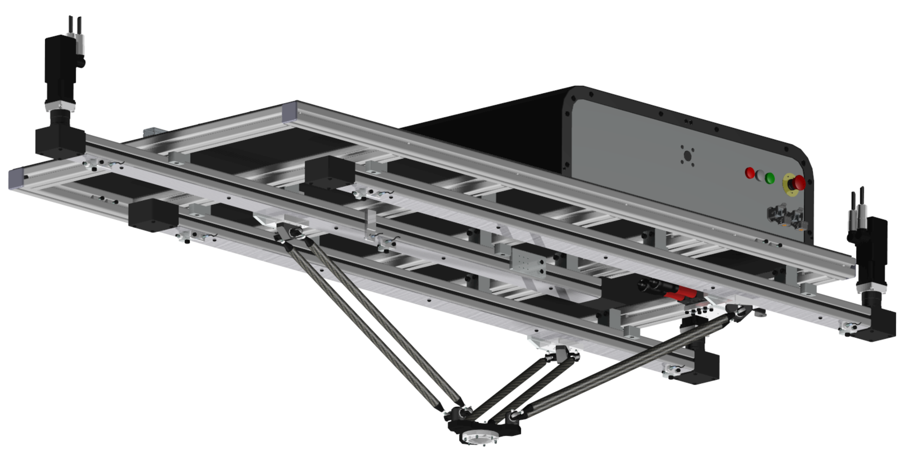
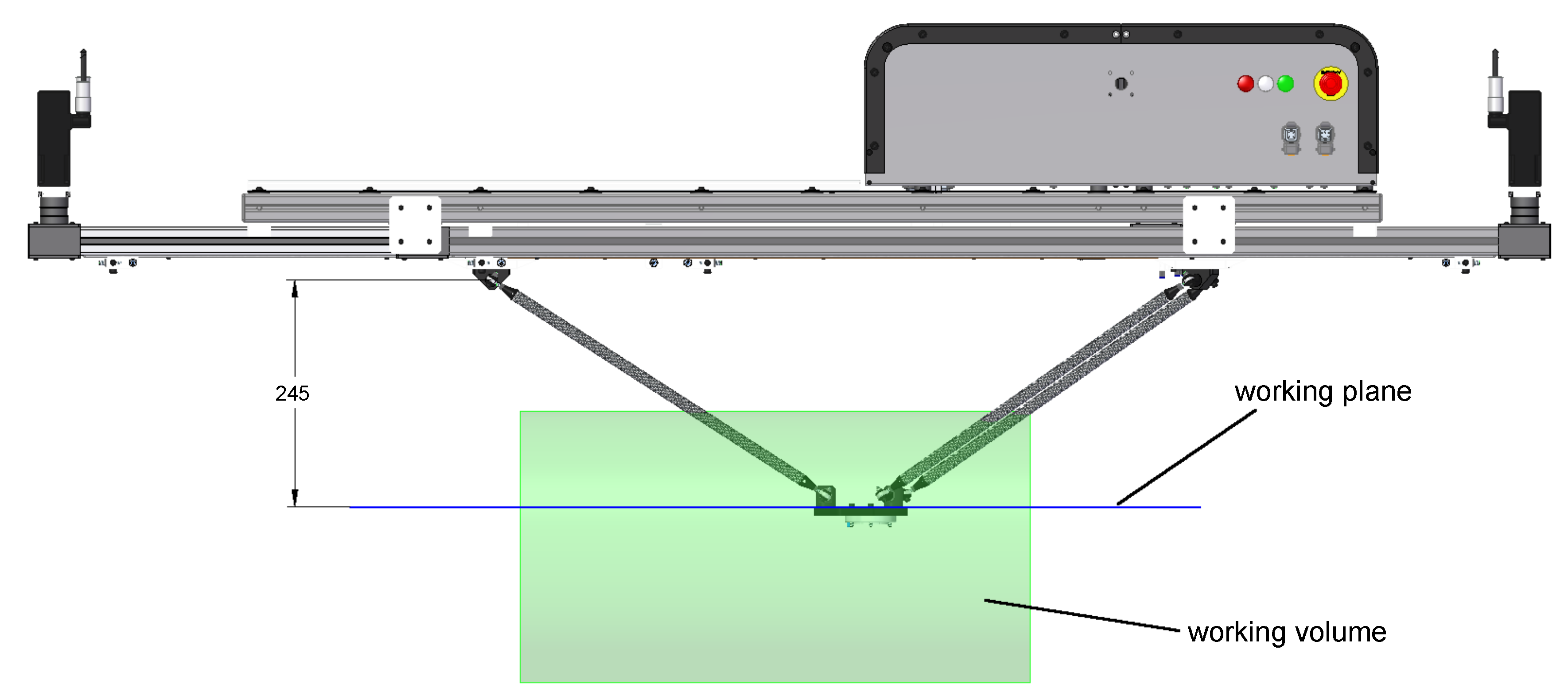
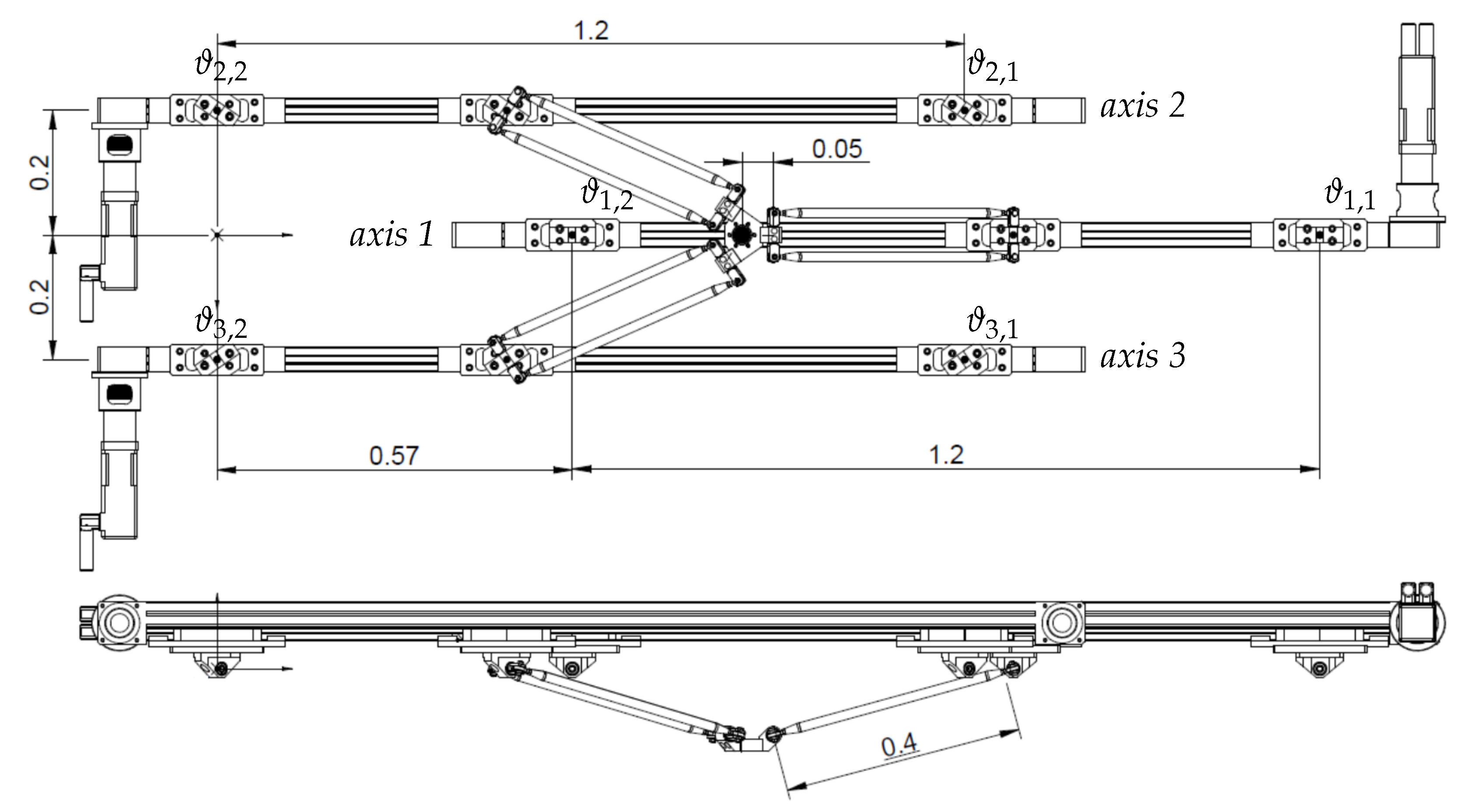
2.1. The Parallel Robot under Analysis

The parallel robot on which we have applied our “Modal Kinematic Analysis” approach is a 3 d.o.f. parallel kinematic machine produced by the Italian company Mechatronics and Dynamic Devices s.r.l. [31] that is characterized by the typical linear delta kinematic configuration.

Figure 1 and Figure 2 present the linear delta, whose main characteristics are the following:

• The three linear axes are parallel.
• Each linear axis is composed of a linear belt transmission. The belt is a HTD-5 characterized by a 15 mm width and a specific stiffness (or stiffness per unit of length and unit of width) of $k_{sp}$ = 2.42 × 10⁶ N/m.
• The system is driven by means of brushless motors, characterized by a nominal torque of 0.7 Nm; a maximum velocity of 10,000 rpm; and a rotor inertia of 0.017 × 10⁻³ kg·m².
• The motors are connected to the driven pulley of the linear belt transmission by means of a planetary gearbox characterized by a reduction ratio equal to 10.
• The maximum axis stroke is 1.2 m.
• The distance $l_r$ between axes is 200 mm.
• The length $l_d$ of the links connecting the carriages to the end-effector is 400 mm.

The constraints between the links and, respectively, the carriages and the mobile platform are realized by means of universal joints, highlighted in blue for the carriages and in red for the mobile platform in Figure 3. Hence, each link is composed of two rods realizing a four bar linkage with a parallelogram configuration.

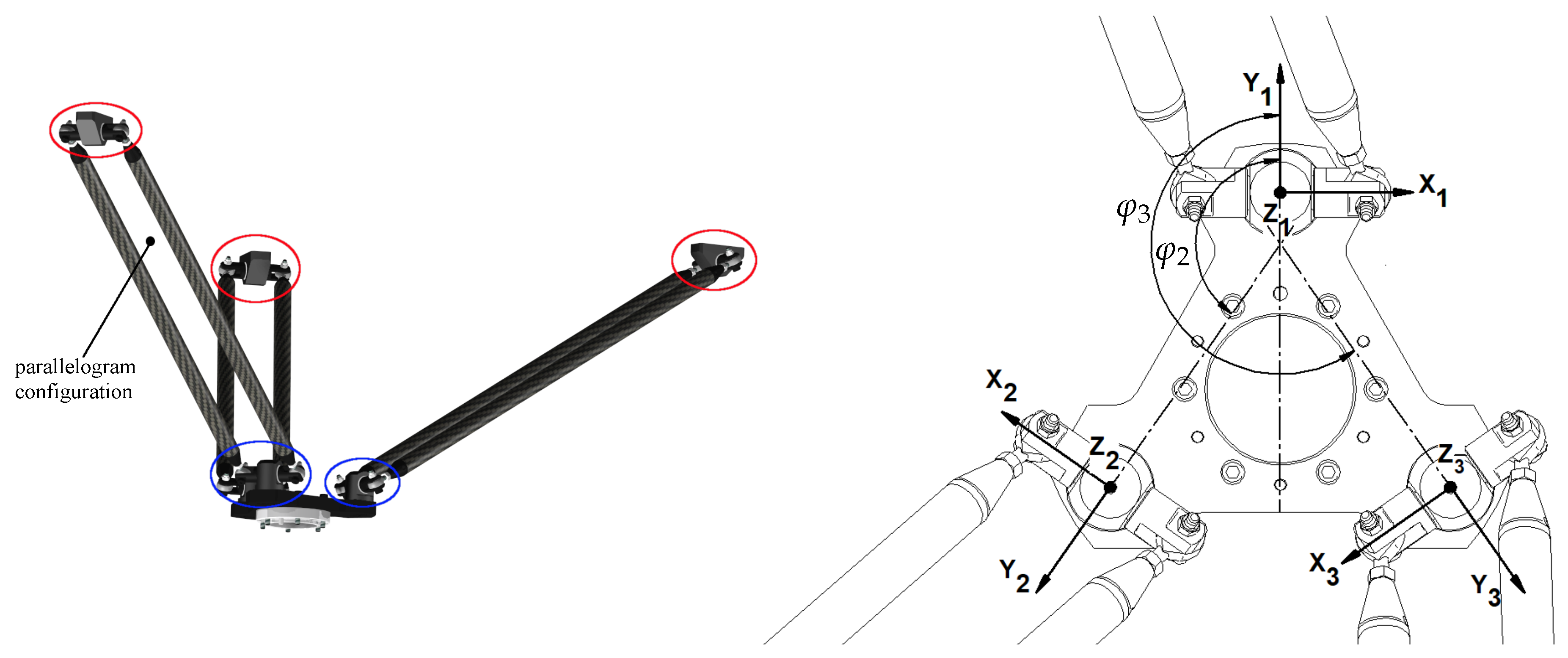
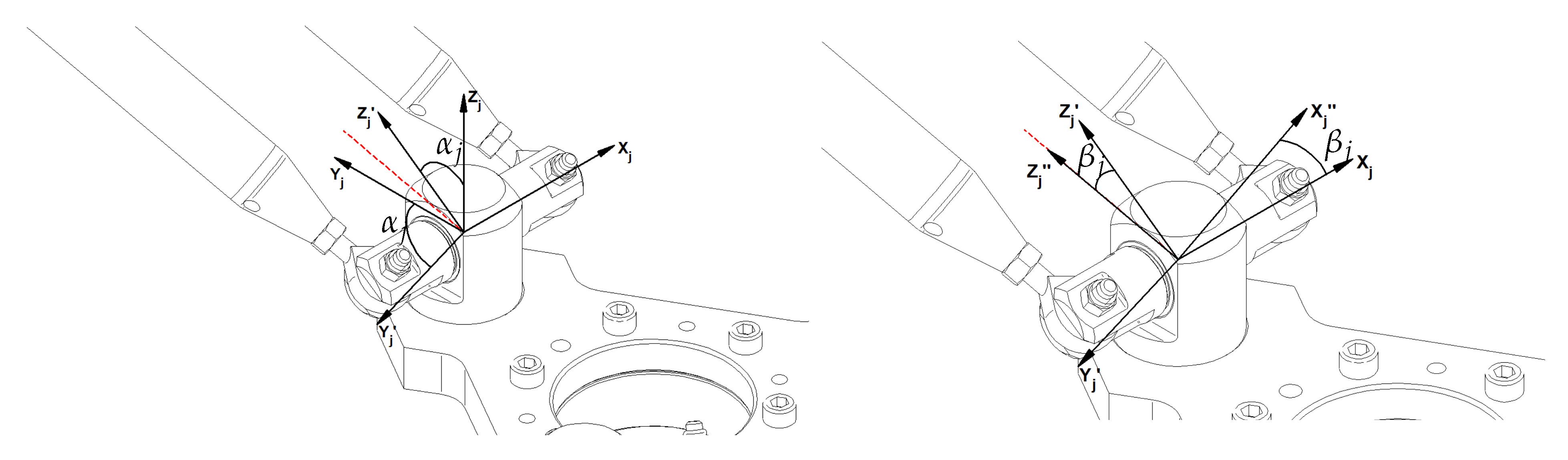
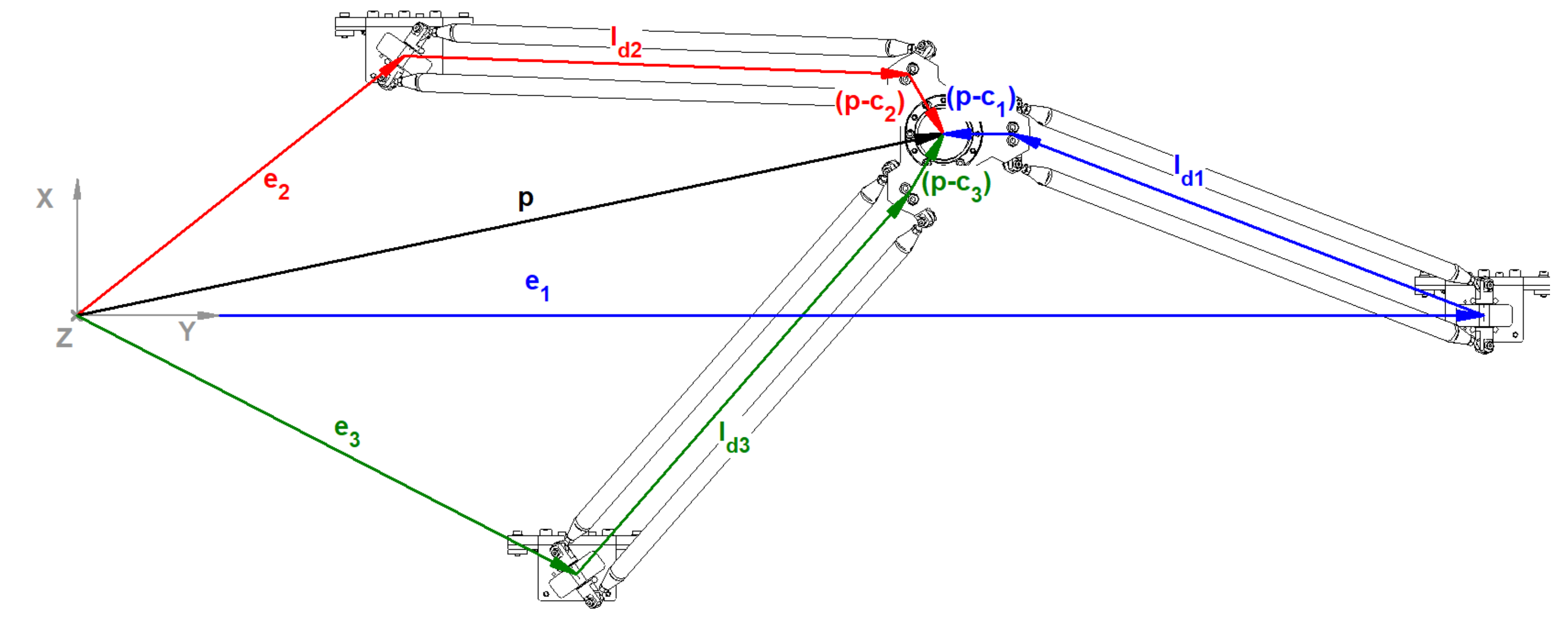
2.2. Kinematics and Dynamics of the Parallel Kinematic Part

This section presents the model for the kinematics and the dynamics of the parallel kinematic part of the manipulator. This part has very high stiffness and low weight due to the carbon fiber composite material of the rods. For these reasons, it is possible to say that the flexibility of the parallel kinematic part can be considered negligible with respect to the compliance of the linear belt transmissions. This subsystem can be thus modeled as being composed of rigid bodies, whereas the only flexible elements are the transmissions. Moreover, the belt’s mass is negligible with respect to the carriages mass; accordingly, we neglect the inertial contributions of the belt, and simply model its stiffness using configuration-dependent lumped parameters.

The rigid structure of the manipulator is responsible not only for the dynamic coupling between the linear axes, but also for the overall mass distribution of the system; the rigid-body kinematics and dynamics of this subsystem—composed of the mobile platform, of the distal links and of the trucks—must, therefore, be thoroughly accounted for.

The kinematics of the manipulator are largely analogous to those of the Delta robot designed by Reymond Clavel and analyzed, for example, in [1,2]; as such, this mechanical structure results in a mobile platform with three translational degrees of freedom [3]. Figure 2 shows the reference frame with respect to which the end effector’s position is measured, while Figure 3 depicts three sets of local coordinates useful to completely describe the kinematics of the parallel bar linkages.

The angular positions ${\phi }_j^{}$, $j=1,2,3$ of the universal joints that connect the distal rods to the platform are also shown in Figure 3. The free coordinates $x_1$, $x_2$ and $x_3$ that govern the kinematics of the manipulator are those relative to the longitudinal displacement of the three trucks. Given the geometric parameter $l_r$ that defines the distance between two adjacent linear guides, the truck positions ${\mathit{e}}_{\mathit{j}}^{}$ are trivially expressed as functions of $x_j$:

$${\mathit{e}}_{\mathbf{1}}^{}=\left[\begin{array}{c}{x}_1\\ 0\\ 0\end{array}\right],{\mathit{e}}_{\mathbf{2}}^{}=\left[\begin{array}{c}{x}_2\\ -l_r,\\ 0\end{array}\right],{\mathit{e}}_{\mathbf{3}}^{}=\left[\begin{array}{c}{x}_3\\ l_r,\\ 0\end{array}\right].$$

(1)

The direct and inverse functions between these quantities and the center point $\mathit{p}$ of the moving platform must furthermore be determined. The chief relationships that allow to do so are the vector loop equations written for each kinematic chain:

$$\begin{array}{cc}\hfill {\mathit{e}}_{\mathit{j}}^{}+{\mathit{l}}_{\mathit{d},\mathit{j}}+(\mathit{p}-{\mathit{c}}_{\mathit{j}}^{})=\mathit{p}& \forall j\in [1,2,3].\end{array}$$

(2)

In Equation (2), ${\mathit{l}}_{\mathit{d},\mathit{j}}$ is the vector pointing from the $j^{th}$ truck ${\mathit{e}}_{\mathit{j}}^{}$ to the position ${\mathit{c}}_{\mathit{j}}^{}$ of the $j^{th}$ platform universal joint constraint, while the difference $(\mathit{p}-{\mathit{c}}_{\mathit{j}}^{})$ is a constant vector entirely determined by the geometry of the moving platform.

The vector loop equations, whose geometric meaning is depicted in Figure 4, must be satisfied for every assembled configuration of the robot. To exactly enforce them when the truck position vectors ${\mathit{e}}_{\mathit{j}}^{}$ are known, it is sufficient to intersect three spheres of radius $l_d$ and centered in the points,

$$\begin{array}{c}\hfill {\mathit{s}}_{\mathit{j}}={\mathit{e}}_{\mathit{j}}^{}+(\mathit{p}-{\mathit{c}}_{\mathit{j}}^{});\end{array}$$

(3)

indeed, the intersection point coincides with the admissible $\mathit{p}$, from which the constraint positions ${\mathit{c}}_{\mathit{j}}^{}$ can be then found.

On the other hand, if $\mathit{p}$ is given the points ${\mathit{c}}_{\mathit{j}}^{}$ can be immediately determined; the intersection of the sphere of radius $l_d$ and center ${\mathit{c}}_{\mathit{j}}^{}$ with the segment generated by the $j^{th}$ linear guide allows then the determination of ${\mathit{e}}_{\mathit{j}}^{}$ (and $x_j$) that satisfy the vector loop equations.

Other positional quantities of interest are the centers of mass of the distal linkages and the Euler angles describing the rotation of the linkage rods. Since the two rods of each linkage are constrained to perform the same motion, the kinematics of the entire distal link can be abstracted to those of its center-line.

Given that each distal rod is a slender, axially symmetric body, the position ${\mathit{d}}_{\mathit{j}}^{}$ of the center of mass of the $j^{th}$ linkage can be expressed as a weighted average of the constraint and carriage position.

$$\begin{array}{c}\hfill {\mathit{d}}_{\mathit{j}}^{}={\displaystyle \frac{W_c{\mathit{c}}_{\mathit{j}}^{}+W_t{\mathit{e}}_{\mathit{j}}^{}}{W_c+W_t}},\end{array}$$

(4)

where $W_c$ is the weight of the universal joint and $W_t$ is the weight of the truck.

A physically meaningful description of the distal link rotation must take into account the actual configuration of the universal joint connecting each rod pair to the end-effector. With reference to Figure 5, where the red dashed line represents the direction of the generic link j, the most straightforward solution involves a joint allowing a rotation of the rod pair first around the local x-axis by an angle ${\alpha }_j$, and then around the rotated local y${}^{\prime }$-axis by an angle ${\beta }_j$. The third Euler angle ${\gamma }_j$ around the local z${}^{″}$-axis, directed as the distal rod itself, is kinematically constrained to be equal to zero.

Given the vector

$$\begin{array}{c}\hfill {\mathit{u}}_{\mathit{j}}={\mathit{e}}_{\mathit{j}}^{\left[\mathit{j}\right]}-{\mathit{c}}_{\mathit{j}}^{\left[\mathit{j}\right]}\end{array}$$

(5)

expressed in the $j^{th}$ frame of reference, these angles are easily computed as:

$$\begin{array}{cc}& {\alpha }_j^{\left[j\right]}=arctan\left({\displaystyle \frac{-{\mathit{u}}_{\mathit{j},\mathbf{2}}}{{\mathit{u}}_{\mathit{j},\mathbf{3}}}}\right)\end{array}$$

(6)

$$\begin{array}{cc}& {\beta }_j^{\left[j\right]}=arcsin\left({\displaystyle \frac{{\mathit{u}}_{\mathit{j},\mathbf{1}}}{\left|\right|{\mathit{u}}_{\mathit{j}}\left|\right|}}\right)\end{array}$$

(7)

$$\begin{array}{cc}& {\gamma }_j^{\left[j\right]}=0.\end{array}$$

(8)

Additionally, the rotation matrix ${\mathit{R}}_{\mathit{d},\mathit{j}}^{\left[\mathit{j}\right]}$ of the distal link can be constructed from the Euler angles through standard formulas for the composition of elementary rotations.

As the position kinematics of the platform are described as a sequence of geometric rather than analytical operations, the Jacobian analysis must also be developed in the same vein. The first goal is to determine the Jacobian matrix relating the time derivative of the truck coordinates to the velocity of the mobile platform.

To do so, the formula for the velocity kinematics of rigid bodies can be applied to the three kinematic chains connecting the platform to the base. Recalling that the platform can only translate and therefore ${\dot{\mathit{c}}}_{\mathit{j}}^{}=\dot{\mathit{p}}$ the following equations can be written:

$$\begin{array}{cc}\hfill \dot{\mathit{p}}& ={\dot{\mathit{e}}}_{\mathbf{1}}^{}+{\omega }_{\mathbf{1}}^{}\wedge (\mathit{p}-{\mathit{e}}_{\mathbf{1}}^{})\end{array}$$

(9)

$$\begin{array}{cc}\hfill \dot{\mathit{p}}& ={\dot{\mathit{e}}}_{\mathbf{2}}^{}+{\omega }_{\mathbf{2}}^{}\wedge (\mathit{p}-{\mathit{e}}_{\mathbf{2}}^{})\end{array}$$

(10)

$$\begin{array}{cc}\hfill \dot{\mathit{p}}& ={\dot{\mathit{e}}}_{\mathbf{3}}^{}+{\omega }_{\mathbf{3}}^{}\wedge (\mathit{p}-{\mathit{e}}_{\mathbf{3}}^{}).\end{array}$$

(11)

The yet unknown distal angular velocities ${\omega }_{\mathit{j}}^{}$ can be eliminated from Equations (9) and (11) by multiplying each side by the quantity ${(\mathit{p}-{\mathit{e}}_{\mathit{j}}^{})}^{\top }$. In matrix notation:

$$\left[\begin{array}{c}{(\mathit{p}-{\mathit{e}}_{\mathbf{1}}^{})}^{\top }\\ {(\mathit{p}-{\mathit{e}}_{\mathbf{2}}^{})}^{\top }\\ {(\mathit{p}-{\mathit{e}}_{\mathbf{3}}^{})}^{\top }\end{array}\right]\dot{\mathit{p}}=\left[\begin{array}{c}{(\mathit{p}-{\mathit{e}}_{\mathbf{1}}^{})}^{\top }{\dot{\mathit{e}}}_{\mathbf{1}}^{}\\ {(\mathit{p}-{\mathit{e}}_{\mathbf{2}}^{})}^{\top }{\dot{\mathit{e}}}_{\mathbf{2}}^{}\\ {(\mathit{p}-{\mathit{e}}_{\mathbf{3}}^{})}^{\top }{\dot{\mathit{e}}}_{\mathbf{3}}^{}\end{array}\right].$$

(12)

The truck velocities can then be expressed in terms of the time derivatives of the free coordinates by highlighting the Jacobian matrices ${\mathit{D}}_{\mathit{e},\mathit{j}}^{}$ of ${\mathit{e}}_{\mathit{j}}^{}$ with respect to $\mathit{x}={\left[\begin{array}{ccc}{x}_1& x_2& x_3\end{array}\right]}^{\top }$:

$${\dot{\mathit{e}}}_{\mathbf{1}}^{}=\stackrel{{\mathit{D}}_{\mathit{e},\mathbf{1}}^{}}{\overbrace{\left[\begin{array}{ccc}0& 0& 0\\ 1& 0& 0\\ 0& 0& 0\end{array}\right]}}\dot{\mathit{x}},{\dot{\mathit{e}}}_{\mathbf{2}}^{}=\stackrel{{\mathit{D}}_{\mathit{e},\mathbf{2}}^{}}{\overbrace{\left[\begin{array}{ccc}0& 0& 0\\ 0& 1& 0\\ 0& 0& 0\end{array}\right]}}\dot{\mathit{x}},{\dot{\mathit{e}}}_{\mathbf{3}}^{}=\stackrel{{\mathit{D}}_{\mathit{e},\mathbf{3}}^{}}{\overbrace{\left[\begin{array}{ccc}0& 0& 0\\ 0& 0& 1\\ 0& 0& 0\end{array}\right]}}\dot{\mathit{x}},$$

(13)

where $\dot{\mathit{x}}={\left[\begin{array}{ccc}{\dot{x}}_1& {\dot{x}}_2& {\dot{x}}_3\end{array}\right]}^{\top }$. By substitution of Equation (13) in Equation (12), the following terms can be highlighted:

$$\begin{array}{c}\hfill {\mathit{D}}_{\mathit{l}}\dot{\mathit{p}}={\mathit{D}}_{\mathit{r}}\dot{\mathit{x}}.\end{array}$$

(14)

More explicitly,

$${\mathit{D}}_{\mathit{l}}=\left[\begin{array}{c}{(\mathit{p}-{\mathit{e}}_{\mathbf{1}}^{})}^{\top }\\ {(\mathit{p}-{\mathit{e}}_{\mathbf{2}}^{})}^{\top }\\ {(\mathit{p}-{\mathit{e}}_{\mathbf{3}}^{})}^{\top }\end{array}\right],{\mathit{D}}_{\mathit{r}}=\left[\begin{array}{c}{(\mathit{p}-{\mathit{e}}_{\mathbf{1}}^{})}^{\top }{\mathit{D}}_{\mathit{e},\mathbf{1}}^{}\\ {(\mathit{p}-{\mathit{e}}_{\mathbf{2}}^{})}^{\top }{\mathit{D}}_{\mathit{e},\mathbf{2}}^{}\\ {(\mathit{p}-{\mathit{e}}_{\mathbf{3}}^{})}^{\top }{\mathit{D}}_{\mathit{e},\mathbf{3}}^{}\end{array}\right].$$

(15)

The platform Jacobian matrix can finally be expressed as ${\mathit{D}}_{\mathit{p}}={\mathit{D}}_{\mathit{l}}^{-1}{\mathit{D}}_{\mathit{r}}$.

Each Jacobian matrix related to the motion of the center of mass of the $j^{th}$ distal linkage is then easily derived:

$$\begin{array}{c}\hfill {\mathit{D}}_{\mathit{d},\mathit{j}}^{}={\displaystyle \frac{W_c{\mathit{D}}_{\mathit{p}}+W_t{\mathit{D}}_{\mathit{e},\mathit{j}}^{}}{W_c+W_t}}.\end{array}$$

(16)

Given that both positions and velocities of the notable points of the structure are made explicit, it is also possible to determine analytically the time derivative of the platform Jacobian matrix as a function of $\mathit{x}$ and $\dot{\mathit{x}}$:

$$\begin{array}{c}\hfill {\dot{\mathit{D}}}_{\mathit{p}}={\mathit{D}}_{\mathit{l}}^{-1}({\dot{\mathit{D}}}_{\mathit{r}}-{\dot{\mathit{D}}}_{\mathit{l}}{\mathit{D}}_{\mathit{p}}).\end{array}$$

(17)

To compute ${\dot{\mathit{D}}}_{\mathit{r}}$ and ${\dot{\mathit{D}}}_{\mathit{l}}$, it is enough to differentiate, with respect to time, each element of ${\mathit{D}}_{\mathit{r}}$ and ${\mathit{D}}_{\mathit{l}}$, which can be easily done thanks to the clear geometric meaning of these matrices.

The Jacobian analysis of the distal link rotations might then be performed. Equations (6)–(8) can be expressed in vector form as follows:

$$\begin{array}{c}\hfill {\mathit{\psi }}_{\mathit{j}}=\mathit{f}\left({\mathit{u}}_{\mathit{j}}\left(\mathit{x}\right)\right),\end{array}$$

(18)

where ${\mathit{\psi }}_{\mathit{j}}={\left[\begin{array}{ccc}{\alpha }_j& {\beta }_j& {\gamma }_j\end{array}\right]}^{\top }$.

The function $\mathit{f}$ can be easily differentiated with respect to the components of ${\mathit{u}}_{\mathit{j}}$ to yield the matrix ${\mathit{D}}_{\mathit{f}}$. On the other hand, the Jacobian matrix of ${\mathit{u}}_{\mathit{j}}$ with respect to $\mathit{x}$ is

$$\begin{array}{c}\hfill {\mathit{D}}_{\mathit{u},\mathit{j}}^{}={\mathit{R}}_{\mathit{f},\mathit{j}}^{\top }({\mathit{D}}_{\mathit{e},\mathit{j}}^{\left[\mathit{j}\right]}-{\mathit{D}}_{\mathit{p}}^{\left[j\right]}),\end{array}$$

(19)

where ${\mathit{R}}_{\mathit{f},\mathit{j}}^{}$ is the constant rotation matrix due to ${\phi }_j^{}$. It follows that

$$\begin{array}{c}\hfill {\dot{\mathit{\psi }}}_{\mathit{j}}={\mathit{D}}_{\mathit{f}}{\mathit{D}}_{\mathit{u},\mathit{j}}^{}\dot{\mathit{x}}={\mathit{D}}_{\mathit{\psi },\mathit{j}}\dot{\mathit{x}}.\end{array}$$

(20)

A linear relationship ${\mathit{\omega }}_{\mathit{j}}^{\left[\mathit{j}\right]}={\mathsf{\Psi }}_{\mathit{j}}{\dot{\mathit{\psi }}}_{\mathit{j}}$ subsists between the angular velocity of the distal rod and the time derivative of its Euler angles, with ${\mathsf{\Psi }}_{\mathit{j}}$ being defined as

$$\begin{array}{c}\hfill {\mathsf{\Psi }}_{\mathit{j}}=\left[\begin{array}{ccc}1& 0& sin\left({\beta }_j\right)\\ 0& cos\left({\alpha }_j\right)& -cos\left({\beta }_j\right)sin\left({\alpha }_j\right)\\ 0& sin\left({\alpha }_j\right)& cos\left({\beta }_j\right)cos\left({\alpha }_j\right)\end{array}\right].\end{array}$$

(21)

As a result the angular velocity of the distal rods can be expressed as

$$\begin{array}{c}\hfill {\mathit{\omega }}_{\mathit{j}}^{\left[\mathit{j}\right]}={\mathsf{\Psi }}_{\mathit{j}}{\mathit{D}}_{\mathit{\psi },\mathit{j}}\dot{\mathit{x}}.\end{array}$$

(22)

Finally, in the absolute frame of reference,

$$\begin{array}{c}\hfill {\mathit{\omega }}_{\mathit{j}}^{}={\mathit{R}}_{\mathit{f},\mathit{j}}^{}{\mathsf{\Psi }}_{\mathit{j}}{\mathit{D}}_{\mathit{\psi },\mathit{j}}\dot{\mathit{x}}={\mathit{D}}_{\mathit{\omega },\mathit{j}}^{}\dot{\mathit{x}}.\end{array}$$

(23)

Since the kinematics of the rigid subsystem is expressed as a function of $\mathit{x}$ and $\dot{\mathit{x}}$, its kinetic energy can be written as

$$\begin{array}{c}\hfill T_{ss}={\displaystyle \frac{1}{2}}{\dot{\mathit{x}}}^{\top }\left[{\mathit{D}}_{\mathit{p}}^{\top }{m}_p{\mathit{D}}_{\mathit{p}}+\sum _{j=1}^3\left({\mathit{D}}_{\mathit{e},\mathit{j}}^{\top }{m}_t{\mathit{D}}_{\mathit{e},\mathit{j}}^{}+{\mathit{D}}_{\mathit{d},\mathit{j}}^{\top }{m}_d{\mathit{D}}_{\mathit{d},\mathit{j}}^{}+{\mathit{D}}_{\omega ,\mathit{j}}^{\top }{\mathit{I}}_{\mathit{d},\mathit{j}}{\mathit{D}}_{\omega ,\mathit{j}}^{}\right)\right]\dot{\mathit{x}}.\end{array}$$

(24)

The mass matrix ${\mathit{M}}_{\mathit{ss}}$ of the manipulator, which appears inside the parentheses of Equation (24), is thus composed of terms related to the translations of the mobile platform; the translations of the trucks; the translations of the center of mass of each distal linkage; and the rotations of the distal links. Accordingly, the masses $m_t$, $m_d$ and $m_p$ of the trucks, the distal linkages and the platform appear alongside the inertia matrix ${\mathit{I}}_{\mathit{d},\mathit{j}}$ of the distal links. These quantities are set for the following numerical analyses as

• $m_t=1$,
• $m_d=0.7$,
• $m_p=1.5$.

Assuming $W_t=W_c$, the distal link inertia is calculated in the principal and barycentric frame as

$$\begin{array}{c}\hfill {\tilde{\mathit{I}}}_{\mathit{d},\mathit{j}}=m_d{\displaystyle \frac{l_d^2}{12}}\left[\begin{array}{ccc}1& 0& 0\\ 0& 1& 0\\ 0& 0& 0\end{array}\right].\end{array}$$

(25)

Conversely, the gravitational potential of the subsystem is related only to the mobile platform and to the center of mass of the distal links, as only these are allowed to move along the vertical direction. Indicating as g the gravitational constant, the gravitational potential $U_g$ can be written as:

$$\begin{array}{c}\hfill U_g=-g\left[\begin{array}{ccc}0& 0& 1\end{array}\right]\left(m_p\mathit{p}+\sum _{j=1}^3{m}_d{\mathit{d}}_{\mathit{j}}^{}\right).\end{array}$$

(26)

The gradient of $U_g$ can be computed straightforwardly as follows:

$$\begin{array}{c}\hfill \nabla U_g=-g\left[\begin{array}{ccc}0& 0& 1\end{array}\right]\left(m_p{\mathit{D}}_{\mathit{p}}+\sum _{j=1}^3{m}_d{\mathit{D}}_{\mathit{d},\mathit{j}}^{}\right).\end{array}$$

(27)

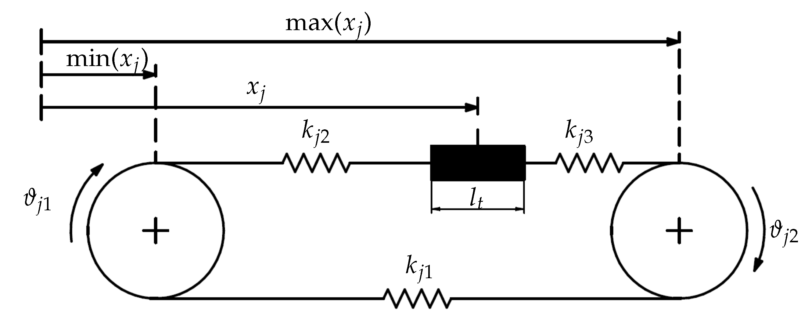
2.3. Belt Transmission Dynamics

As already mentioned, the mass of the belts can be neglected; therefore, the kinetic energy associated to the belt transmission is determined by the rotational inertia not only of the pulleys, but more significantly of the three motors and gearboxes, which are assumed to rotate rigidly with the actuated pulley.

To properly describe the system, six additional coordinates ${\vartheta }_{j,1}$${\vartheta }_{j,2}$ (with $j=1,2,3$) associated to the rotation of the pulleys are required. Figure 6 shows a diagram of the timing belt in which the stiffnesses and the coordinates are highlighted for the $j^{th}$ axis. Which pulley is driven by the motor is shown in Figure 2.

Denoting as $I_{p,j,k}$ the rotational inertia of the pulley described by the coordinate ${\vartheta }_{j,k}$, the kinetic energy of the three transmissions can be expressed in the form

$$\begin{array}{c}\hfill T_t={\displaystyle \frac{1}{2}}\sum _{j=1}^3\left(I_{p,j,1}{\dot{\vartheta }}_{j,1}^2+I_{p,j,2}{\dot{\vartheta }}_{j,2}^2\right),\end{array}$$

(28)

By introducing the array of pulley coordinates

$$\begin{array}{c}\hfill {\mathit{\vartheta }}^{\top }=\left[\begin{array}{cccccc}{\vartheta }_{1,1}& {\vartheta }_{2,1}& {\vartheta }_{3,1}& {\vartheta }_{1,2}& {\vartheta }_{2,2}& {\vartheta }_{3,2}\end{array}\right]\end{array}$$

(29)

and by suitably collecting the mass terms, the kinetic energy of the transmissions can be expressed in matrix notation as

$$\begin{array}{c}\hfill T_t={\displaystyle \frac{1}{2}}{\dot{\mathit{\vartheta }}}^{\top }{\mathit{M}}_{\mathit{t}}\dot{\mathit{\vartheta }}.\end{array}$$

(30)

In Equation (30) the transmission mass matrix ${\mathit{M}}_{\mathit{t}}$ is a 6-by-6 diagonal and constant matrix. For the subsequent analyses, pulleys having the following characteristics are considered:

• Radius $R_p=35$ mm,
• Inertia around the rotation axis $I_{p,j}=130 \times {10}^{-6}$ kg · m².

Furthermore, the motor and gearbox inertia—suitably projected on the machine side through the gearbox reduction rate—is added to the inertia of the actuated pulleys.

3. Overall Dynamics

The total kinetic energy of the system can then be expressed as:

$$\begin{array}{c}\hfill T(\mathit{x},\mathit{\vartheta },\dot{\mathit{x}},\dot{\mathit{\vartheta }})=T_{ss}(\mathit{x},\dot{\mathit{x}})+T_t(\mathit{\vartheta },\dot{\mathit{\vartheta }}).\end{array}$$

(31)

Introducing the array of the free coordinates of the overall system as

$$\begin{array}{c}\hfill \mathit{q}=\left[\begin{array}{c}\mathit{x}\\ \mathit{\vartheta }\end{array}\right],\end{array}$$

(32)

the complete mass matrix can be easily assembled:

$$\begin{array}{c}\hfill \mathit{M}=\left[\begin{array}{cc}{\mathit{M}}_{\mathit{ss}}& \mathbf{0}\\ \mathbf{0}& {\mathit{M}}_{\mathit{t}}\end{array}\right].\end{array}$$

(33)

The overall mass matrix is a function of the trucks’ positions. In a similar way, the mechanical stiffness of each transmission changes with the position of the truck, as this defines the free lengths of the three segments of which the timing belt is composed. As already highlighted in Section 2.1, the specific stiffness $k_{sp}$ quantifies the stiffness of the timing belt for each unit length and unit width of the belt itself, and as such, it is one of the parameters commonly specified within the product datasheet. For a given configuration, the stiffness coefficients of the belt sections are therefore computed according to the following equation:

$$\begin{array}{c}\hfill k_{j,k}={\displaystyle \frac{w_b{k}_{sp}}{l_{f,j,k}}},\end{array}$$

(34)

in which $w_b$ is the belt width, and $l_{f,j,k}$ is the free length of the considered belt segment.

More explicitly, the stiffness coefficients for each belt transmission are computed as

$$\begin{array}{ccc}& k_{j,1}=& w_b{k}_{sp}{\left(max\left(x_j\right)-min\left(x_j\right)\right)}^{-1}\hfill \end{array}$$

(35)

$$\begin{array}{ccc}& k_{j,2}=& w_b{k}_{sp}{\left(x_j^{*}-min\left(x_j\right)-{\displaystyle \frac{1}{2}}{l}_t\right)}^{-1}\hfill \end{array}$$

(36)

$$\begin{array}{ccc}& k_{j,3}=& w_b{k}_{sp}{\left(max\left(x_j\right)-x_j^{*}-{\displaystyle \frac{1}{2}}{l}_t\right)}^{-1},\hfill \end{array}$$

(37)

where $x_j^{*}$ represents the undeformed $j^{th}$ truck coordinate, $l_t$ is the length of the truck, and $min\left(x_j\right)$ and $max\left(x_j\right)$, shown in Figure 6, are fixed structural parameters that correspond to the maximum and minimum displacements achievable by an ideally dimensionless cart.

If large rigid motions of the system are considered, the elastic actions do not admit a potential function, due to the non-constant stiffness coefficients. However, if small displacements around a given undeformed configuration are to be investigated, the stiffness variations can be neglected, and an elastic potential for each belt can be determined as

$$\begin{array}{c}\hfill U_{el,j}=-{\displaystyle \frac{1}{2}}\left(k_{j,1}{\left(R_p\left(\Delta {\vartheta }_{j,2}-\Delta {\vartheta }_{j,1}\right)\right)}^2+k_{j,2}{\left(\Delta x_j-R_p\Delta {\vartheta }_{j,2}\right)}^2+k_{j,3}{\left(R_p\Delta {\vartheta }_{j,1}-\Delta x_j\right)}^2\right).\end{array}$$

(38)

Here, the variables $\Delta {\vartheta }_{j,1}$, $\Delta {\vartheta }_{j,2}$ and $\Delta x_j$ are to be interpreted as displacements around the undeformed configuration ${\vartheta }_{j,1}^{*}$, ${\vartheta }_{j,2}^{*}$, $x_j^{*}$:

$$\begin{array}{c}\hfill \Delta {\vartheta }_{j,1}={\vartheta }_{j,1}-{\vartheta }_{j,1}^{*}\end{array}$$

(39)

$$\begin{array}{c}\hfill \Delta {\vartheta }_{j,2}={\vartheta }_{j,2}-{\vartheta }_{j,2}^{*}\end{array}$$

(40)

$$\begin{array}{c}\hfill \Delta x_j=x_j-x_j^{*}.\end{array}$$

(41)

The potential function of the free system can then be obtained by summation of the gravitational and elastic potentials:

$$\begin{array}{c}\hfill U\left(\mathit{q}\right)=U_g\left(\mathit{x}\right)+\sum _{j=1}^3{U}_{el,j}\left(\mathit{q}\right).\end{array}$$

(42)

The dynamic model describes a semi-definite system, which therefore can undergo rigid motions. Indeed, the motors apply torques to the system and do not set the position of the actuated pulleys. The equilibrium condition of the system, for a given position of the end-effector, can, however, be evaluated by introducing static torques ${\tau }_{st,1}$, ${\tau }_{st,2}$, ${\tau }_{st,3}$ applied to the actuated pulleys in order to keep the end-effector in the desired configuration.

The external generalized forces acting on the generalized coordinates of the system can therefore be expressed in vector notation as

$$\begin{array}{c}\hfill \mathit{Q}={\left[\begin{array}{ccccccccc}0& 0& 0& {\tau }_{st,1}& 0& 0& 0& {\tau }_{st,2}& {\tau }_{st,3}\end{array}\right]}^{\top }.\end{array}$$

(43)

It should be noted that the vector $\mathit{Q}$ defined in (43) is consistent with the location of the motors reported in Figure 2, and thus properly distinguishes the actuated degrees of freedom (namely ${\vartheta }_{1,1}$, ${\vartheta }_{2,2}$ and ${\vartheta }_{3,2}$) from the passive ones. In more detail, the position of the static torques within vector $\mathit{Q}$ corresponds to the position of the driven pulleys’ rotational angles in vector $\mathit{q}$. The other elements of vector $\mathit{Q}$ are equal to zero because they correspond to the position of the non-actuated coordinates.

A static equilibrium configuration should satisfy the condition

$$\begin{array}{c}\hfill \nabla U\left(\mathit{q}\right)+\mathit{Q}=0.\end{array}$$

(44)

The solution of the set of Equation (44) yields the static equilibrium configuration around which we develop the modal analysis. In particular, the static torques and the pulleys’ rotations are the unknowns of the problem, while the displacements of the trucks, which alone define the position of the mobile platform, are fixed. This choice is motivated by the need to express the several results of the modal analysis as functions of the mobile platform coordinates, as this can shed additional insight also on the functional characteristics of the robotic device.

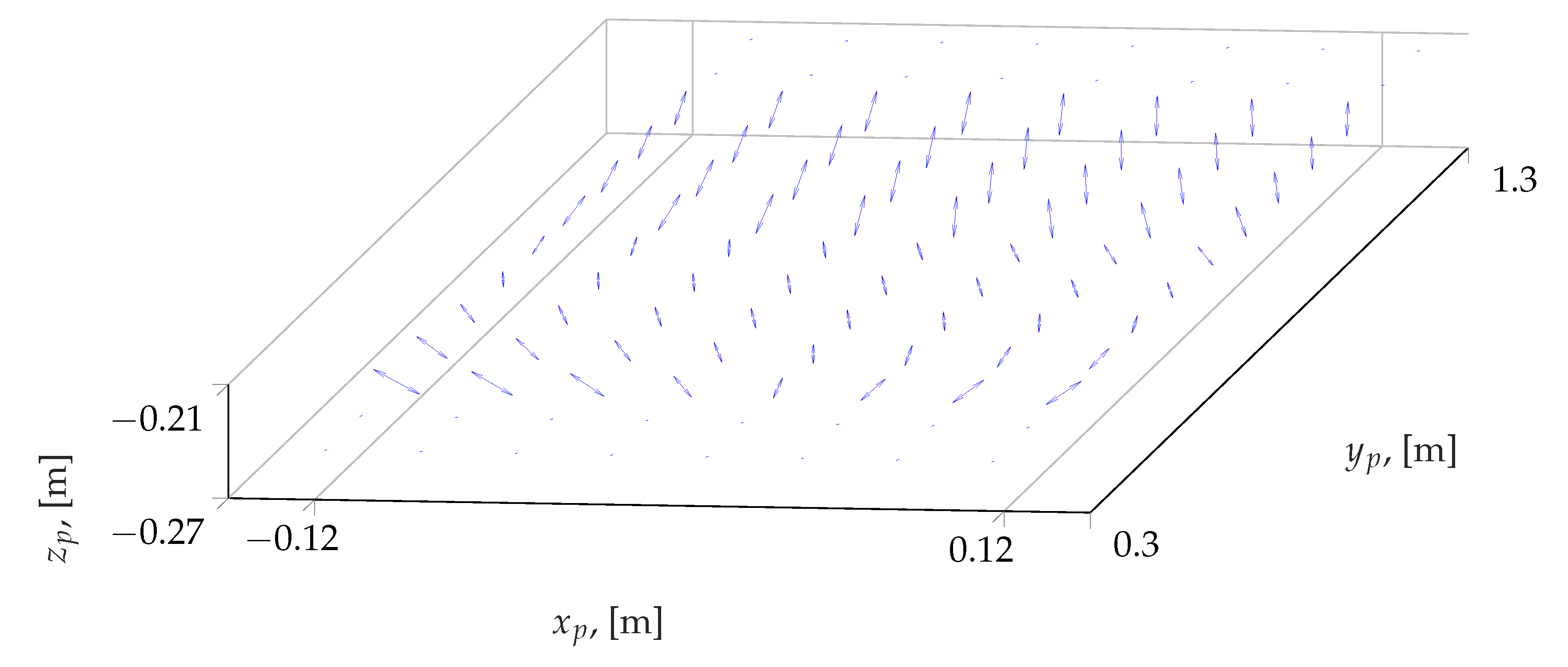
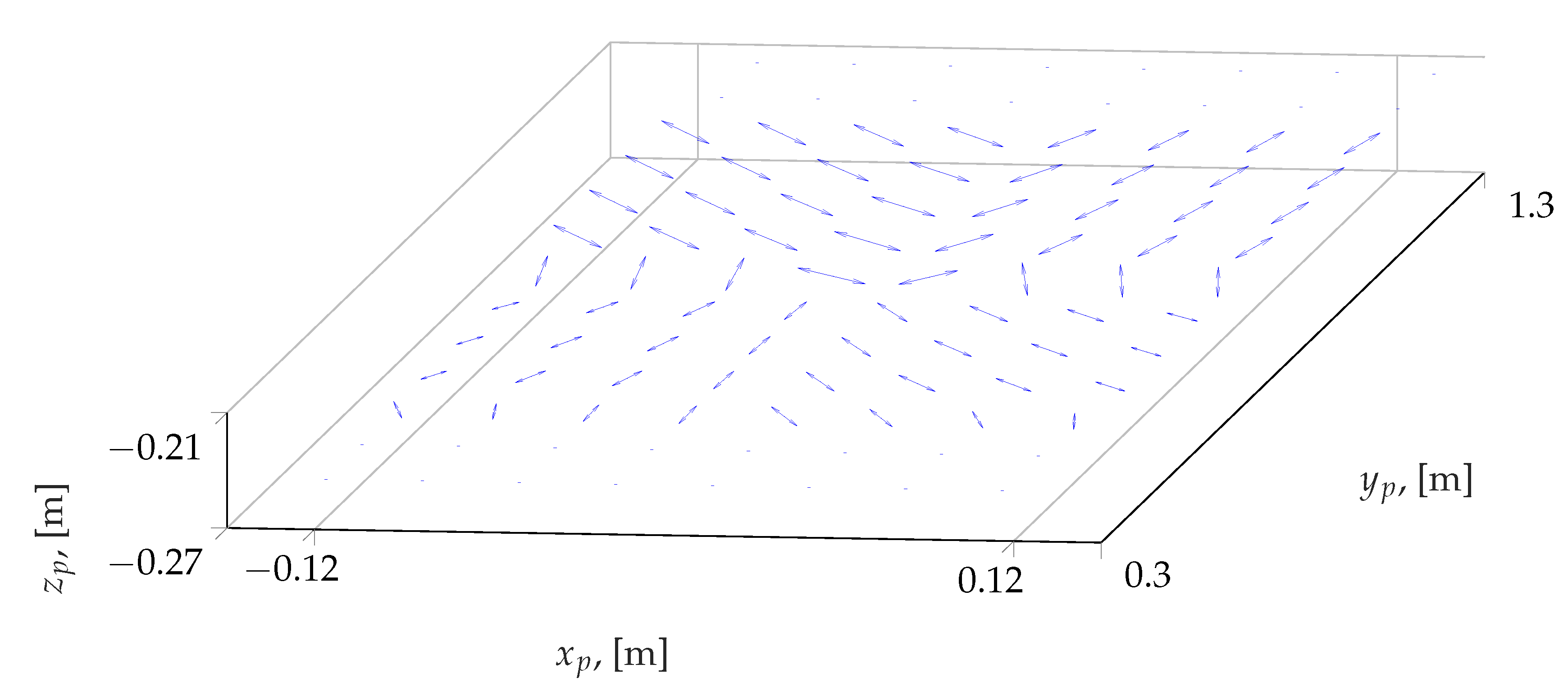
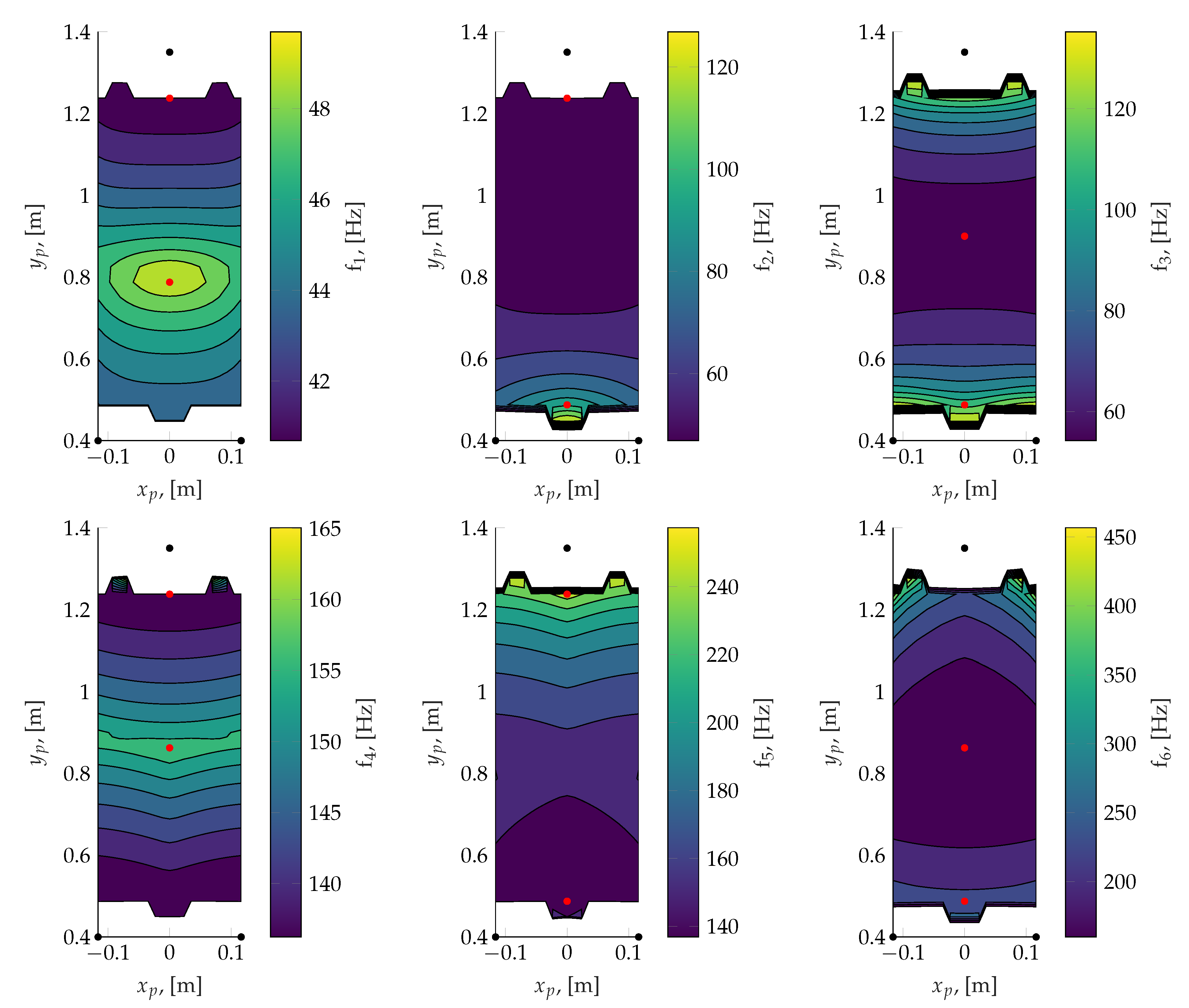
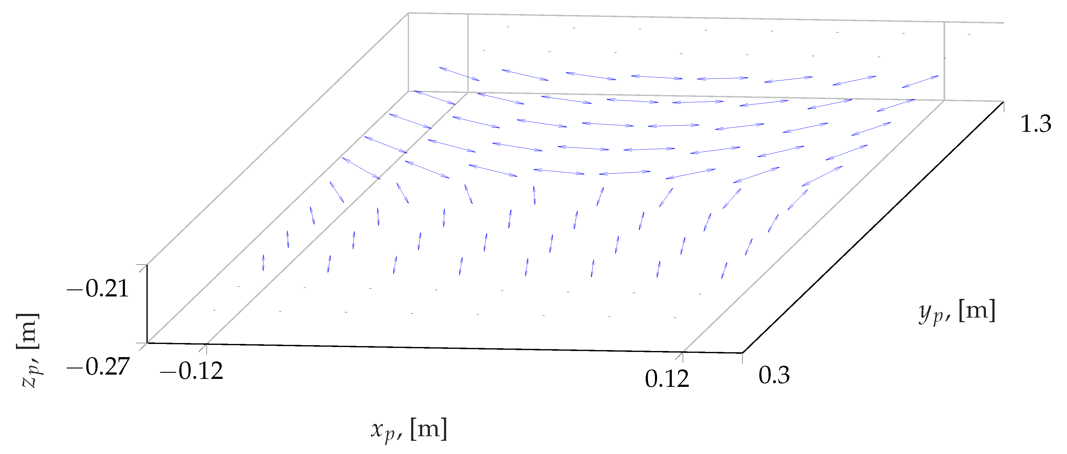
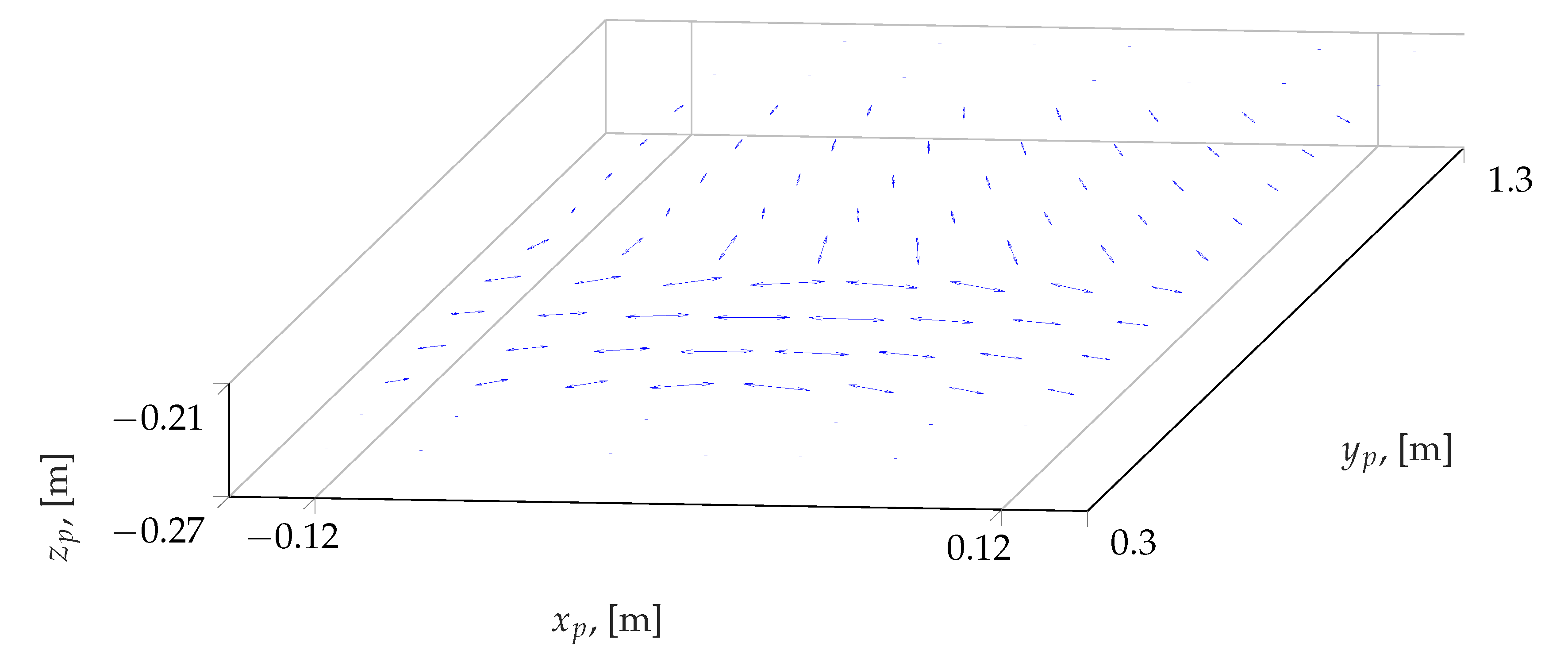
4. Configuration-Dependent Modal Analysis

The modal analysis around a given equilibrium configuration ${\mathit{q}}_{eq}$ can be performed by substituting into Lagrange’s equations the approximated kinetic energy and potential functions.

In particular,

$$\begin{array}{ccc}\hfill \tilde{T}\left(\dot{\mathit{q}}\right)& =& T({\mathit{q}}_{eq},\dot{\mathit{q}})\hfill \end{array}$$

(45)

$$\begin{array}{ccc}\hfill \tilde{U}\left(\mathit{q}\right)& =& U\left({\mathit{q}}_{eq}\right)+\nabla U\left({\mathit{q}}_{eq}\right)(\mathit{q}-{\mathit{q}}_{eq})+{\displaystyle \frac{1}{2}}{(\mathit{q}-{\mathit{q}}_{eq})}^{\top }{\mathit{H}}_{\mathit{U}}\left({\mathit{q}}_{eq}\right)(\mathit{q}-{\mathit{q}}_{eq}),\hfill \end{array}$$

(46)

where ${\mathit{H}}_{\mathit{U}}$ is the Hessian matrix of the total potential.

Lagrange’s equations assume the form

$$\begin{array}{c}\hfill {\displaystyle \frac{d}{dt}}{\displaystyle \frac{\partial \tilde{T}}{\partial \dot{\mathit{q}}}}-{\displaystyle \frac{\partial \tilde{U}}{\partial \mathit{q}}}=\mathit{Q}.\end{array}$$

(47)

Remembering the equilibrium conditions, Equation (47) can be written in the familiar matrix notation,

$$\begin{array}{c}\hfill \mathit{M}\ddot{\mathit{q}}+\mathit{K}\mathit{q}=0,\end{array}$$

(48)

in which the stiffness matrix is simply defined as $\mathit{K}=-{\mathit{H}}_{\mathit{U}}$.

It might be observed that the Hessian matrix associated to $U_{el,}$ can be analytically obtained by double differentiation, while the one relative to the gravitational potential $U_g$ is computed using the following property of the time derivative of the Jacobian matrices—chiefly ${\mathit{D}}_{\mathit{p}}$—that govern the gradient $\nabla U_g$,

$$\begin{array}{c}\hfill {\dot{\mathit{D}}}_{\mathit{p}}(\mathit{x},\dot{\mathit{x}})=\sum _{j=1}^3{\displaystyle \frac{\partial }{\partial x_j}}{\mathit{D}}_{\mathit{p}}{\dot{x}}_j.\end{array}$$

(49)

Evaluating ${\dot{\mathit{D}}}_{\mathit{p}}(\mathit{x},{\delta }_{\mathit{jk}})$, with ${\delta }_{\mathit{jk}}$ being Kronecker’s Delta, the partial derivatives ${\displaystyle \frac{\partial }{\partial x_j}}{\mathit{D}}_{\mathit{p}}$ can be recovered, from which, in turn, the Hessian matrix of the gravitational potential can be straightforwardly constructed.

The mass and stiffness matrices are constant for each position ${\mathit{q}}_{eq}$, taken into account inside the investigated workspace. For each position, an eigenvalue problem for the matrix ${\mathit{M}}^{-1}\mathit{K}$ is then set up and solved in order to highlight the configuration-dependent natural frequencies and modal vectors of the system. As expected, the first three modes represent the rigid motions of the system, while the remaining six are proper vibration modes.

Although a detailed workspace analysis of the manipulator is outside the scope of this work, the investigation refers to a significant working plane selected by the Jacobian’s condition number of the rigid subsystem. The Jacobian’s condition number of the chosen plane is more uniformly distributed and has the lower mean value, i.e., 3.5. Figure 7 shows the selected plane at the position $z=-245$. An equally distributed sampling of this plane defines the investigated end-effector’s pose, giving the equilibrium positions ${\mathit{q}}_{eq}$.

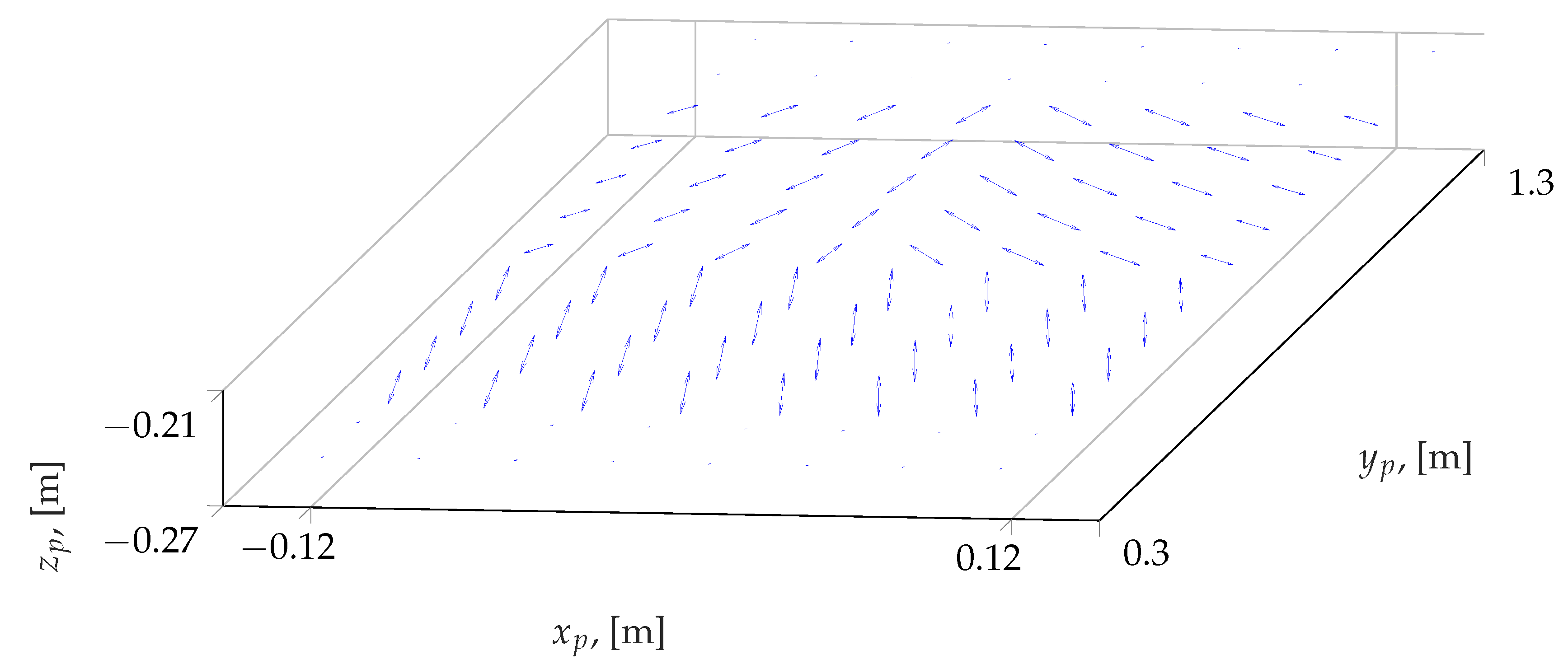
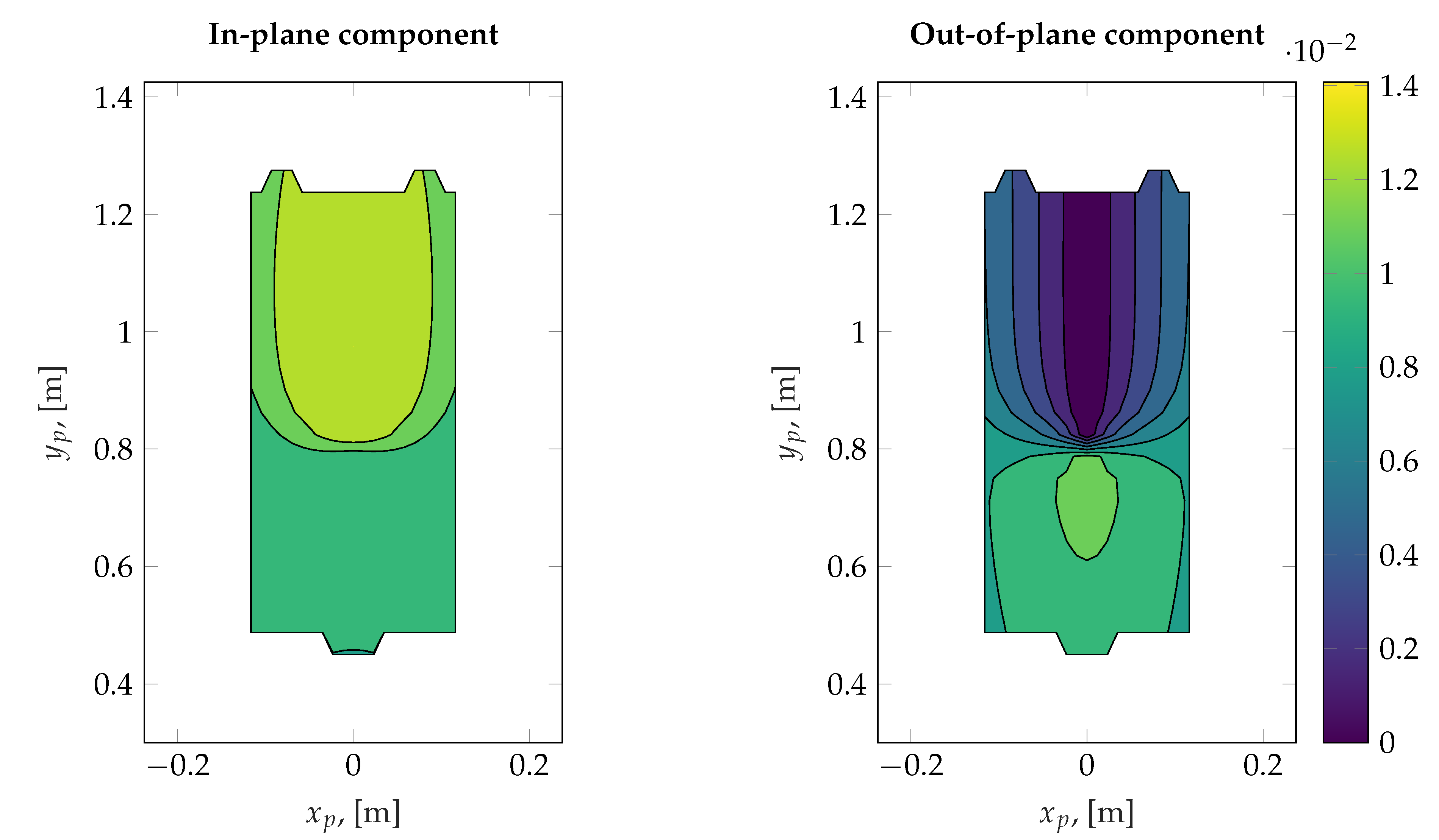
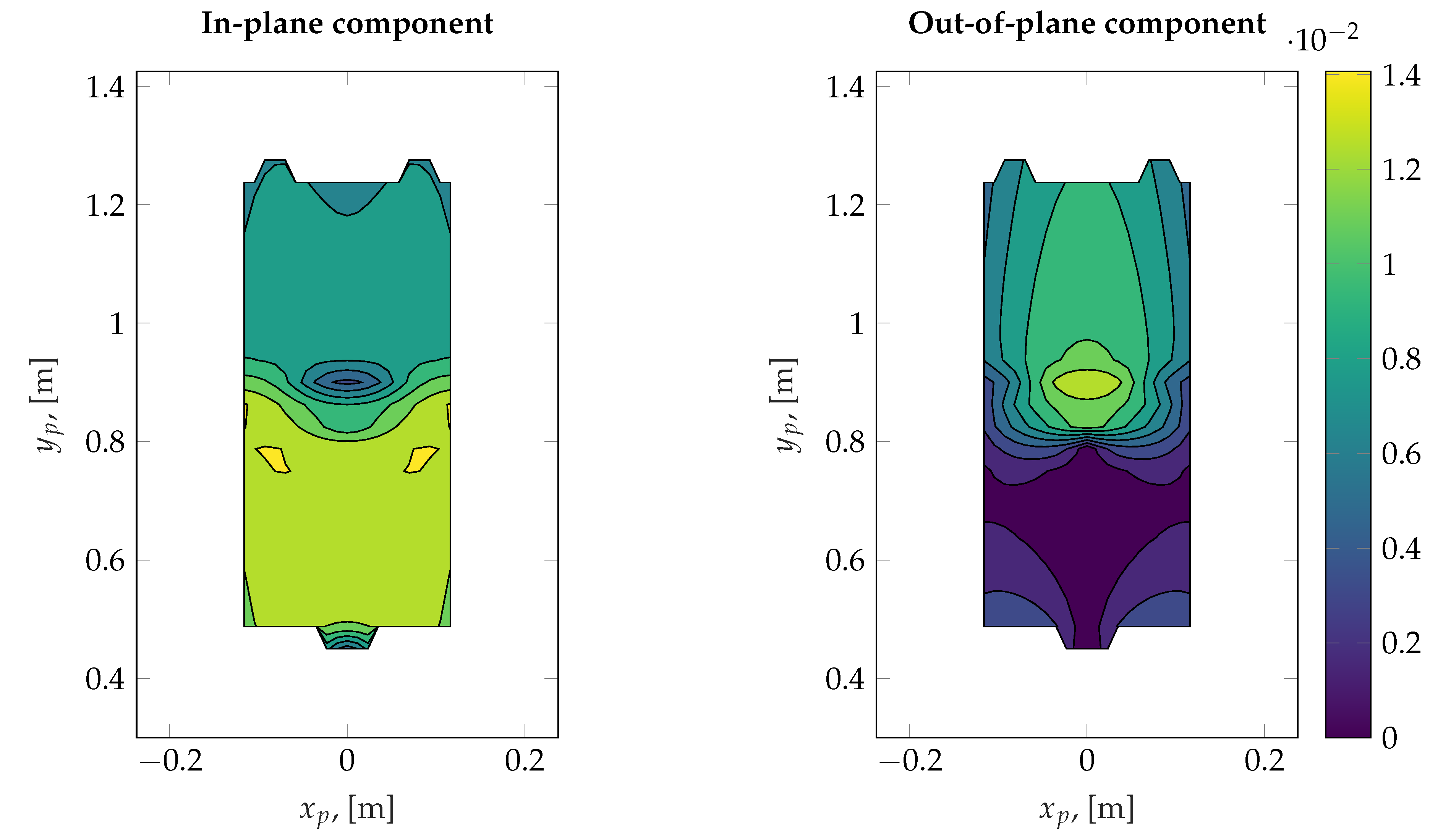
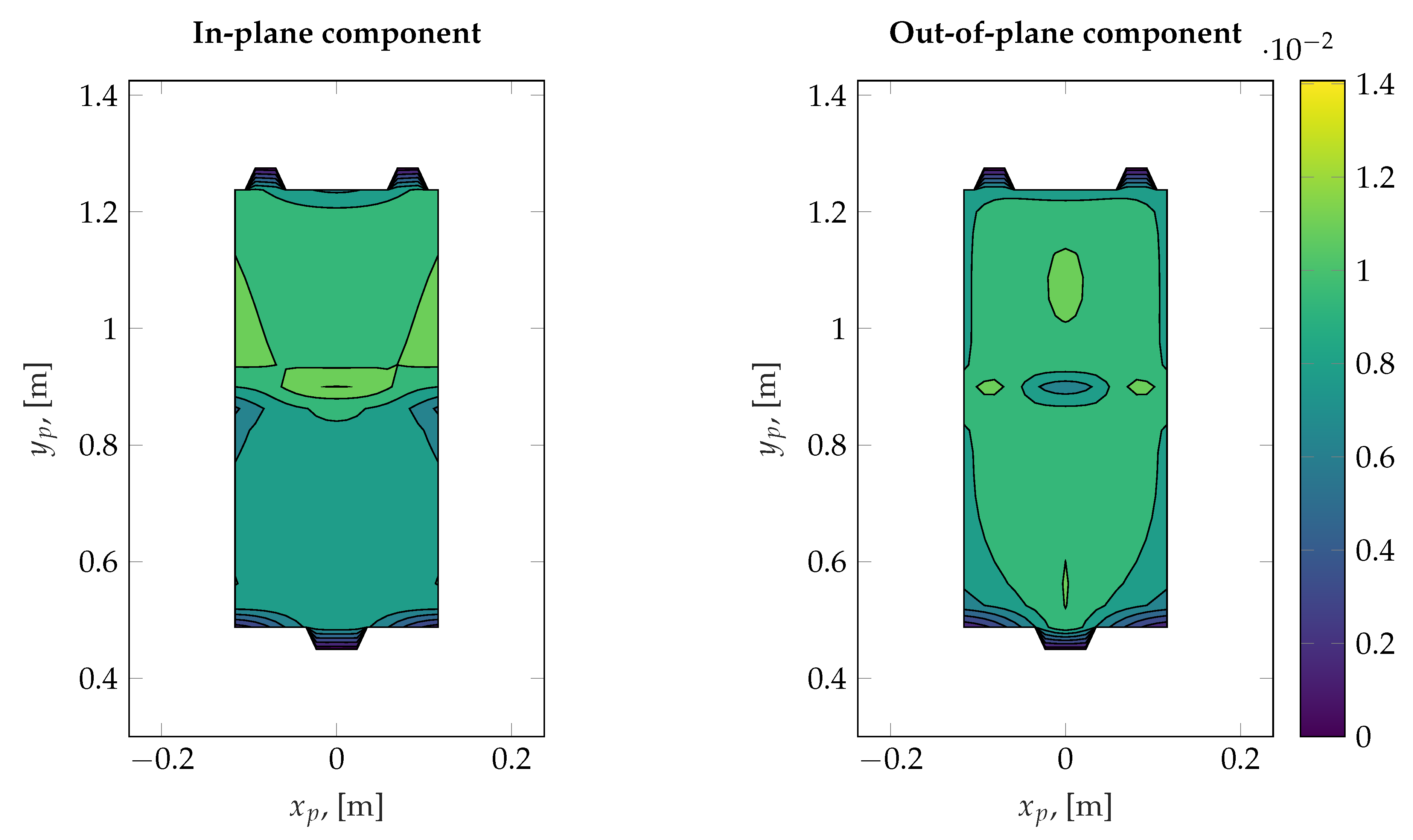
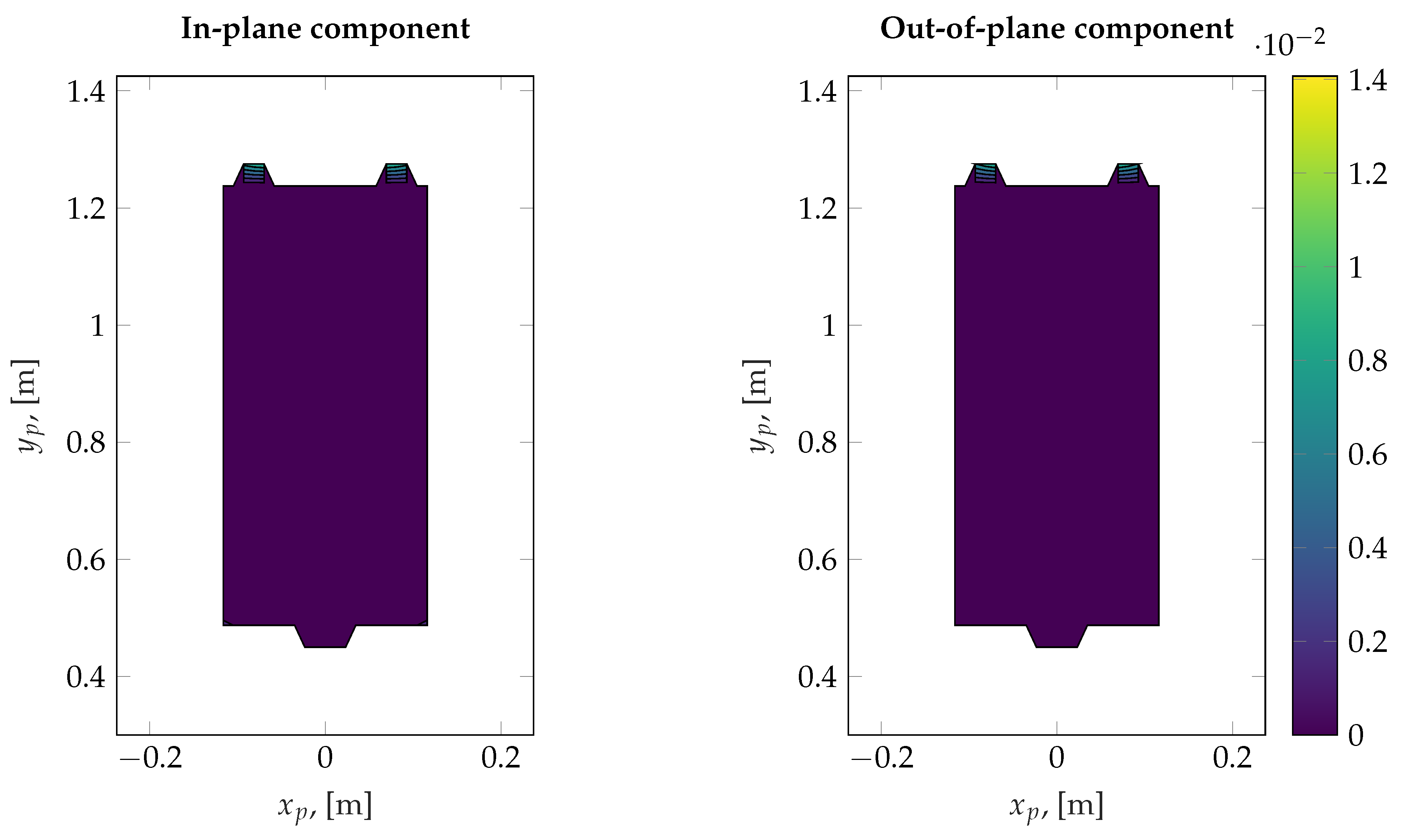
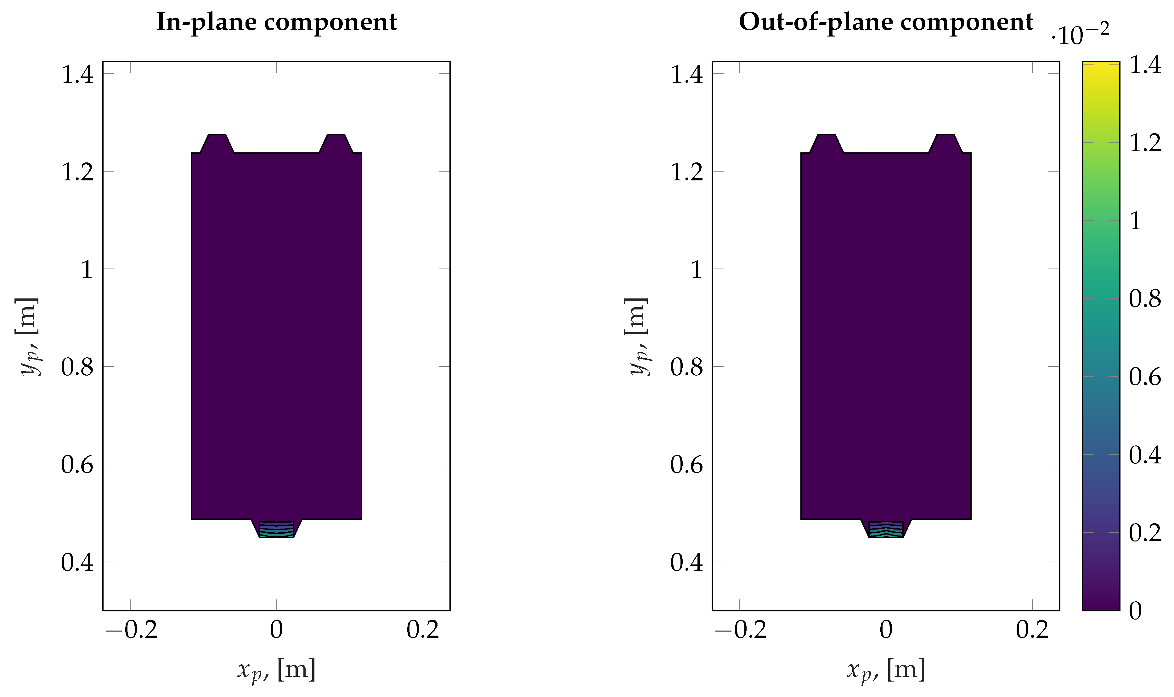
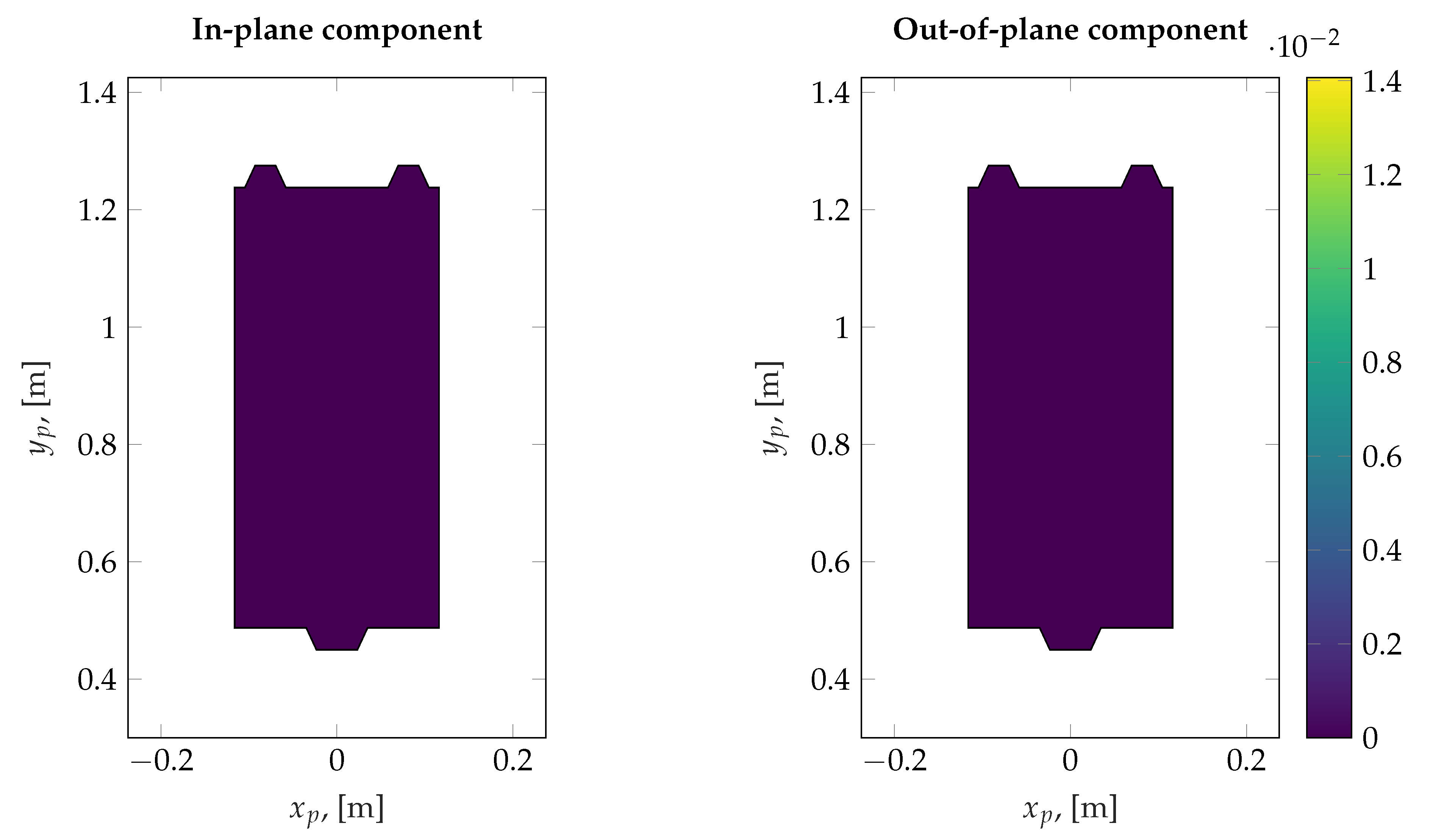
5. Results and Discussion

This section presents the results of the modal analysis developed on the end-effector’s positions belonging to the plane defined in the previous section. The software package selected for the implementation of the system’s model, and for the development of the modal analysis for different end-effector’s positions is MathWorks^® Matlab^®, owing to its matrix processing and data visualization capabilities. The first results reported are the natural frequencies for each of the six modes of vibration (the remaining three, related to the rigid motion of the system, are not included); $f_1-f_6$ are the natural frequencies (expressed in Hz) of the modes 1 to 6, sorted in ascending order. In particular, Figure 8 shows how the natural frequencies change by changing the position($x_p$, $y_p$) of the end-effector on the reference plane. The red markers are positioned along a line corresponding to the direction of the central axis (axis 1) at points, within the useful working area (boundary effects excluded), where the natural frequencies have their maximum and minimum value. The black markers qualitatively indicate the position of the three motors.

As expected, all the graphs are symmetric with respect to the system’s central linear axis (axis 1), while the change of the natural frequencies along the y axis depends on the specific mode of vibration. Regarding the first mode, the graph shows that the frequency has its maximum value located in the lower half of the reference plane; starting from this point, moving toward the upper or the lower end of the working plane (i.e., increasing of decreasing coordinate $y_p$), the frequency decreases, reaching its minimum value at the upper end. For the second mode, minimum and maximum values correspond, respectively, to the upper end and to the lower end of the working area. Moving toward lower $y_p$ coordinate values, the frequency increases with a gradient more significant in the lower half of the area. The third mode has the frequency’s minimum value at approximately the middle of the working area, and the frequency increases, both increasing and decreasing coordinate $y_p$. The gradient of the frequency becomes quite significant near the ends of the area. For the fourth mode, the behavior is almost symmetric also along the y direction, with the maximum value at the upper end and the minimum value in the middle. The fifth mode is characterized by a progressive increase of the frequency from the lower end to the higher one. The sixth mode has the minimum value located approximately in the middle of the area, and the maximum value at the lower end. Again, the frequency increases, both increasing and decreasing the position $y_p$, but with a gradient higher in the upper half rather than in the lower one.

However, the information concerning the natural frequencies is not enough to completely understand the system’s behavior. As a matter of fact, even if we know the frequency of vibration corresponding to a specific mode, we do not know how the system vibrates according to the mode. So we do not know which is the influence of that specific mode on the behavior of the end-effector. In order to reach this goal, the attention must be focused on the modal vectors and on their projection on the end-effector’s coordinates; this is the key point. The values of the modal vectors for the positions corresponding to the minimum and maximum values of the frequency, taken along the symmetry axis of the plane within the workspace area not affected by boundary effects, are summarized for each mode of vibration in

Table 1. Modal vector for each natural frequency, at the point of minimum.

Mode	$\mathit{f},\left[\mathit{Hz}\right]$	${\mathit{x}}_1/{\mathit{R}}_{\mathit{p}}$	${\mathit{x}}_2/{\mathit{R}}_{\mathit{p}}$	${\mathit{x}}_3/{\mathit{R}}_{\mathit{p}}$	${\mathit{\vartheta }}_{1,1}$	${\mathit{\vartheta }}_{2,1}$	${\mathit{\vartheta }}_{3,1}$	${\mathit{\vartheta }}_{1,2}$	${\mathit{\vartheta }}_{2,2}$	${\mathit{\vartheta }}_{3,2}$
1	40.873	−6.77 × 10${}^{-15}$	−3.19 × 10${}^{-1}$	3.19 × 10${}^{-1}$	−9.69 × 10${}^{-15}$	−1.37 × 10${}^{-1}$	1.37 × 10${}^{-1}$	−8.31 × 10${}^{-15}$	1.00	−1.00
2	46.854	−4.04 × 10${}^{-4}$	−2.54 × 10${}^{-2}$	−2.54 × 10${}^{-2}$	−1.50 × 10${}^{-2}$	−5.02 × 10${}^{-1}$	−5.02 × 10${}^{-1}$	−1.50 × 10${}^{-2}$	1.00	1.00
3	54.286	−1.89 × 10${}^{-2}$	−6.88 × 10${}^{-3}$	−6.88 × 10${}^{-3}$	1.00	−5.35 × 10${}^{-2}$	−5.35 × 10${}^{-2}$	3.94 × 10${}^{-2}$	2.50 × 10${}^{-1}$	2.50 × 10${}^{-1}$
4	136.237	−4.90 × 10${}^{-5}$	−9.67 × 10${}^{-7}$	−9.67 × 10${}^{-7}$	7.36 × 10${}^{-2}$	−3.35 × 10${}^{-5}$	−3.35 × 10${}^{-5}$	−1.00	2.37 × 10${}^{-6}$	2.37 × 10${}^{-6}$
5	136.835	2.17 × 10${}^{-5}$	7.78 × 10${}^{-4}$	7.78 × 10${}^{-4}$	−5.46 × 10${}^{-5}$	−1.00	−1.00	7.79 × 10${}^{-4}$	4.15 × 10${}^{-2}$	4.15 × 10${}^{-2}$
6	159.823	−5.25 × 10${}^{-5}$	−1.23 × 10${}^{-3}$	−1.23 × 10${}^{-3}$	−4.13 × 10${}^{-4}$	1.00	1.00	1.92 × 10${}^{-2}$	−2.40 × 10${}^{-2}$	−2.40 × 10${}^{-2}$

and

Table 2. Modal vector for each natural frequency, at the point of maximum.

Mode	$\mathit{f},\left[\mathit{Hz}\right]$	${\mathit{x}}_1/{\mathit{R}}_{\mathit{p}}$	${\mathit{x}}_2/{\mathit{R}}_{\mathit{p}}$	${\mathit{x}}_3/{\mathit{R}}_{\mathit{p}}$	${\mathit{\vartheta }}_{1,1}$	${\mathit{\vartheta }}_{2,1}$	${\mathit{\vartheta }}_{3,1}$	${\mathit{\vartheta }}_{1,2}$	${\mathit{\vartheta }}_{2,2}$	${\mathit{\vartheta }}_{3,2}$
1	49.692	5.33 × 10${}^{-1}$	−5.35 × 10${}^{-3}$	−5.35 × 10${}^{-3}$	−1.00	5.05 × 10${}^{-3}$	5.05 × 10${}^{-3}$	3.63 × 10${}^{-2}$	2.06 × 10${}^{-2}$	2.06 × 10${}^{-2}$
2	126.906	−2.14 × 10${}^{-17}$	1.17 × 10${}^{-2}$	−1.17 × 10${}^{-2}$	1.45 × 10${}^{-16}$	−6.46 × 10${}^{-1}$	6.46 × 10${}^{-1}$	−6.19 × 10${}^{-16}$	−1.00	1.00
3	135.238	−7.71 × 10${}^{-4}$	−2.68 × 10${}^{-2}$	−2.68 × 10${}^{-2}$	2.68 × 10${}^{-3}$	2.65 × 10${}^{-1}$	2.65 × 10${}^{-1}$	−2.37 × 10${}^{-2}$	1.00	1.00
4	157.310	8.51 × 10${}^{-4}$	5.57 × 10${}^{-6}$	5.57 × 10${}^{-6}$	2.55 × 10${}^{-2}$	9.86 × 10${}^{-3}$	9.86 × 10${}^{-3}$	−1.00	−2.75 × 10${}^{-4}$	−2.75 × 10${}^{-4}$
5	250.799	4.92 × 10${}^{-19}$	6.90 × 10${}^{-4}$	−6.90 × 10${}^{-4}$	−3.36 × 10${}^{-16}$	−1.00	1.00	−2.27 × 10${}^{-17}$	9.76 × 10${}^{-3}$	−9.76 × 10${}^{-3}$
6	263.843	1.16 × 10${}^{-3}$	2.78 × 10${}^{-5}$	2.78 × 10${}^{-5}$	8.66 × 10${}^{-3}$	−1.10 × 10${}^{-4}$	−1.10 × 10${}^{-4}$	−1.00	−1.74 × 10${}^{-4}$	−1.74 × 10${}^{-4}$

. The truck translations are divided by the pulley radius to compare non-homogeneous linear and angular coordinates fairly.

In both Table 1 and Table 2, it can be seen that the motion of the free pulley is dominant within the modal vectors of modes 4, 5, and 6; on the other hand, the component associated to the actuated pulleys is the most significant for modes 1, 2 and 3. This rather clean distinction between lower and higher frequency modes is also reflected in the magnitude of the displacements of the trucks; indeed the maximum absolute truck displacement over modes 1, 2 and 3 is at least one order of magnitude greater than that of modes 4, 5 and 6.

The kinematic modal analysis results are also represented from the working space point of view, highlighting, for different positions on the reference plane, the directions of the end-effector’s displacement as a consequence of the projection of the modal vector components related to the carriages’ displacement. In other words, they represent the projection of the modal vectors after suitable normalization on the mobile platform using the Jacobian matrix ${\mathit{D}}_{\mathit{p}}$. The direction of the end-effector’s displacements are represented, for modes 1 to 6, in Figure 9, Figure 10, Figure 11, Figure 12, Figure 13 and Figure 14.

From the analysis of these diagrams, it is evident that the direction of vibration of the end-effector, due to a specific mode of vibration, strongly depends on its position within the reference plane. For all the modes, the displacement directions are symmetric with respect to the central axis, and they progressively change by changing the $y_p$ coordinate. Figure 15, Figure 16, Figure 17, Figure 18, Figure 19 and Figure 20 represent, in another way, the same modal vectors, focusing on values of in-plane and out-of-plane displacements rather than on the directions of vibration, using the same modal vector normalization for all the figures.

The figures on the left represent the displacement in the $x-y$ plane, while the figures on the right represent the displacement in the z direction.

This approach highlights the first-order effects of the truck displacements on the displacement of the end-effector. The in-plane component was defined and represented as $\sqrt{\delta p_1^2+\delta p_2^2}$, where $\delta p_1$ and $\delta p_2$ are the first two components of the modal vector projected on the end-effector, while the absolute value of the vertical out of plane component $\delta p_3$ is represented separately. The vibrational displacements of the mobile platform are represented using the same scale, allowing a quantitative comparison between the effects of different modes.

In particular, Figure 15, Figure 16 and Figure 17 are related to the first three modes and show that, for these modes, the direction’s displacements of the end-effector, both along the reference plane and along the vertical direction, are significant (please note that the color bars of the graphs have all the same scale). Moreover, the shape of the diagrams is clearly symmetric with respect to the central axis. As far as the y direction is concerned, Figure 15, which refers to the first mode of vibration, shows that the upper half of the working plane, the one nearer to motors 1 and 2, is characterized by values of in-plane displacements lower than the ones corresponding to the lower half-plane, the one nearer to motor 1. Hence, displacements increase as the $y_p$ coordinate increases. For the out-of-plane components graph, the behavior is opposite: as $y_p$ coordinate increases, the displacement decreases. The displacement’s maximum value is located in a small area just below the half of the plane. Moreover, it should be noted that along the symmetry axis, there is a position near to the middle of the area where the vertical displacement has a sudden change.

As regards the second mode of vibration, Figure 16 shows an opposite behavior with respect to Figure 15, for both the in-plane and out-of-plane displacements. The in-plane displacement decreases as the $y_p$ coordinate increases, with the minimum value located just above the central position, and the maximum one located in small areas on opposite sides just below the center of the plane. On the contrary, the vertical displacement increases as the $y_p$ coordinate increases, and there is an area around the middle of the plane where it has its maximum value and where a sudden change occurs.

For the in-plane displacement related to the third mode of vibration (Figure 17), the working plane is again divided in two equal parts: the lower one is characterized by values lower than the upper part. Moreover, no sudden changes are highlighted, just small areas where the values slightly change with respect to the values of the respective half area. The out-of-plane component is quite uniformly distributed along the plane, with a central area where the values increase and some areas are located approximately near the ends of the plane’s horizontal and vertical middle lines where the values decrease.

As regards the displacements related to the fourth, fifth and sixth modes, respectively depicted in Figure 18, Figure 19 and Figure 20, the displacements, both in-plane and out-of-plane, of the end-effector are clearly negligible. This confirms on the entire working plane that—as already seen for some notable configurations analyzed in Table 1 and Table 2—the truck displacements associated to modes 4, 5 and 6 are comparatively smaller, and thus do not generate appreciable motions at the end-effector.

6. Conclusions

The proposed approach is applied to a parallel kinematic manipulator with driven joints characterized by low mechanical stiffness. It outlines the effects of the stiffness of the transmission, of the mass distribution and of the coupling between the joints due to the parallel kinematic chains on the end-effector’s vibration direction and magnitude. The mathematical approach considers the masses of all the elements of the parallel kinematic part, the system’s actual configuration, i.e., that it is subject to a motion control algorithm, where the motors are torque controlled, and the transmissions’ stiffness, leading to a 9 d.o.f. system. The direction of vibration of the end-effector, which depends on the dynamic configuration of the system, is represented by the modal vector calculated from the equations of the system’s model, linearized around the investigated points of the workspace.

The discussed results show that the magnitude and direction of the modal displacements at the end-effector, evaluated in suitable points of the working space, are influenced by the configuration-dependent mass distribution and transmission’s stiffness.

The method, applied to a linear delta manipulator, highlights that the effects of the different vibration modes can be effectively compared, considering the amplitude of displacement of the end-effector in the $x-y$ plane or z-direction.

Moreover, the discussion of the results outlines that the displacement’s direction of the end-effector changes along the working area as a function of the kinematic and transmission configuration. For the same vibration mode (i.e., the first), in some zones of the working space, the end-effector is subject to vibration in the vertical direction, while in other zones, the displacement’s direction is predominantly horizontal. In the same way, the frequency associated with the mode varies in the workspace. The proposed approach constitutes a useful support for the system’s design in evaluating the end-effector vibration direction for a given vibration mode, in choosing the working area within the plane, in selecting the proper motion laws, and in synthesizing the control system.

Finally, the proposed approach introduces, in an effective and computationally efficient way, the mass distribution and the coupling effects of the parallel kinematic part as a function of the investigated end-effector positions, thanks to the used mathematical approach. Lastly, our work could open the way toward its implementation in the cases of robots where the stiffness of the parallel kinematic part cannot be neglected.

References

1. Clavel, R. DELTA: A fast robot with parallel geometry. Robotica 1988, 8, 105–109. [Google Scholar]
2. Rey, L.; Clavel, R. The Delta Parallel Robot; Boër, C.R., Molinari-Tosatti, L., Smith, K.S., Eds.; Springer: London, UK, 1999. [Google Scholar]
3. Bourim, M.; Clavel, R. The Linear Delta: Developments and Applications; Springer: Munich, Germany, 2010. [Google Scholar]
4. Merlet, J. Parallel Robots; Kluwer Academic Publishers: Oxford, UK, 2000. [Google Scholar]
5. Parallel Kinematic Machines: Theoretical Aspects and Industrial Requirements; Boër, C.R.; Molinari-Tosatti, L.; Smith, K.S. (Eds.) Springer: Berlin/Heidelberg, Germany, 1999. [Google Scholar]
6. Righettini, P.; Lorenzi, V.; Zappa, B.; Ginammi, A.; Strada, R. Design and optimization of a PKM for micromanipulation. Appl. Mech. Mater. 2015, 799, 1088–1095. [Google Scholar] [CrossRef]
7. Nevaranta, N.; Parkkinen, J.; Lindh, T.; Niemelä, M.; Pyrhönen, O.; Pyrhönen, J. Online Estimation of Linear Tooth Belt Drive System Parameters. IEEE Trans. Ind. Electron. 2015, 62, 7214–7223. [Google Scholar] [CrossRef]
8. Poonia, S.; Singh, A.; Singh, J.; Sharma, S.; Kumar, N. Noise Problem Resolution and Sound Quality Improvement of Valve Timing Belt in 4 Cylinders PFI Gasoline Engine; SAE: Warrendale, PA, USA, 2019. [Google Scholar]
9. Belyaev, A.; Eliseev, V.; Irschik, H.; Oborin, E. Contact of two equal rigid pulleys with a belt modelled as Cosserat nonlinear elastic rod. Acta Mech. 2017, 228, 4425–4434. [Google Scholar] [CrossRef] [Green Version]
10. Oborin, E.; Vetyukov, Y.; Steinbrecher, I. Eulerian description of non-stationary motion of an idealized belt-pulley system with dry friction. Int. J. Solids Struct. 2018, 147, 40–51. [Google Scholar] [CrossRef]
11. Vetyukov, Y.; Oborin, E.; Krommer, M.; Eliseev, V. Transient modelling of flexible belt drive dynamics using the equations of a deformable string with discontinuities. Math. Comput. Model. Dyn. Syst. 2017, 23, 40–54. [Google Scholar] [CrossRef]
12. Long, S.; Wang, W.; Yue, X.; Zhang, C. Dynamic Modeling of the Belt Drive System with an Equivalent Tensioner Model. J. Vib. Eng. Technol. 2021. [Google Scholar] [CrossRef]
13. Long, S.; Zhao, X.; Shangguan, W.B.; Zhu, W. Modeling and validation of dynamic performances of timing belt driving systems. Mech. Syst. Signal Process. 2020, 144, 106910. [Google Scholar] [CrossRef]
14. Zhu, H.; Zhu, W.; Hu, Y.; Wang, X. Periodic Response of a Timing Belt Drive System with an Oval Cogged Pulley and Optimal Design of the Pitch Profile for Vibration Reduction. J. Comput. Nonlinear Dyn. 2018, 13. [Google Scholar] [CrossRef]
15. Passos, S.; Manin, L.; Remond, D.; Sauvage, O.; Rota, L.; Besnier, E. Investigation on the Rotational Dynamics of a Timing Belt Drive including an Oval Driving Pulley. J. Vib. Acoust. 2021, 143, 051014. [Google Scholar] [CrossRef]
16. Zhu, H.; Zhu, W.; Fan, W. Dynamic modeling, simulation and experiment of power transmission belt drives: A systematic review. J. Sound Vib. 2021, 491, 115759. [Google Scholar] [CrossRef]
17. Kulkarni, V.; Chandrashekara, C.; Sethuram, D. Modal Analysis of 3-RRR SPM Model. In Lecture Notes in Mechanical Engineering; Springer: Singapore, 2022; pp. 673–678. [Google Scholar] [CrossRef]
18. La Mura, F.; Giberti, H.; Pirovano, L.; Tarabini, M. Theoretical and experimental modal analysis of a 6 PUS PKM. ICINCO 2019, 2, 276–283. [Google Scholar] [CrossRef]
19. Fiore, E.; Giberti, H. A montecarlo approach to test the modes of vibration of a 6-DoF parallel kinematic simulator. In Shock & Vibration, Aircraft/Aerospace, Energy Harvesting, Acoustics & Optics; Springer: Berlin/Heidelberg, Germany, 2017; pp. 315–323. [Google Scholar] [CrossRef]
20. Palmieri, G.; Martarelli, M.; Palpacelli, M.; Carbonari, L. Configuration-dependent modal analysis of a Cartesian parallel kinematics manipulator: Numerical modeling and experimental validation. Meccanica 2014, 49, 961–972. [Google Scholar] [CrossRef]
21. Ren, J.; Cao, Q. Dynamic modeling and frequency characteristic analysis of a novel 3-pss flexible parallel micro-manipulator. Micromachines 2021, 12, 678. [Google Scholar] [CrossRef] [PubMed]
22. Sayahkarajy, M. Mode shape analysis, modal linearization, and control of an elastic two-link manipulator based on the normal modes. Appl. Math. Model. 2018, 59, 546–570. [Google Scholar] [CrossRef]
23. Yang, C.; Li, Q.; Chen, Q. Natural frequency analysis of parallel manipulators using global independent generalized displacement coordinates. Mech. Mach. Theory 2021, 156, 104145. [Google Scholar] [CrossRef]
24. Dong, C.; Liu, H.; Huang, T.; Chetwynd, D. A screw theory-based semi-analytical approach for elastodynamics of the tricept robot. J. Mech. Robot. 2019, 11, 031005. [Google Scholar] [CrossRef]
25. Wu, L.; Dong, C.; Wang, G.; Liu, H.; Huang, T. An approach to predict lower-order dynamic behaviors of a 5-DOF hybrid robot using a minimum set of generalized coordinates. Robot. Comput. Integr. Manuf. 2021, 67, 102024. [Google Scholar] [CrossRef]
26. Hasegawa, A.; Fujimoto, H.; Takahashi, T. Robot Joint Angle Control Based on Self Resonance Cancellation Using Double Encoders. In Proceedings of the 2017 IEEE International Conference on Advanced Intelligent Mechatronics (AIM), Munich, Germany, 3–7 July 2017; pp. 460–465. [Google Scholar] [CrossRef]
27. Oaki, J.; Chiba, Y. Simple Physically Parameterized Observer for Vibration Suppression Control of SCARA Robot with Elastic Joints. IFAC 2017, 50, 6085–6092. [Google Scholar] [CrossRef]
28. Lee, T.; Choi, J.; Rhim, S. Dynamic analysis and parameter estimation of coupled three-link planar manipulator with flexible belt-drive system. J. Mech. Sci. Technol. 2015, 29, 981–988. [Google Scholar] [CrossRef]
29. Negahbani, N.; Giberti, H.; Fiore, E. Error Analysis and Adaptive-Robust Control of a 6-DoF Parallel Robot with Ball-Screw Drive Actuators. J. Robot. 2016, 2016. [Google Scholar] [CrossRef]
30. Negahbani, N.; Giberti, H.; Ferrari, D. A belt-driven 6-DoF parallel kinematic machine. In Nonlinear Dynamics; Springer: Berlin/Heidelberg, Germany, 2016; Volume 1. [Google Scholar] [CrossRef]
31. MDQUADRO srl | Advanced Mechatronic Solutions. Available online: https://www.mdquadro.com (accessed on 15 November 2021).
32. Righettini, P.; Strada, R.; Zappa, B.; Lorenzi, V. Experimental set-up for the investigation of transmissions effects on the dynamic performances of a linear PKM. Mech. Mach. Sci. 2019, 73, 2511–2520. [Google Scholar] [CrossRef]
Figure 1. Linear delta under analysis.
Robotics 10 00132 g001
Figure 2. Diagram of the linear delta.
Robotics 10 00132 g002
Figure 3. On the left: connection links and joints. On the right: local coordinate systems on the mobile platform.
Robotics 10 00132 g003
Figure 4. Vector loops for the three kinematic chains.
Robotics 10 00132 g004
Figure 5. Euler angle for the definition of generic link j orientation.
Robotics 10 00132 g005
Figure 6. Diagram of the j t h linear belt transmission.
Robotics 10 00132 g006
Figure 7. Reference plane position within the working volume (represented in green).
Robotics 10 00132 g007
Figure 8. Natural frequencies.
Robotics 10 00132 g008
Figure 9. Displacement’s direction of the end-effector for mode 1.
Robotics 10 00132 g009
Figure 10. Displacement’s direction of the end-effector for mode 2.
Robotics 10 00132 g010
Figure 11. Displacement’s direction of the end-effector for mode 3.
Robotics 10 00132 g011
Figure 12. Displacement’s direction of the end-effector for mode 4.
Robotics 10 00132 g012
Figure 13. Displacement’s direction of the end-effector for mode 5.
Robotics 10 00132 g013
Figure 14. Displacement’s direction of the end-effector for mode 6.
Robotics 10 00132 g014
Figure 15. In-plane and out-of-plane components of the first modal vector projected on the mobile platform.
Robotics 10 00132 g015
Figure 16. In-plane and out-of-plane components of the second modal vector projected on the mobile platform.
Robotics 10 00132 g016
Figure 17. In-plane and out-of-plane components of the third modal vector projected on the mobile platform.
Robotics 10 00132 g017
Figure 18. In-plane and out-of-plane components of the fourth modal vector projected on the mobile platform.
Robotics 10 00132 g018
Figure 19. In-plane and out-of-plane components of the fifth modal vector projected on the mobile platform.
Robotics 10 00132 g019
Figure 20. In-plane and out-of-plane components of the sixth modal vector projected on the mobile platform.
Robotics 10 00132 g020