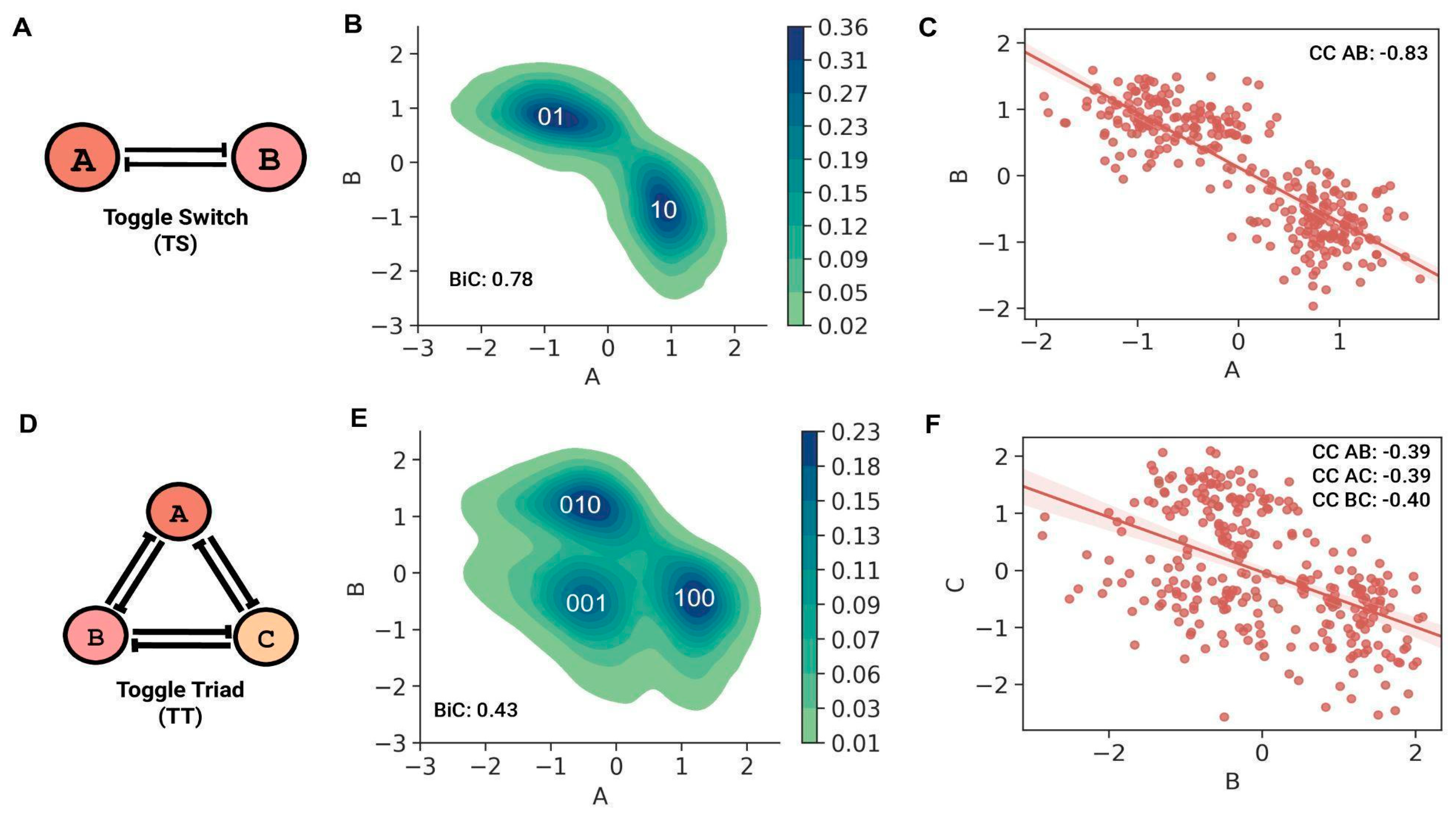
3.1. Stand-Alone Properties of Toggle Switch and Toggle Triad
We first investigated the stand-alone properties of a toggle TS and TT before embedding them in larger networks. RACIPE formalism [
23] (see
Section 2) was used to simulate these networks for 10,000 randomized parameter sets sampled from a predetermined parameter space. Three such replicates (each with 10,000 parameter sets × 100 initial conditions per parameter set) were performed for each motif. The resultant steady-state values for each node were normalized and converted to Z-scores. Pairwise correlation coefficients (CC) were then calculated between the steady state values of nodes in a TS or TT. Furthermore, for the TS, we calculated Sarle’s bimodality coefficient (BiC) [
24] values for each node. BiC values range from 0 to 1, with values closer to 1 representing higher bimodality, and any value above 0.55 is considered to represent a bimodal distribution [
24].
The TS motif (
Figure 1A) mainly showed two “single-positive” steady states: ((low A, high B); (A, B) = (0, 1)) and ((high A, low B); (A, B) = (1, 0)), as observed in the bivariate plot (
Figure 1B). The steady-state values of both nodes in a TS showed a bimodal distribution (BiC A = BiC B = 0.78), with the peaks representing the corresponding high and low steady-state values. Because the two nodes of a TS repress each other, the correlation coefficient between the steady state values of the nodes was strongly negative (CC AB = −0.83) (
Figure 1C). The steady-state values for a TT motif (
Figure 1D), for any given pair of TT nodes, had three distinct clusters, which represent the three “single-positive” stable, steady states, namely ((low A, low B, high C); (A, B, C) = (0, 0, 1)) state, ((low A, high B, low C); (A, B, C) = (0, 1, 0)) state and ((high A, low B, low C); (A, B, C) = (1, 0, 0)) state. One node shows higher expression in these states, while the other two nodes have repressed expression (
Figure 1E and
Figure S4A,B). In contrast to TS, the average BiC of a node in TT is 0.43 (standard deviation = 0.004), implying a more unimodal-like distribution with little difference in the high and low steady-state values of a node in a TT. Although negative, the magnitude of the pairwise correlation coefficient between the steady state values of any two nodes of a TT was less than that of a TS (CC AB = CC AC = −0.39, CC BC = −0.40) (
Figure 1F and
Figure S4C,D). This decrease could be because although any pair of two nodes mutually repress, due to the dominance of “single-positive” steady states, two nodes of TT can still show similar low-expression steady-state values (
Figure 1E and
Figure S4A,B). This trend leads to a relatively lower magnitude of the correlation coefficient between any two nodes of a TT motif. On the other hand, two nodes of a TS are strictly confined to having opposing expression profiles, leading to a strongly negative correlation.
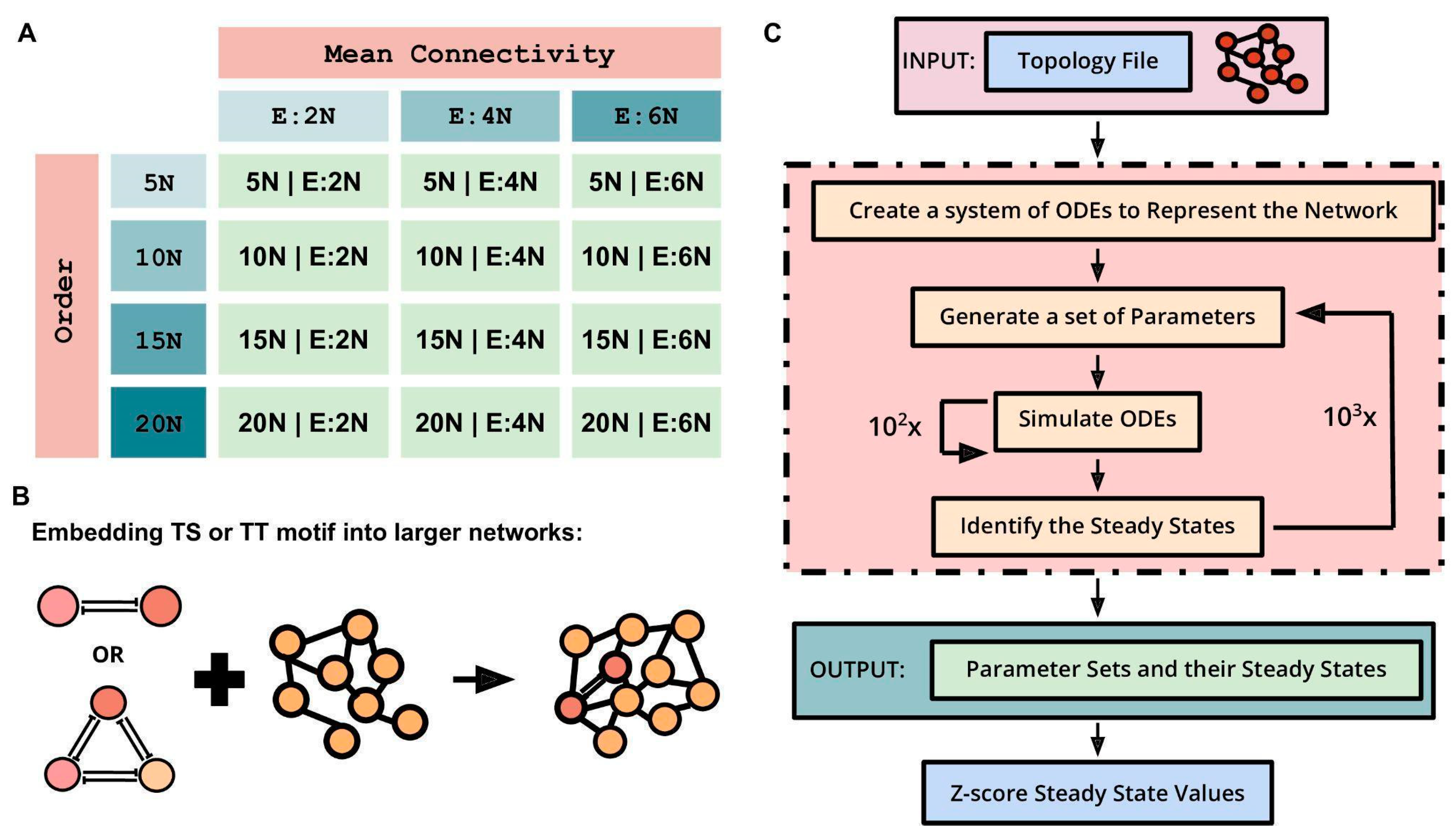
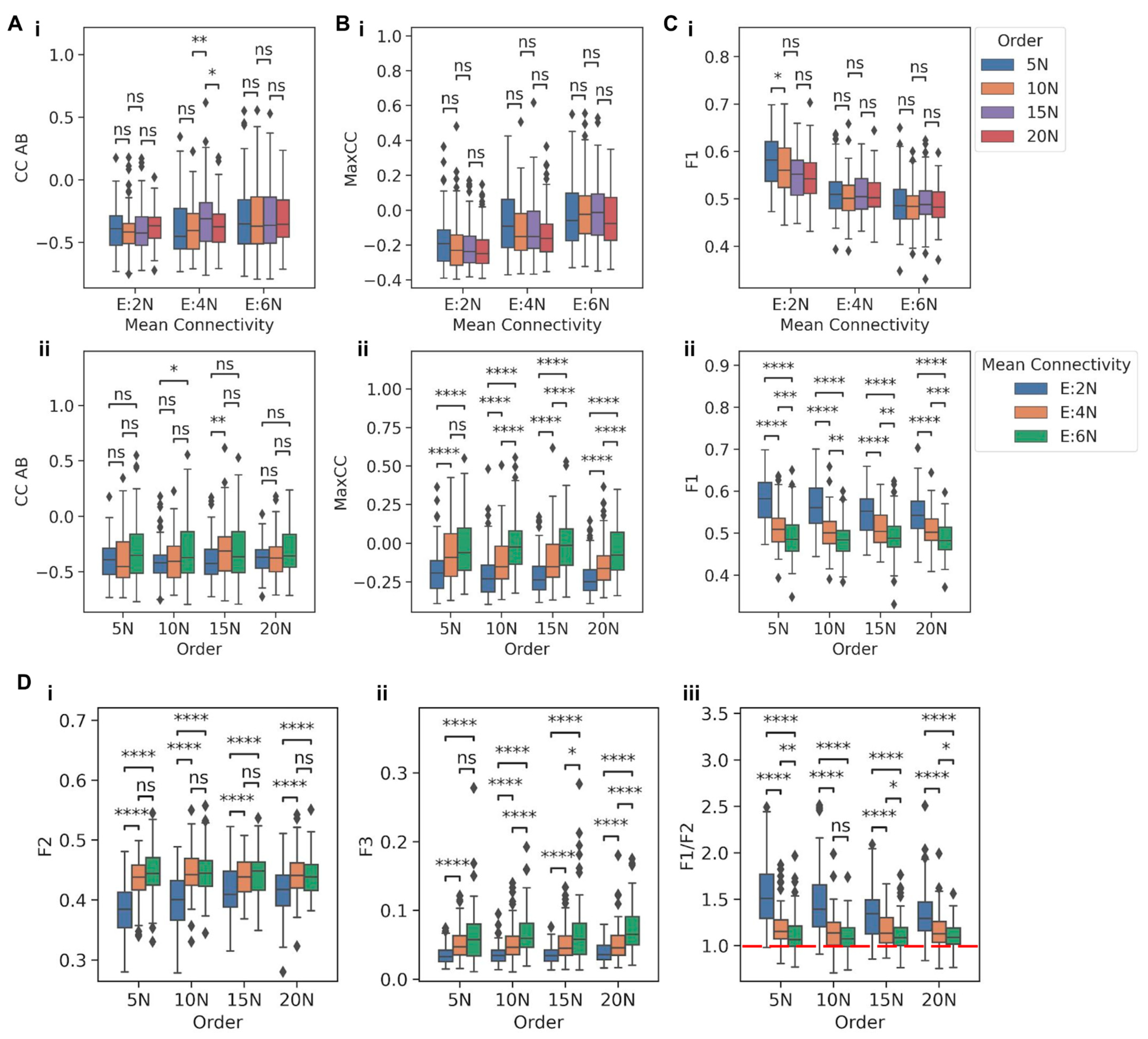
3.2. Functional Traits of Toggle Switch Depend on Density Rather Than the Size of the Larger Networks It Is Embedded in
Next, we embedded TS and TT motifs in different larger networks having combinations of four different network orders and three distinct densities (mean connectivity) to understand how the abovementioned stand-alone dynamic traits of TS and TT change. The four network orders are 5N, 10N, 15N, and 20N, where N is the number of nodes in a network in which these motifs were embedded. Mean connectivity, defined as the ratio of the number of edges to the number of nodes in a network, was used to represent the density of the network. The three mean connectivity values are E:2N, E:4N, and E:6N, where E:xN signifies that the number of edges (E) is x times the number of nodes (N). The combinations of the four network orders (5N, 10N, 15N, and 20N) and three mean connectivity (E:2N, E:4N, and E:6N) resulted in twelve different types of networks (
Figure 2A). For each type of network, n = 100 random network topologies were generated. TS motifs were then embedded into these 1200 (12 types × 100 random networks) randomly generated networks to study the motif’s behavior. For instance, a TS embedded in a 5N, E:4N network will have seven nodes (5 nodes + 2 nodes of TS) and 22 edges (5 × 4 edges + 2 edges of TS) (
Figure 2B). The same process was repeated for the TT motif to generate 1200 random networks. RACIPE was used to simulate the dynamics of these larger networks of varying sizes and mean connectivity, with each network being simulated three times (
Figure 2C). The generated outputs were normalized by Z-scoring and then analyzed to characterize the behavior of TS and TT motifs upon embedding. Three metrics were assessed to quantify the dynamic resilience of TS and TT motifs when embedded in larger networks: bimodality coefficient (BiC), correlation coefficient (CC), and frequency of canonical ‘single-positive’ states as a fraction of all steady states observed (F1).
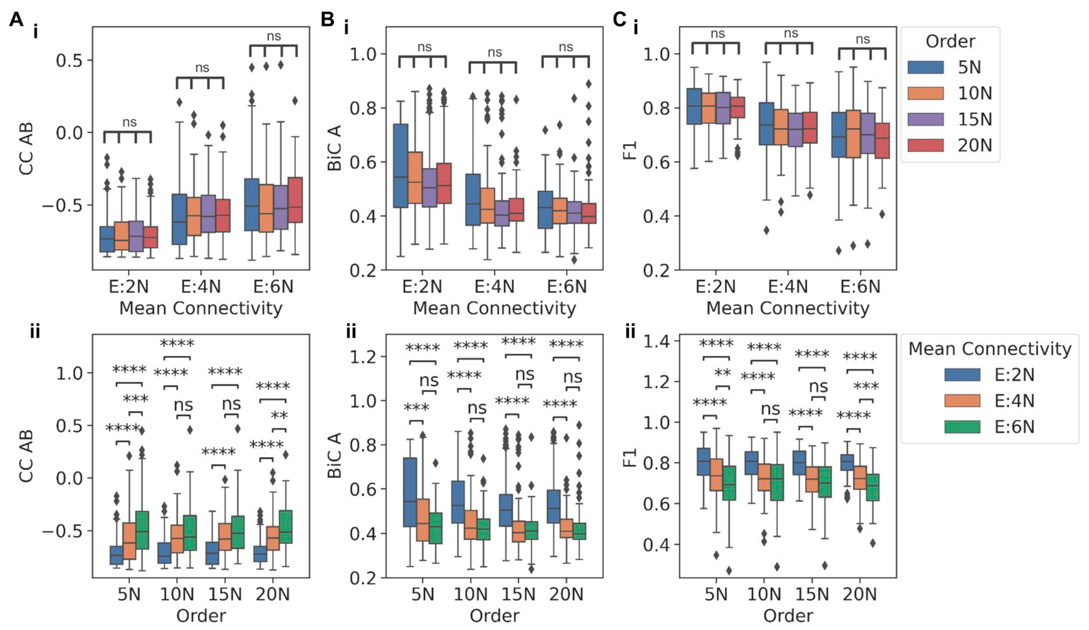
To evaluate how network size and density can independently influence the behavior of a TS when embedded in larger networks of varying orders and mean connectivity, we compared the behavior for networks sharing the same mean connectivity but having different network orders or vice versa. Interestingly, for networks with the same mean connectivity, CC between the two nodes in a TS (CC AB) did not show any significant variation for varied network orders (
Figure 3A(i)). However, when controlling for network order, CC AB reduced as the mean connectivity increased (
Figure 3A(ii)). A similar trend, i.e., the dependence on network density rather than on network size and a decrease in magnitude with increasing network density, was also observed in distributions of BiC values: BiC A and BiC B (
Figure 3B(i,ii) and
Figure S5A(i,ii)) and for F1 (
Figure 3C(i,ii)).
For some cases, the decrease observed in metrics between E:4N and E:6N mean connectivity values was not significantly different, potentially because the TS dynamics were compromised enough in the E:4N case but not in the E:2N case. As a control case, we plotted the distributions of the CC and F1 value for any two randomly chosen nodes which did not belong to the TS motif to compare them with those of TS nodes for networks of order 5N and mean connectivity E:2N. The distributions for the randomly chosen nodes differed significantly when compared to those of the TS nodes (
Figure S5B(i,ii)), showing that the distributions of metrics obtained for TS nodes when embedded were indeed unique to the TS. Put together, all the three metrics considered here to capture the behavior of a TS-CC (how strongly the two nodes in a TS are anti-correlated), BiC (how clearly the high and low levels of a node are segregated), and F1 (how strong is the dominance of mutually exclusivity of the two nodes)—tend to show trends indicating a weakening of the dynamical behavior of a TS, as it is embedded in increasingly denser large networks. In other words, the gradual decrease in a switch-like behavior, as noted through these metrics, is seen in the case of TS being embedded in increasing network density (i.e., mean connectivity) but not in the scenario of increasing network size (order).
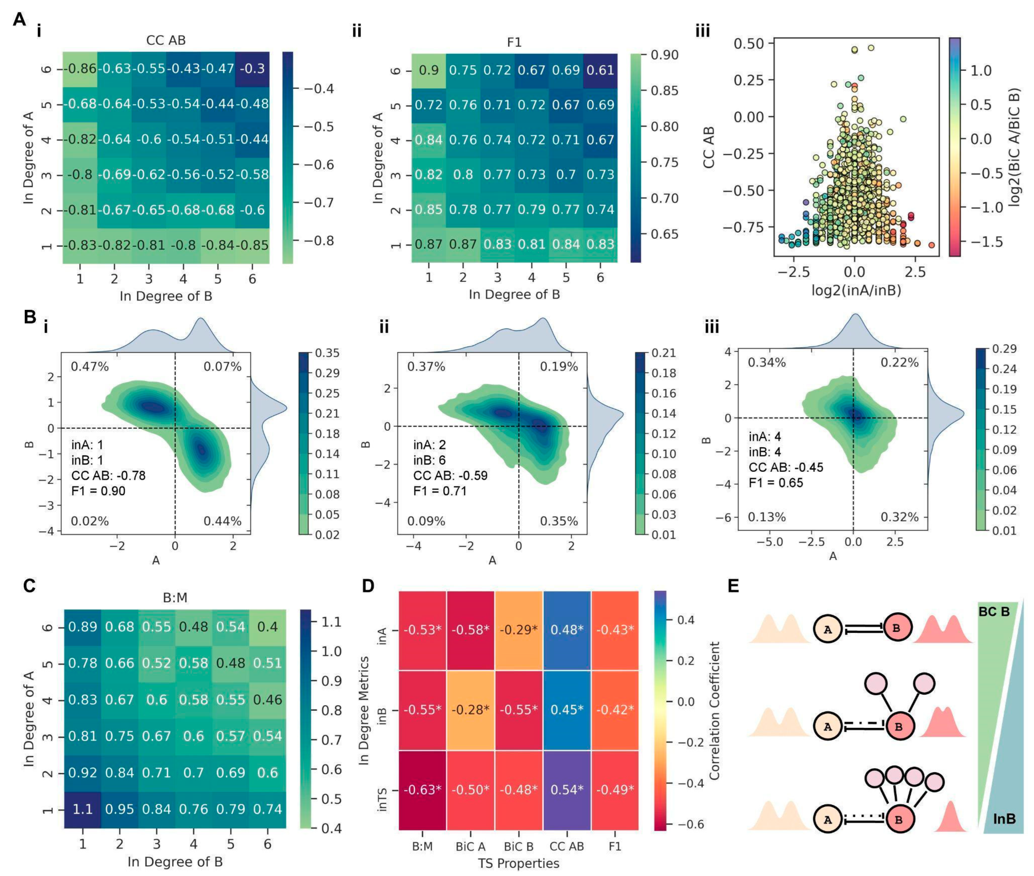
3.3. Local Density around a Toggle Switch Impacts Its Dynamic Behavior
The mean connectivity of a network is the ratio of the total number of edges to the number of nodes in the network, i.e., a measure of global network density. Thus, assuming that the network, on average, is equally sparse or dense, with an increase in mean connectivity of the network, the average in-degree of the nodes of a TS embedded in the network also increases. To ascertain whether this increase in the in-degree (in A and in B) for the TS nodes (as a consequence of the increased mean connectivity of the network) contributed to divergence from stand-alone TS dynamics, we analyzed the variation in the three metrics (CC, BiC, and F1) with a change in the in-degrees of the TS nodes. We observed that as the in-degree of both nodes of a TS increased, the mean CC AB values decreased in magnitude, i.e., the TS nodes A and B were not as strongly negatively correlated with one another as in a stand-alone case (
Figure 4A(i)). For an in-degree of one for both the nodes in a TS, i.e., the case when the two nodes only had outgoing edges apart from their mutual inhibitions, we noticed a mean CC AB value of −0.83 (
Figure 4A(i)), the same as that of an isolated TS motif (
Figure 1B). This trend is observed because the TS in this scenario acts like an independent motif as it is not being affected by the network due lack of incoming edges. Furthermore, the magnitude of CC AB showed the fastest decline when both the nodes had equally increased in degrees (along the diagonal of the heatmap shown in
Figure 4A(i)). Similarly, F1 decreased steadily with in-degrees increasing equally for the two nodes (
Figure 4A(ii)). On the other hand, the BiC of a given node in TS changed only with the in-degree for that node and not with the in-degree for the other node or with the overall in-degree of a TS (
Figure S6A(i,ii)). Additionally, the mean BiC values for nodes with an in-degree more than two were lower than the typical cut-offs considered for bimodality (~0.55), indicating the compromised canonical bimodal distributions observed in the nodes of an isolated TS.
Further, we quantified the impact of asymmetry in terms of incoming edges on a TS by considering the impact of the ratio of in-degree of A to that of B (log
2 (in A/in B)) on CC AB and relative BiC values simultaneously. We noticed that the higher the asymmetry in terms of in-degree (log
2 (in A/in B) > 1 or log
2 (in A/in B) < −1), the stronger the negative correlation between the two TS nodes (CC AB < −0.5) (
Figure 4A(iii)). Importantly, as the magnitude of log
2 (in A/in B) increased, the range of CC AB values (initially even spanning positive values; above the red dotted horizontal line) narrowed to highly negative values close to those observed in isolated TS nodes (−0.83) (
Figure 4A(iii)). Similarly, the value of F1 approached closer to that observed in an isolated TS, as the magnitude of (log
2 (in A/in B)) increased (
Figure S6B(i)). Furthermore, we noted that the higher the in-degree of a node, the more likely it becomes for that node to lose its bimodality seen in a stand-alone TS (log
2 (BiC A/BiC B) < −1 for log
2 (in A /in B) > 1 and log
2 (BiC A/BiC B) > 1 for log
2 (in A/in B) < −1) (
Figure 4A(iii)). Together, this analysis suggests that while F1 (fraction of single positive states) and CC (AB) (correlation coefficient) depend on the in-degree of a TS, the BiC of individual nodes depends on the in-degree of the respective node.
To substantiate this trend further, we investigated representative cases of varied in-degrees of A and B. When the TS has only outgoing connections, and there is no asymmetry between the in-degree of A and B (in A = in B= 1; the only incoming links on A and B are from each other), the bivariate plot of A and B is very similar to that of an isolated TS (compare
Figure 1B with
Figure 4B(i)). However, upon asymmetry in the in-degrees of nodes in a TS (in A = 2, in B = 6, in TS = 2 + 6 = 8), the node with higher in-degree (B) starts to lose its switch-like behavior and shows a more unimodal distribution of its steady state values (
Figure 4B(ii)). However, the strong negative correlation between the TS nodes and, concomitantly, the fraction of “single-positive” states does not decrease as sharply compared to those for the stand-alone case (compare F1 and CC (AB) in
Figure 4B(ii) with those in
Figure 4B(i)). To deconvolute the impact of a higher in-degree of TS vs. asymmetry in the in-degree of both the nodes, we considered a case with the same in-degree for both nodes without changing the net in-degree for a TS (in A = 4, in B = 4, in TS = 4 + 4 =8). Here, the switch-like behavior of both nodes is largely lost, and they show a unimodal distribution of their respective steady-state values (
Figure 4B(iii)). However, CC (AB) and F1 are comparable to the case of asymmetric in-degrees (compare CC (AB) and F1 values in
Figure 4B(ii) with those in
Figure 4B(iii), further supporting that while the higher the in-degree of a toggle switch, the weaker the negative correlation between nodes and the smaller the fraction of “single-positive” states, the bimodality patterns for each node depend on in-degree of that individual node and not on in-degree for TS.
After looking at these representative trends showcasing an increasing in-degree of a node leading to loss of bimodality in steady-state distributions of the corresponding node, we investigated how generic these trends were for embedded TS motifs. We hypothesized that with an increasing in-degree of TS, the frequency of co-occurring ‘single positive’ states (01 and 10 states in a bistable setting) should decrease, with a concomitant increase in having either of these two states, i.e., 01 or 10 states in a monostable setup. This feature can be quantified by the ratio of the fraction of bistable parameter sets showing 01 and 10 steady states to the fraction of monostable parameter sets showing 01 or 10 steady states (B:M). When the TS has only outgoing connections to the network (in A = in B = 1; the only incoming links on A and B are from each other), the B:M ratio is greater than one (
Figure 4C). However, as the in-degree for the TS increases, B:M decreases to values below one, with the sharpest decline when both nodes have equal in-degrees (along the diagonal of the heatmap in
Figure 4C). These results show that as the in-degree of TS increases, the canonical bistable behavior (co-existing ‘single positive’ states) starts to decrease, and simultaneously, the fraction of ‘single-positive’ steady states increases, implying a loss of bistable traits of the TS motif.
Finally, across larger networks of varying sizes and mean connectivity values, we interrogated how in-degrees for individual nodes as well as for a TS (In A, In B, and In TS) correlates with various metrics–F1, CC AB, BiC A, BiC B, and B:M ratio. Net in-degree of the TS (in TS) was found to best explain the decline in the magnitude of CC AB, F1, and the B:M ratio (
Figure 4D). The bimodality coefficients (BiC A and BiC B), on the other hand, were more influenced by the in-degree of their respective nodes and not in TS (
Figure 4D). Therefore, it is the local density on the TS motif (given by in TS) that drives the divergence from TS-like behavior rather than the properties of the whole network in which a TS is embedded.
3.4. In a Toggle Triad, the Fraction of Single-Positive States Captures Its Functional Resilience
After investigating the patterns seen in a TS embedded in large networks, we focused our attempt on understanding the functional resilience of the TT motif. We embedded it into the previously described 12 types of large random networks. Similar to observations in TS, the distributions of pairwise correlation coefficients—CC AB, CC BC, and CC AC—did not show any significant, consistent variation when they were grouped by mean connectivity and compared across the different network orders (
Figure 5A(i) and
Figure S7A(i),B(i)). Intriguingly, unlike the observations in TS, we did not observe any significant differences when the CC values between the TT nodes were grouped by their network orders and compared across the three mean connectivity either (
Figure 5A(ii) and
Figure S7A(ii),B(ii)), despite a visible increase in the range of values. Thus, we investigated how the maximum of the three pairwise correlation values (MaxCC) between the TT nodes—CC AB, CC BC, and CC AC—varied as a function of network order and/or mean connectivity. We observed that when grouped by order, the higher the mean connectivity, the higher the average MaxCC value; however, no such trend was seen when grouped by mean connectivity (
Figure 5B(i,ii)). Reminiscent of observations in TS, the fraction of “single-positive” (010, 100, and 001) steady states (F1) also decreased overall when comparisons were made across their mean connectivity (
Figure 5C(i)), but not across their network orders (
Figure 5C(ii)). Consistently, the fraction of “double-positive” (011, 110, 101) states (F2) and the fraction of “all-positive” or “all-negative” (111, 000) states (F3) increased across different mean connectivity values when grouped by network orders (
Figure 5D(i,ii)), but not when grouped by mean connectivity and compared across network orders. (
Figure S8A(i,ii)). The ratio of the fraction of “single-high” to that of “double-high” states (F1/F2) also showed the same trend, asymptotically reaching the value of one (
Figure 5D(iii) and
Figure S8(iii)). These observations help understand the trend seen for MaxCC tending towards positive values with increasing mean connectivity. With a decreasing frequency of “single-positive” states, the negative pairwise correlation between the TT nodes starts to weaken, and in some cases, one or more of the correlation coefficient values can be positive, suggesting a decay of stand-alone TT dynamics.
To understand if the distributions of MaxCC and F1/F2 values were unique to the TT motif, the distributions of these metrics for TT embedded in 5N and E:2N networks were compared with the distributions of metric values of three randomly chosen nodes which were not a part of the TT motif. We observed that the distributions of both MaxCC (
Figure S9A(i)) and F1/F2 (
Figure S9A(ii)) were significantly different for the randomized nodes when compared to those of TT nodes showing that the distributions of these metrics are indeed unique to TT motif nodes.
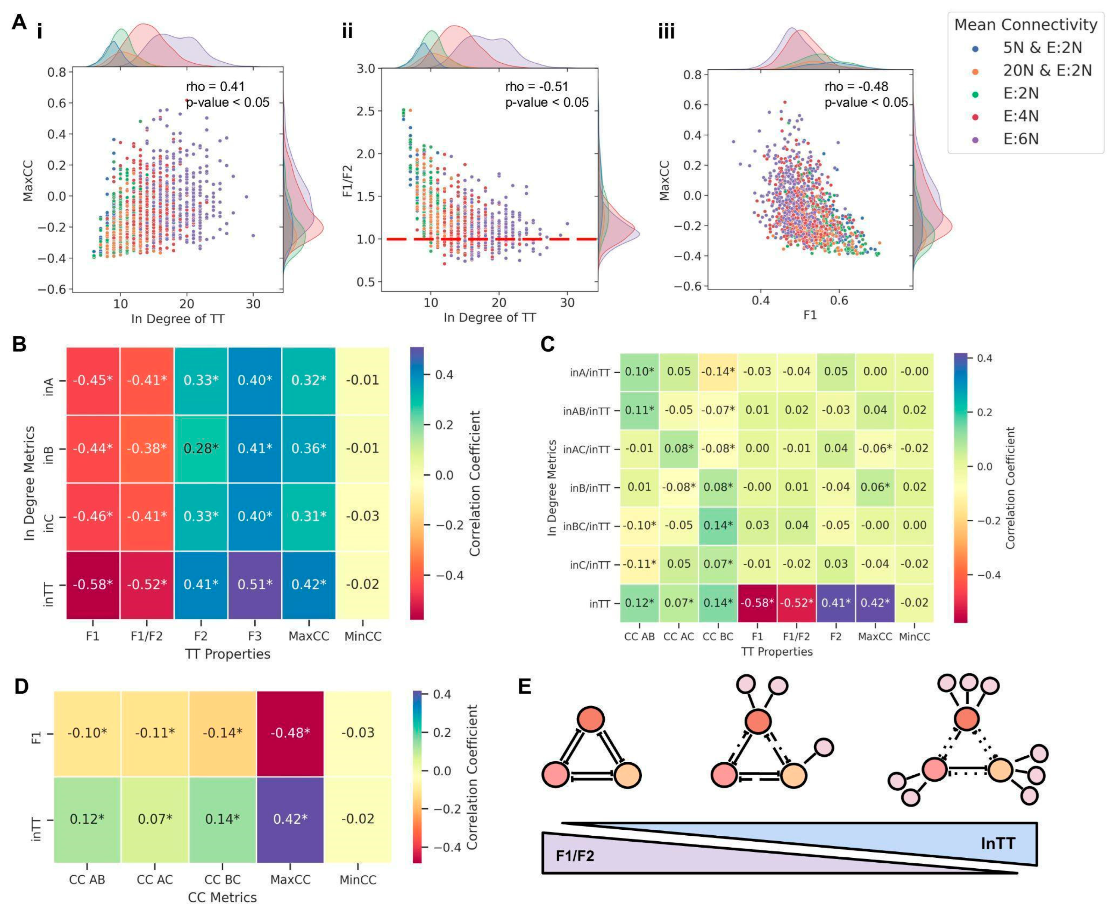
We next investigated how the in-degree of the embedded TT motif affected its behavior. MaxCC values correlated positively (ρ = 0.41,
p < 0.05) with the in-degree of TT, indicating that the higher the in-degree of TT, the stronger the decay of TT dynamics (
Figure 6A(i)). Consistently, F1/F2 values decreased as the in-degree of TT increased (ρ = −0.51,
p < 0.05), tending towards a value of one for high in-degrees of TT (
Figure 6A(ii)), driven by the decrease in F1 and increase in F2 and F3 (
Figure S10A). Moreover, Max CC correlated negatively with F1 (ρ = −0.48,
p < 0.05) and F1/F2 (ρ = −0.45,
p < 0.05) but positively with F2 (ρ = 0.37,
p < 0.05) and F3 (ρ = 0.35,
p < 0.05) (
Figure 6A(iii) and
Figure S10B). Therefore, with an increasing in-degree of a TT, the fraction of “single-positive” states diminishes as they are replaced by “double-positive” (and, to some extent, by “all-positive” or “all-negative”) states. Subsequently, this change in frequencies of different states can weaken the canonical mutual inhibition among nodes in a stand-alone TT, driving one or more pairwise correlation values to be positive, thus validating our choice of Max CC as a metric to assess the decay of TT dynamics.
After characterizing the effect of the net in-degree of TT on its behavior, we investigated how the three pairwise correlations between the TT nodes (CC AB, CC BC, and CC AC) varied with varying in-degrees for the nodes. Unlike the observations for embedded TS, where the CC AB decreased with network mean connectivity and in-degree for motif nodes (
Figure 4A(i) and
Figure S11), the pairwise CCs did not show any discernible trend in an embedded TT; therefore, we excluded them from any further analysis. On the other hand, F1, F2, and F3 changed significantly as the in-degrees of any two nodes in the TT increased (F1 decreased while F2 and F3 increased); at high in-degrees for any two nodes, F2 is approximately equal to F1 and six to seven times the corresponding F3 values (
Figure S12). Next, we quantified changes in these metrics brought about by simultaneously varying the in-degree of the third node as well. An increase in C, while maintaining the values of in A and in B, led to a lower F1, higher F2, and F3 values, as expected (compare corresponding cells in
Figure S13B with Figure S13A), thereby showcasing the impact of increasing net in-degree on the breakdown of stand-alone TT dynamics.
Because pairwise correlation coefficients between TT nodes were unable to gauge the changes in TT dynamics, we performed multiple linear regression (MLR) on steady-state values of the TT nodes to understand the changes in inter-node dependence brought about by embedding the TT. MLR was performed by taking steady-state values of A and B as independent variables and steady states of C as the dependent variable. The distributions of coefficients of A and B (ACoeff and BCoeff, respectively, i.e., the slopes of the regression plane) and the model’s scores (R
2 values) were then compared across network orders by grouping them according to common mean connectivity and vice versa. As the mean connectivity of the network increased, the magnitude of the mean values of ACoeff and BCoeff decreased, indicating that the repressing effect of the two nodes on C decreased as the network density increased (
Figure S14A,B(i,ii)). Furthermore, the scores of MLR models declined as the mean connectivity of the network increased, pointing towards a decline in the predictive power of the MLR model as the TT dynamics deviated from their canonical behavior with the increasing network density (
Figure S14A(iii),B(iii)). Further, the higher the in-degree of TT, the lower the model’s score and the magnitudes of ACoeff and BCoeff values (
Figure S14C), reiterating the disruptive impact of the in-degree of TT on its canonical behavior. Intriguingly, for E:6N, we noticed some ACoeff and BCoeff values to be positive (
Figure S14C), reminiscent of MaxCC values also becoming greater than zero for high mean connectivity (
Figure 6A(iii)).
Next, we performed a meta-analysis across network orders and mean connectivity in terms of correlation of various metrics with the in-degree of individual nodes as well as the net in-degree of TT. With all metrics considered here (F1, F2, F3, Max CC, F1/F2), In TT showed a stronger correlation (ρ > 0 for F2, F3; ρ < 0 for F1, F2/F2, MaxCC) than the in-degree of any of the individual nodes (in A, in B, in C), indicating that net in-degree was the best predictor of embedded TT dynamics. (
Figure 6B), and reinforcing the trends seen in embedded TS (
Figure 4D). This trend was consistent even when the individual in-degree or combined in-degree of two nodes, normalized by net in-degree (in A/in TT, in B/in TT, in C/in TT, in AB/in TT, in BC/in TT, in AC/in TT) was considered (
Figure 6C). Intriguingly, while TT correlated strongly with MaxCC (i.e., the pair of nodes whose “mutual exclusion” is the weakest), it did not correlate as strongly with individual pairwise correlation coefficients (CC AB, CC BC, CC AC) (
Figure 6C). Furthermore, while MaxCC correlated strongly with individual in-degree as well as with net in-degree, Min CC (the minimum value among three pairwise correlation coefficients, i.e., the pair of nodes showing the strongest mutual inhibition properties) did not show any such association (
Figure 6B,C). This difference in terms of MaxCC vs. MinCC is consistent with observations that all three individual pairwise correlation coefficients show only a weak correlation with both in-degree of TT and with F1 (
Figure 6D), thus justifying our choice of using MaxCC as a metric to track the dynamics of embedded TT.
Put together, these results highlight that while the total in-degree of a TT motif is a good indicator of the decay of TT dynamics (decrease in “single-positive” states and simultaneous increase in “double-positive”), it often does not contain precise information on which out of the three possible pairs of nodes in a TT have their mutual repression compromised and thus drive a decay in the stand-alone dynamical behavior of a TT. Despite this limitation, similar to the results seen for TS, the dynamics of embedded TT were determined not by network order, network density, or individual in-degrees of the motif nodes but by the total in-degree of the motif (In TT) (
Figure 6E). Moreover, both for the TS and TT motifs, the nature of these in-degrees—being either activating or repressing—did not affect the nature of divergence from canonical behavior (
Figure S15), highlighting that the motif is sensitive to the total number of incoming edges, not their distributions in terms of their sign/effect.
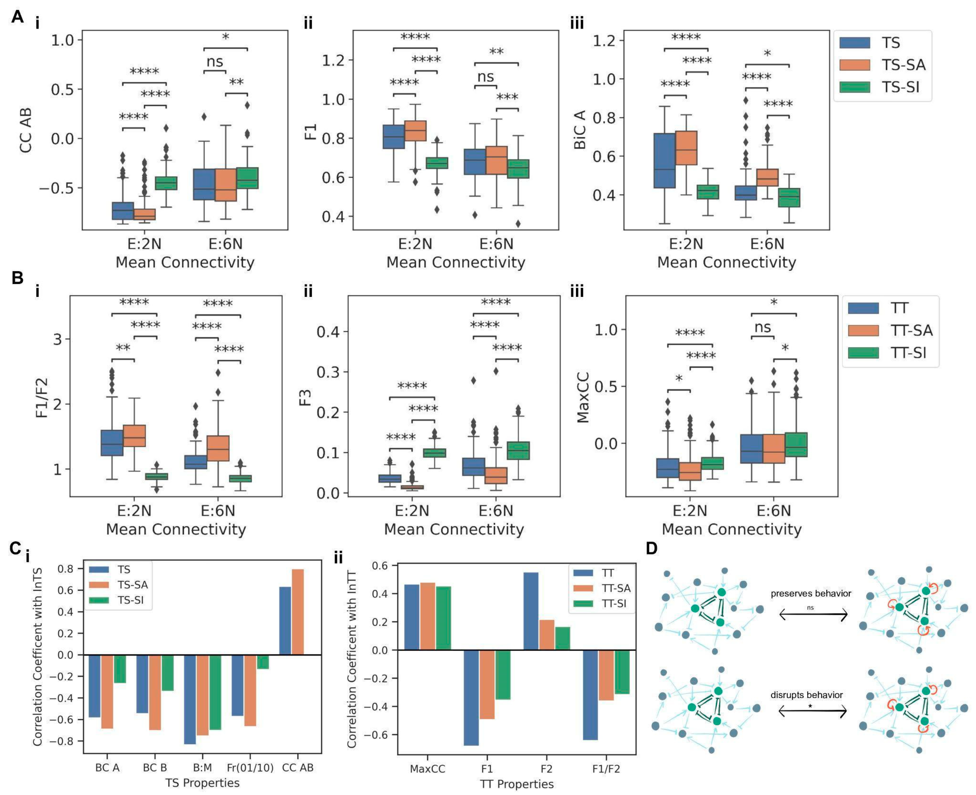
3.5. Effect of Self-Activation and Self-Inhibition of Nodes on the Modularity of Motifs
Many “master regulators” involved in driving cell fate decisions form TS or TT motifs, such as PU.1 and GATA1 in hematopoietic stem cells, and CDX2 and OCT4 in embryonic stem cells can also self-activate to stabilize an “undecided” multipotent state characterized by promiscuous expression of motif nodes [
2,
13]. In order to evaluate the effects of such self-activations and self-inhibitions on the motif nodes, the TS and TT motifs containing self-activation (TS-SA and TT-SA) and self-inhibition edges (TS-SI and TT-SI) on all nodes were embedded into combinations of two network orders (5N and 20N) and two mean connectivity (E:2N and E:6N), resulting in four types of networks. The same pipeline as before was followed to generate the networks, with n = 100 for each type of network (i.e., 400 networks per motif). The motifs TS-SA, TS-SI, TT-SA, and TT-SI were then embedded into these networks and simulated with RACIPE, and corresponding metrics were compared. First, we compared the TS, TS-SA, and TS-SI embedded in networks having the same mean connectivity. For all three metrics (CC AB, F1, and BiC), TS, TS-SA, and TS-SI showed significantly different distributions (
Figure 7A(i–iii)). While including self-activation moderately strengthened the correlation between A and B, self-inhibition significantly weakened it (
Figure 7A(i)). Similarly, while including self-activation led to slightly increased F1, and BiC values, conversely, including self-inhibition on TS nodes reduced the F1 and BiC values (
Figure 7A(ii,iii)). These results suggest that while adding self-activation on nodes can preserve the dynamical features of a TS embedded in large networks, self-inhibition can accelerate the decay of TS dynamics, possibly offering a reason for an observed higher frequency of self-activating ‘master regulators’ rather than the self-inhibiting ones [
25].
Next, we probed the impact of self-activation and self-inhibition in the case of an embedded TT. Similar to observations in TS, self-inhibition had an opposite and a stronger impact in influencing the metrics as compared to self-activation. Median F1/F2 values noted for TT-SA were higher than those for both TT and TT-SI, irrespective of the mean connectivity (
Figure 7B(i)). Consistently, median F3 values are higher for TT-SI than for TT and TT-SA (
Figure 7B(ii)). Together, these results indicate that while adding self-activation on nodes of a TT can enrich for canonical “single-positive states”, adding self-inhibition can enrich for “all-positive” or “all-negative” states instead. Similarly, for Max CC, TT-SI had higher median values than both TT and TT-SA cases (
Figure 7B(iii)), resulting in a faster decay of canonical properties of TT. In other words, the self-inhibiting “master regulators” can exhibit compromised phenotypic decision-making as compared to non-self-inhibiting ones.
The effect of the addition of self-activation and self-inhibition edges on the nodes of the motifs was also gauged by embedding the motif, its self-activation, and self-inhibition version in the same ensemble of random networks having network orders 5N and mean connectivity of E:2N and E:6N (
Figure S16A). These networks were then simulated using RACIPE [
23]. The metrics of both the motifs showed significantly different distributions when grouped by common network mean connectivity (
Figure S16B(i–iii),C(i,ii)). A similar trend of the addition of self-activation leading to preserving and the addition of self-inhibition leading to a decay in the dynamical properties of motifs was observed. This trend was also reflected in the ratios of the metric values of TT-SA or TT-SI motifs to the corresponding metric values of TT motifs embedded in the same larger network (
Figure S16C(iii)), indicating that the addition of self-activation led to a decay of the dynamical properties even when the larger networks in which the motifs were embedded were maintained to be the same.
Finally, we assessed whether adding self-regulation preserves the correlation of the in-degree of the motif (TS or TT) with various metrics (BiC A, BiC B, B:M, F1 and CC AB for TS; F1, F2, F1/F2 and MaxCC for TT). We consistently observed that motifs with self-inhibition had a lower magnitude of correlation with all these motif properties as compared to motifs with no self-regulation or with self-activation (
Figure 7C(i,ii)), indicating a faster loss and subsequent saturation of the motif’s dynamical properties. These trends reaffirm that the addition of self-activating loops preserves the canonical behavior of the motif while adding self-inhibition loops diminishes it remarkably (
Figure 7D).


 ,
, 


