

Application of the Dynamical Network Biomarker Theory to Raman Spectra

 , , , , , , , , , and
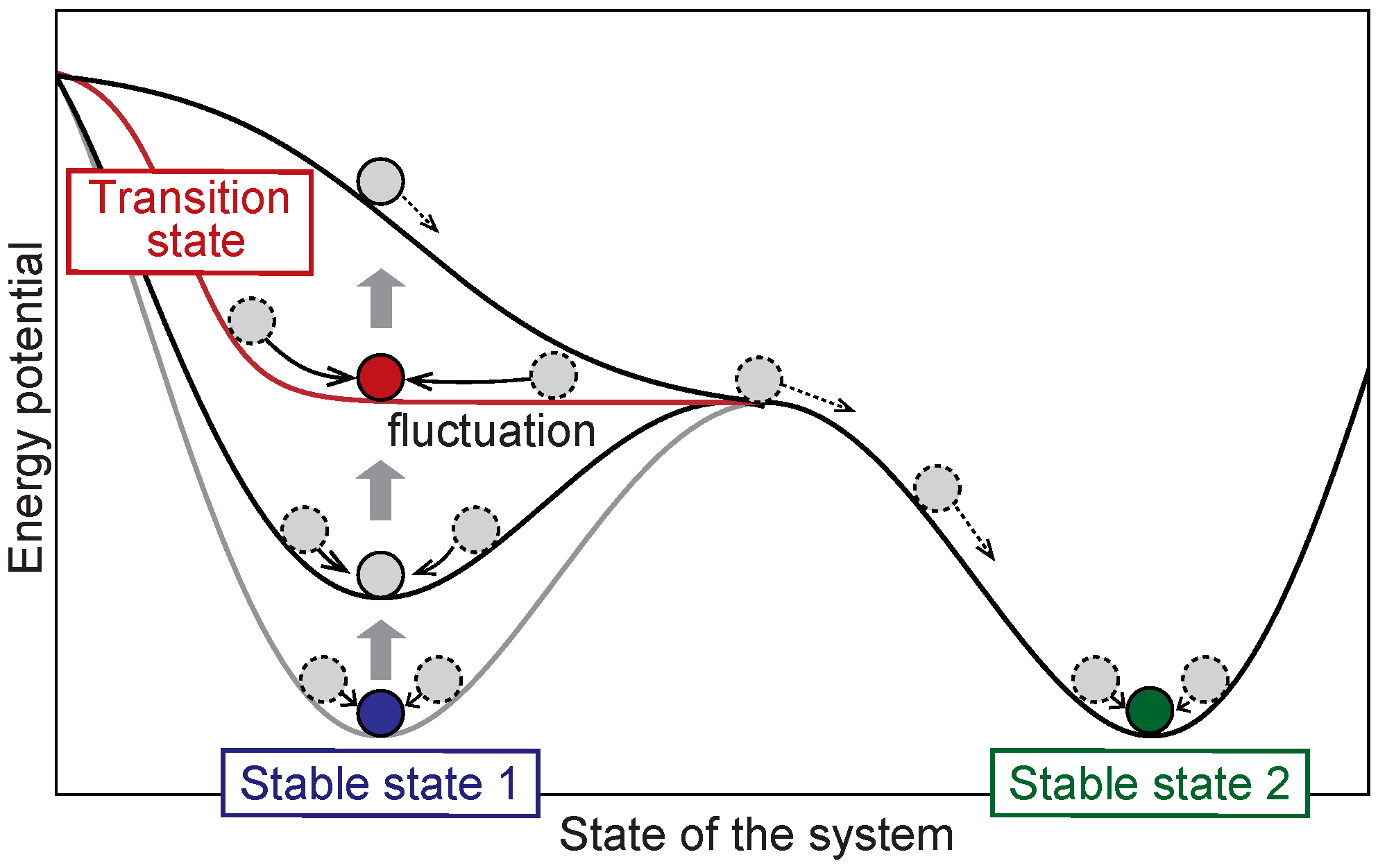
Abstract
1. Introduction
2. Materials and Methods
2.1. Overview of the DNB Theory
- Preprocessing;
- F-test for the evaluation of fluctuations;
- Correlations to evaluate the relationships between fluctuating variables;
- Clustering to define DNB candidates;
- DNB scores to identify the transition state and DNB elements.
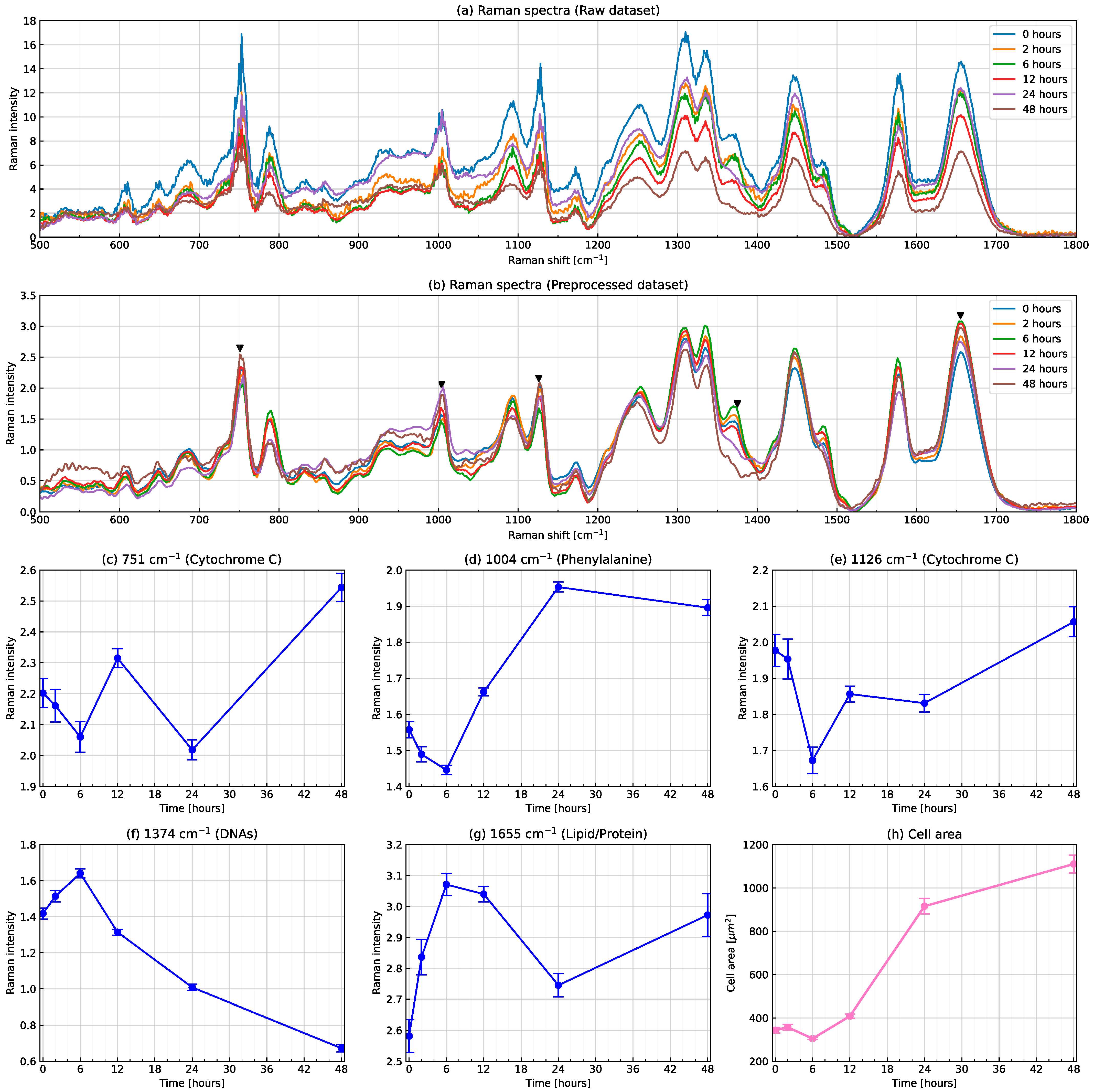
2.2. Raman Spectra of the T Cell Activation Process
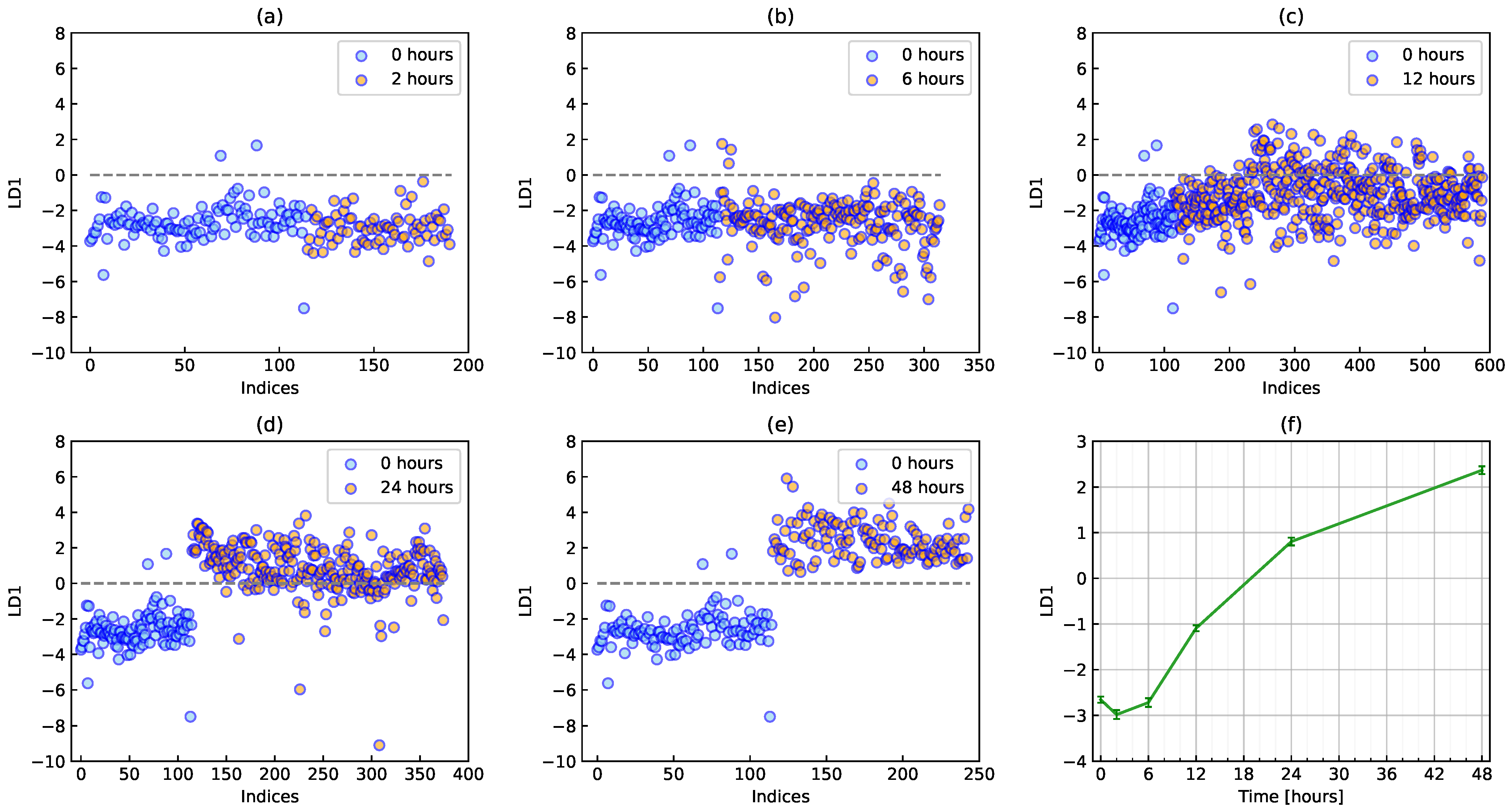
2.3. PCA-LDA
2.4. A DNB Analysis Suitable for Raman Spectra
3. Results and Discussion
3.1. Conventional Analysis
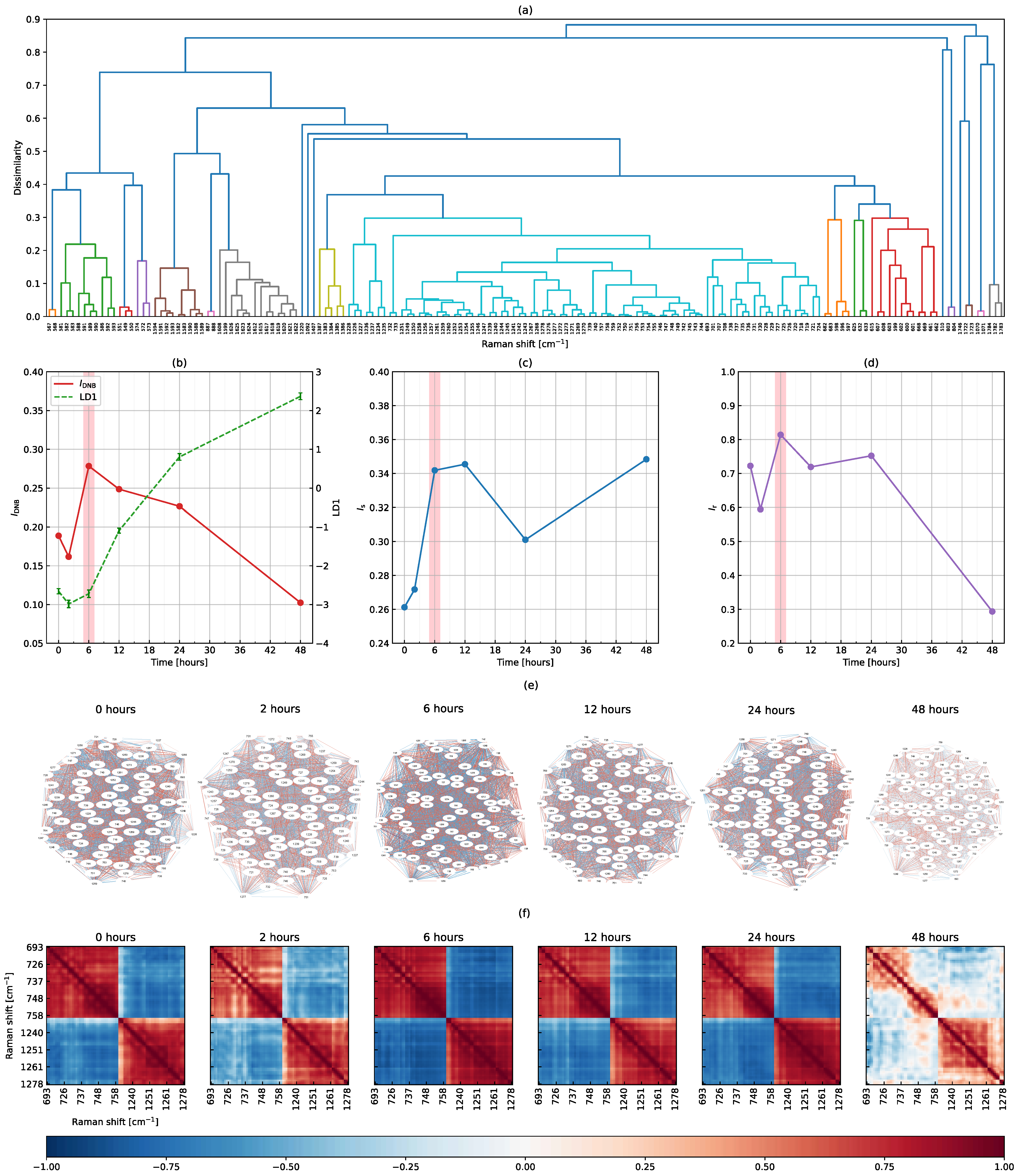
3.2. The DNB Analysis Using Full-Range Raman Shifts
3.3. The DNB Analysis Using Peak-Filtering Raman Shifts
4. Conclusions
Author Contributions
Funding
Data Availability Statement
Conflicts of Interest
References
- Chen, L.; Liu, R.; Liu, Z.P.; Li, M.; Aihara, K. Detecting early-warning signals for sudden deterioration of complex diseases by dynamical network biomarkers. Sci. Rep. 2012, 2, 342. [Google Scholar] [CrossRef] [PubMed]
- Aihara, K.; Liu, R.; Koizumi, K.; Liu, X.; Chen, L. Dynamical network biomarkers: Theory and applications. Gene 2022, 808, 145997. [Google Scholar] [CrossRef]
- Carpenter, S.R.; Brock, W.A. Rising variance: A leading indicator of ecological transition. Ecol. Lett. 2006, 9, 311–318. [Google Scholar] [CrossRef] [PubMed]
- Dakos, V.; Scheffer, M.; van Nes, E.H.; Brovkin, V.; Petoukhov, V.; Held, H. Slowing down as an early warning signal for abrupt climate change. Proc. Natl. Acad. Sci. USA 2008, 105, 14308–14312. [Google Scholar] [CrossRef] [PubMed]
- Scheffer, M.; Bascompte, J.; Brock, W.A.; Brovkin, V.; Carpenter, S.R.; Dakos, V.; Held, H.; van Nes, E.H.; Rietkerk, M.; Sugihara, G. Early-warning signals for critical transitions. Nature 2009, 461, 53–59. [Google Scholar] [CrossRef]
- Moon, H.; Lu, T.C. Network catastrophe: Self-organized patterns reveal both the instability and the structure of complex networks. Sci. Rep. 2015, 5, 9450. [Google Scholar] [CrossRef]
- Veraart, A.J.; Faassen, E.J.; Dakos, V.; van Nes, E.H.; Lürling, M.; Scheffer, M. Recovery rates reflect distance to a tipping point in a living system. Nature 2012, 481, 357–359. [Google Scholar] [CrossRef]
- Liu, R.; Li, M.; Liu, Z.-P.; Wu, J.; Chen, L.; Aihara, K. Identifying critical transitions and their leading biomolecular networks in complex diseases. Sci. Rep. 2012, 2, 813. [Google Scholar] [CrossRef]
- Chen, P.; Liu, R.; Li, Y.; Chen, L. Detecting critical state before phase transition of complex biological systems by hidden Markov model. Bioinformatics 2016, 32, 2143–2150. [Google Scholar] [CrossRef]
- Liu, R.; Yu, X.; Liu, X.; Xu, D.; Aihara, K.; Chen, L. Identifying critical transitions of complex diseases based on a single sample. Bioinformatics 2014, 30, 1579–1586. [Google Scholar] [CrossRef]
- Liu, X.; Liu, R.; Zhao, X.-M.; Chen, L. Detecting early-warning signals of type 1 diabetes and its leading biomolecular networks by dynamical network biomarkers. BMC Med. Genom. 2013, 6, S8. [Google Scholar] [CrossRef] [PubMed]
- Li, M.; Zeng, T.; Liu, R.; Chen, L. Detecting tissue-specific early warning signals for complex diseases based on dynamical network biomarkers: Study of type 2 diabetes by cross-tissue analysis. Brief Bioinform. 2014, 15, 229–243. [Google Scholar] [CrossRef] [PubMed]
- Koizumi, K.; Oku, M.; Hayashi, S.; Inujima, A.; Shibahara, N.; Chen, L.; Igarashi, Y.; Tobe, K.; Saito, S.; Kadowaki, M.; et al. Identifying pre-disease signals before metabolic syndrome in mice by dynamical network biomarkers. Sci. Rep. 2019, 9, 8767. [Google Scholar] [CrossRef] [PubMed]
- Yang, B.; Li, M.; Tang, W.; Liu, W.; Zhang, S.; Chen, L.; Xia, J. Dynamic network biomarker indicates pulmonary metastasis at the tipping point of hepatocellular carcinoma. Nat. Commun. 2018, 9, 678. [Google Scholar] [CrossRef] [PubMed]
- Liu, X.; Chang, X.; Leng, S.; Tang, H.; Aihara, K.; Chen, L. Detection for disease tipping points by landscape dynamic network biomarkers. Natl. Sci. Rev. 2019, 6, 775–785. [Google Scholar] [CrossRef]
- Ge, J.; Song, C.; Zhang, C.; Liu, X.; Chen, J.; Dou, K.; Chen, L. Personalized Early-Warning Signals during Progression of Human Coronary Atherosclerosis by Landscape Dynamic Network Biomarker. Genes 2020, 11, 676. [Google Scholar] [CrossRef]
- Zhang, C.; Zhang, H.; Ge, J.; Mi, T.; Cui, X.; Tu, F.; Gu, X.; Zeng, T.; Chen, L. Landscape dynamic network biomarker analysis reveals the tipping point of transcriptome reprogramming to prevent skin photodamage. J. Mol. Cell Biol. 2022, 13, 822–833. [Google Scholar] [CrossRef]
- Kamal, M.A.S.; Oku, M.; Hayakawa, T.; Imura, J.; Aihara, K. Early detection of a traffic flow breakdown in the freeway based on dynamical network markers. Int. J. ITS Res. 2020, 18, 422–435. [Google Scholar] [CrossRef]
- Okada, M.; Smith, N.I.; Palonpon, A.F.; Endo, H.; Kawata, S.; Sodeoka, M.; Fujita, K. Label-free Raman observation of cytochrome c dynamics during apoptosis. Proc. Natl. Acad. Sci. USA 2012, 109, 28–32. [Google Scholar] [CrossRef]
- Ichimura, T.; Chiu, L.D.; Fujita, K.; Kawata, S.; Watanabe, T.M.; Yanagida, T.; Fujita, H. Visualizing Cell State Transition Using Raman Spectroscopy. PLoS ONE 2014, 9, 84478. [Google Scholar] [CrossRef]
- Ichimura, T.; Chiu, L.D.; Fujita, K.; Machiyama, H.; Kawata, S.; Watanabe, T.M.; Fujita, H. Visualizing the appearance and disappearance of the attractor of differentiation using Raman spectral imaging. Sci. Rep. 2015, 5, 11358. [Google Scholar] [CrossRef] [PubMed]
- Ichimura, T.; Chiu, L.D.; Fujita, K.; Machiyama, H.; Yamaguchi, T.; Watanabe, T.M.; Fujita, H. Non-label immune cell state prediction using Raman spectroscopy. Sci. Rep. 2016, 6, 37562. [Google Scholar] [CrossRef]
- Chaudhary, N.; Nguyen, T.N.Q.; Cullen, D.; Meade, A.D.; Wynne, C. Discrimination of immune cell activation using Raman micro-spectroscopy in an in-vitro & ex-vivo model. Spectrochim. Acta Part A 2021, 248, 119118. [Google Scholar]
- Taketani, A.; Andriana, B.B.; Matsuyoshi, H.; Sato, H. Raman endoscopy for monitoring the anticancer drug treatment of colorectal tumors in live mice. Analyst 2017, 142, 3680–3688. [Google Scholar] [CrossRef] [PubMed]
- Ishimaru, Y.; Oshima, Y.; Imai, Y.; Iimura, T.; Takanezawa, S.; Hino, K.; Miura, H. Raman spectroscopic analysis to detect reduced bone quality after sciatic neurectomy in mice. Molecules 2018, 23, 3081. [Google Scholar] [CrossRef]
- Ogawa, K.; Oshima, Y.; Etoh, T.; Kaisyakuji, Y.; Tojigamori, M.; Ohno, Y.; Shiraishi, N.; Inomata, M. Label-free detection of human enteric nerve system using Raman spectroscopy: A pilot study for diagnosis of Hirschsprung disease. J. Pediatr. Surg. 2021, 56, 1150–1156. [Google Scholar] [CrossRef] [PubMed]
- Guleken, Z.; Bulut, H.; Bulut, B.; Paja, W.; Parlinska-Wojtan, M.; Depciuch, J. Correlation between endometriomas volume and Raman spectra. Attempting to use Raman spectroscopy in the diagnosis of endometrioma. Spectrochim. Acta A Mol. Biomol. Spectrosc. 2022, 274, 121119. [Google Scholar] [CrossRef] [PubMed]
- Guleken, Z.; Kula-Maximenko, M.; Depciuch, J.; Kılıç, A.M.; Sarıbal, D. Detection of the chemical changes in blood, liver and brain caused by electromagnetic field exposure using Raman spectroscopy, biochemical assays combined with multivariate analyses. Photodiagn. Photodyn. Ther. 2022, 38, 102779. [Google Scholar] [CrossRef]
- Nakagawa, T.; Oku, M.; Aihara, K. Early warning signals by dynamical network markers. Seisan Kenkyu 2016, 68, 271–274. [Google Scholar]
- Otsu, N. A Threshold Selection Method from Gray-Level Histograms. IEEE Trans. Syst. Man Cybern. 1979, 9, 62–66. [Google Scholar] [CrossRef]
- Mikhailyuk, I.K.; Razzhivin, A.P. Background Subtraction in Experimental Data Arrays Illustrated by the Example of Raman Spectra and Fluorescent Gel Electrophoresis Patterns. Instrum. Exp. Tech. 2003, 46, 765–769. [Google Scholar] [CrossRef]
- Movasaghi, Z.; Rehman, S.; Rehman, I.U. Raman Spectroscopy of Biological Tissues. Appl. Spectrosc. Rev. 2007, 42, 493–541. [Google Scholar] [CrossRef]


Publisher’s Note: MDPI stays neutral with regard to jurisdictional claims in published maps and institutional affiliations. |
© 2022 by the authors. Licensee MDPI, Basel, Switzerland. This article is an open access article distributed under the terms and conditions of the Creative Commons Attribution (CC BY) license (https://creativecommons.org/licenses/by/4.0/).
Share and Cite
Haruki, T.; Yonezawa, S.; Koizumi, K.; Yoshida, Y.; Watanabe, T.M.; Fujita, H.; Oshima, Y.; Oku, M.; Taketani, A.; Yamazaki, M.; et al. Application of the Dynamical Network Biomarker Theory to Raman Spectra. Biomolecules 2022, 12, 1730. https://doi.org/10.3390/biom12121730
Haruki T, Yonezawa S, Koizumi K, Yoshida Y, Watanabe TM, Fujita H, Oshima Y, Oku M, Taketani A, Yamazaki M, et al. Application of the Dynamical Network Biomarker Theory to Raman Spectra. Biomolecules. 2022; 12(12):1730. https://doi.org/10.3390/biom12121730
Chicago/Turabian StyleHaruki, Takayuki, Shota Yonezawa, Keiichi Koizumi, Yasuhiko Yoshida, Tomonobu M. Watanabe, Hideaki Fujita, Yusuke Oshima, Makito Oku, Akinori Taketani, Moe Yamazaki, and et al. 2022. "Application of the Dynamical Network Biomarker Theory to Raman Spectra" Biomolecules 12, no. 12: 1730. https://doi.org/10.3390/biom12121730
APA StyleHaruki, T., Yonezawa, S., Koizumi, K., Yoshida, Y., Watanabe, T. M., Fujita, H., Oshima, Y., Oku, M., Taketani, A., Yamazaki, M., Ichimura, T., Kadowaki, M., Kitajima, I., & Saito, S. (2022). Application of the Dynamical Network Biomarker Theory to Raman Spectra. Biomolecules, 12(12), 1730. https://doi.org/10.3390/biom12121730