Machine Learning Approaches for Quality Assessment of Protein Structures


Abstract
1. Introduction
2. Background
2.1. Machine Learning and Deep Learning
2.2. Protein Structure Prediction
2.3. Critical Assessment of Structure Prediction
2.4. Metrics
- The GDT is a rigid-body measure that identifies the largest subset of model residues that can be superimposed on the corresponding residues in the reference structure within a specific distance threshold [63]. The average GDT score (GDT_TS) within the specific distance thresholds provides a single measure of the overall model accuracy: [64]:where is the predicted model, is the reference model, and , , , and are the percentages of atoms of that can be superposed on the atoms of [65] within 1, 2, 4, and 8Å, respectively. The score lies between zero (no superposition) and one (total superposition).
- TM-score [66]:The TM-score of a structural model is based on the alignment coverage and the accuracy of the aligned residue pairs. This score employs a distance-dependent weighting scheme that favors the correctly predicted residues and penalizes the poorly aligned residues [67]. To eliminate the protein size dependency, the final score is normalized by the size of the protein. The TM-score lies between zero (no match) and one (perfect match) and is calculated as follows:with:Here, and are the lengths of the aligned protein and native structure, respectively. ) is a distance scale that normalizes , the distance between a residue in the target protein and the corresponding residue in the aligned protein. The TM-score provides a more accurate quality estimate than GDT_TS on full-length proteins [66].
- lDDT (LDDT in CASP) [65]:The lDDT score compares the environment of all atoms in a model to those in the reference structure, where the environment refers to the existence of certain types of atoms within a threshold. lDDT is advantaged by being superposition free. To compute the lDDT, the distances between all pairs of atoms lying within the predefined threshold are recorded for the reference structure. If the distances between each atom pair are similar in the model and the reference, this distance is considered to be preserved. The final lDDT score averages the fractions of the preserved distances over four predefined thresholds: 0.5Å, 1Å, 2Å, and 4Å [68]. The lDDT score is highly sensitive to local atomic interactions, but insensitive to domain movements.
- CAD score [63]:The CAD score estimates the quality of a model by computing its interatomic-contact difference from the reference structure. The formulae are as follows:where i and j represent the residues in the predicted model and the reference protein structure, respectively, and G is the set of contacting residue pairs in the reference structure. and denote the contact areas in the reference structure and the predicted model, respectively. If a pair of contacting residues exists in the reference model, but not in the predicted model, that pair is excluded from set G. Similarly, if two residues contact in the predicted model, but are missing from the reference model, the contact area is regarded as zero. The CAD score ranges from zero (no similarity between the predicted and actual model structures) and one (perfect match of the predicted and actual structures).
2.5. Features
2.6. Data Sources
2.7. K-Fold Cross-Validation
3. ML-Based EMA Methods
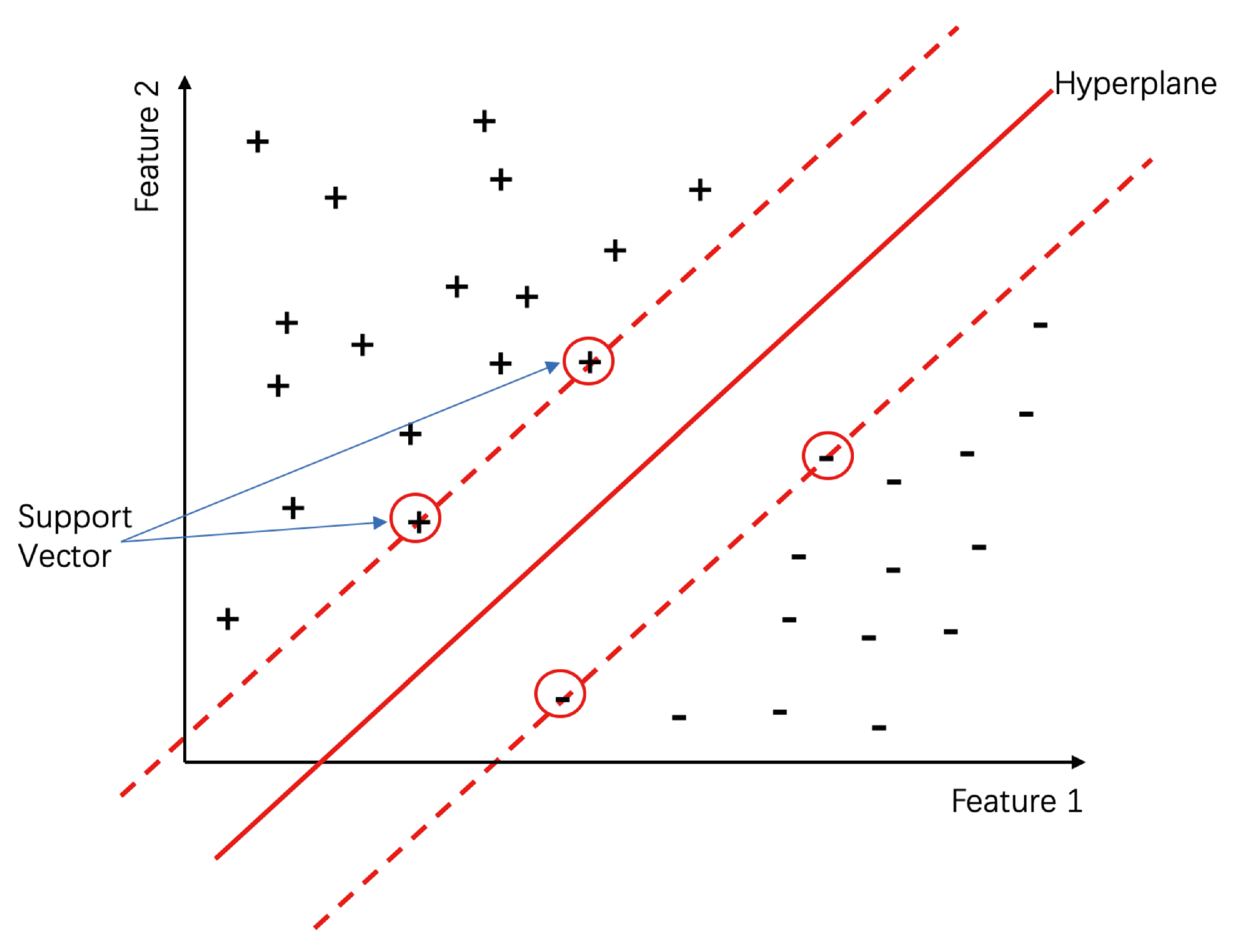
3.1. Support Vector Machine
- ProQ is a series of methods for EMA. ProQ2 selects the linear kernel function and a handful of structural and sequence-derived features. The former describes the local environment around each residue, whereas the latter predicts the secondary structure, surface exposure, conservation, and other relevant features [33]. ProQ3 inherits all the features of ProQ2, and adopts two new features based on Rosetta energy terms [22], namely the full-atom Rosetta energy terms and the coarse-grained centroid Rosetta energy terms. ProQ3 was trained on CASP9 and tested on CASP11 and CAMEO. ProQ3 outperforms ProQ2 in correlation and achieves the highest average GDT_TS score on both the CAMEO and CASP11 datasets [22].
- SVMQA [23]SVMQA inputs eight potential energy-based terms and 11 consistency-based terms (for assessing the consistency between the predicted and actual models) and predicts the TM-score and GDT_TS score [23]. This model was trained on CASP8 and CASP9 and validated on CASP10. In an experimental evaluation, SVMQA was the highest performing single-model MQA method at that time. The biggest innovation in this method is the incorporation of the random forest (RF) algorithm for feature importance estimation [23]. The features with higher importance are selected as the input parameters. Moreover, the quality score can be changed by varying the feature combinations. The TM-score (SVMQA_TM) is calculated from all 19 features, whereas the GTD_TS score (SVMQA_GTD) is determined from 15 features.
3.2. Neural Network
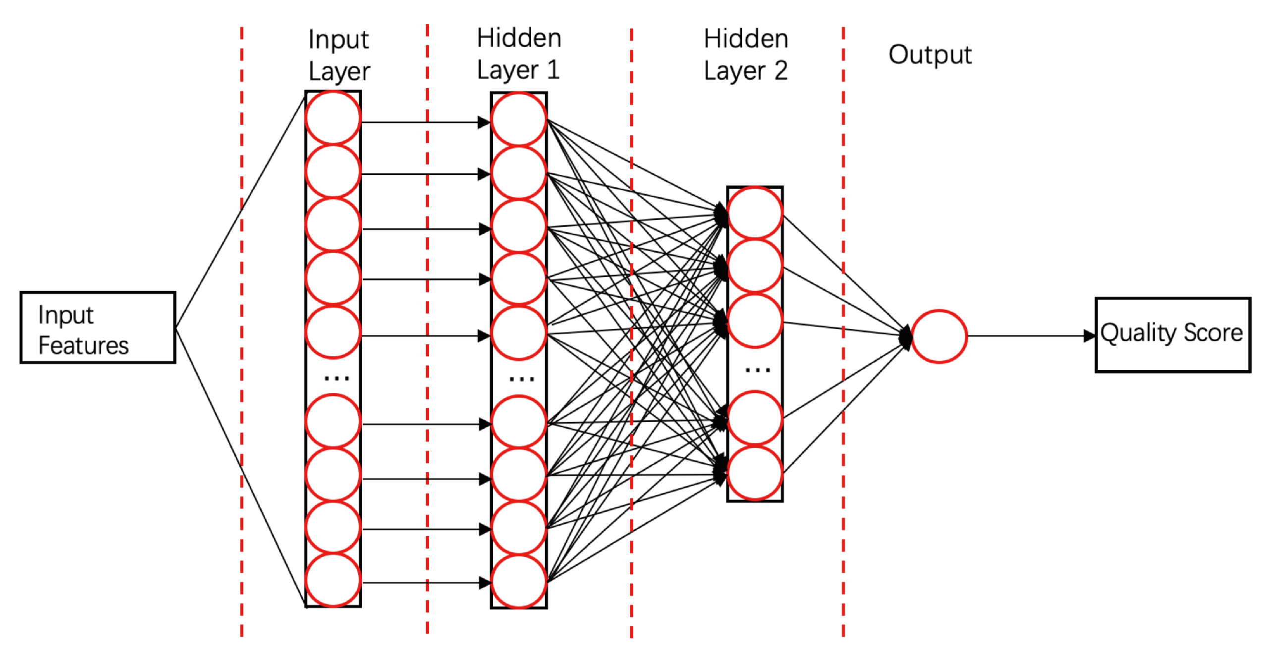
- ProQ3D [58]ProQ3D includes all the features of ProQ3, but replaces the SVM model in ProQ3 with a multi-layer perceptron NN model containing two hidden layers. The first hidden layer contains 600 neural cells, and the second layer contains 200 neural cells and a rectified linear-unit activation function (as shown in Figure 4). Table A1 compares the performances of ProQ3D and its predecessors (ProQ, ProQ2, ProQ2D, and ProQ3) on the CASP11 data source. ProQ3D outperformed the other models in terms of Pearson correlation (0.90 for global quality, 0.77 for local quality), the area under the curve measure (AUC = 0.91), and GDT_TS score loss (0.006). As ProQ3D takes the same input features as ProQ3, the improvement is wholly and remarkably attributable to the improved learning model in ProQ3D. In the recent CASP13, the final version of ProQ3D outperformed ProQ3 in almost all measures [20]. It also performed as the second best single-model method in the “top 1 loss” analysis (ranking top model) of global quality assessment; this indicates that ProQ3D has great potential for global quality prediction.
- ModFOLD is a series of EMA methods (the first version was pioneered by McGuffin [95] in 2008). ModFOLD6 and ModFOLD7 are the latest two generations, which were proposed for CASP12 and CASP13, respectively. Both methods achieved the best performance in the QA category of CASP. ModFOLD6 & 7 have similar working pipelines; different pure-single models and quasi-single models independently assess the features of a protein model and generate their own local quality scores. These local quality scores are considered as features and fed into an NN that derives the final predicted local score. Finally, the per-residue scores of the different methods are averaged to give the predicted global score. ModFOLD6 adopted ProQ2 [33], contact distance agreement (CDA) and secondary structure agreement (SSA) as pure-single methods and disorder B-factor agreement (DBA) [34,96], ModFOLD5 (MF5s) [97], and ModFOLDclustQ (MFcQs) [24] as quasi-single methods. ModFOLD6 was tested on CASP12 and part of the CAMEO set. Table A2 compares the performances of ModFOLD6 and other methods on CAMEO. The AUC score of ModFOLD6 (0.8748) far exceeded those of the other EMA methods (ProQ2, Verify3d, Dfire), and slightly surpasses that of ModFOLD4. This result demonstrates that a hybrid method has potential as a high-performing EMA method. In ModFOLD7, in order to improve the local quality prediction accuracy and the consistency of single model ranking and scoring, it adopts ten pure-single and quasi-single methods, including CDA, SSA, ProQ, ProQ2D, ProQ3D, VoroMQA, DBA, MF5s, MFcQs, and ResQ7 [98]. In CASP13, ModFOLD7 is one of the best methods for global quality assessment [31]. It provides two working versions of the method. ModFOLD7_rank is the best in ranking top models (assessed by the top one loss on GDT_TS and LDDT), and ModFOLD7_cor is good at reflecting observed accuracy scores or estimating the absolute error (based on the Z-score of GDT-TS differences and LDDT differences) [20].
- Proposed by Hou et al., MULTICOM is a protein structure prediction method. Two sub-models, MULTICOM_cluster and MULTICOM_construct, had outstanding performances in the QA category of CASP13. They were the best methods in both the “top 1 loss” assessment (the top one losses on GDT_TS and LDDT were 5.2 and 3.9, respectively) and “absolute accuracy estimation” (based on Z-score of GDT-TS differences and LDDT differences) [31]. Similar to ModFOLD, MULTICOM uses a hybrid approach to assess the global quality of a protein model. Prediction results from 12 different QA methods (9 single-models, 3 multi-models) and 1 protein contact predictor (DNCON2 [99]) are taken as input features for 10 pretrained deep neural networks. Each of these DNNs generates one quality score for the given target model. For MULTICOM_construct, the final quality score is simply the mean of 10 quality scores predicted by DNNs. However, for MULTICOM_cluster, the combination of 13 primary prediction results and 10 DNN prediction results will be further put into another DNN for final quality score prediction. Their experiment showed that the residue-residue contact feature greatly improves the performance of the method, even though its impact varies depending on the accuracy of contact prediction. The success of MULTICOM has brought the residue-residue contact feature to the spotlight, such that it can consistently improve the performance of EMA methods adopting this or related features [20]. New advances in contact prediction based on DL and co-evolutionary analysis techniques may further improve EMA performance [40].
3.3. Convolutional Neural Networks
- ProQ4 [21]ProQ4 inputs various protein structural features such as the dihedral angles and , the protein secondary structure, the hydrogen bond energies, and statistical features of the sequence. The method has a multi-stream structure and trains each stream separately, which is feasible for transfer learning of the protein-structure quality assessment. ProQ4 was trained on CASP9 and CASP10 and tested on CASP11, CAMEO, and PISCES. On the CASP11 data source, ProQ4 delivered a poorer local performance than ProQ3D, but a significantly higher global performance. The local and global performances of ProQ4 and ProQ3D are given in Table A3 and Table A4, respectively. This method also proves the importance of the protein structure information in EMA. In addition, one of the main reasons for designing ProQ4 is to improve its target ranking ability. The result of CASP13 showed that ProQ4 successfully improved its target ranking over ProQ3D although its overall performance (GDT_TS, TM, CAD, and lDDT) was not better [20].
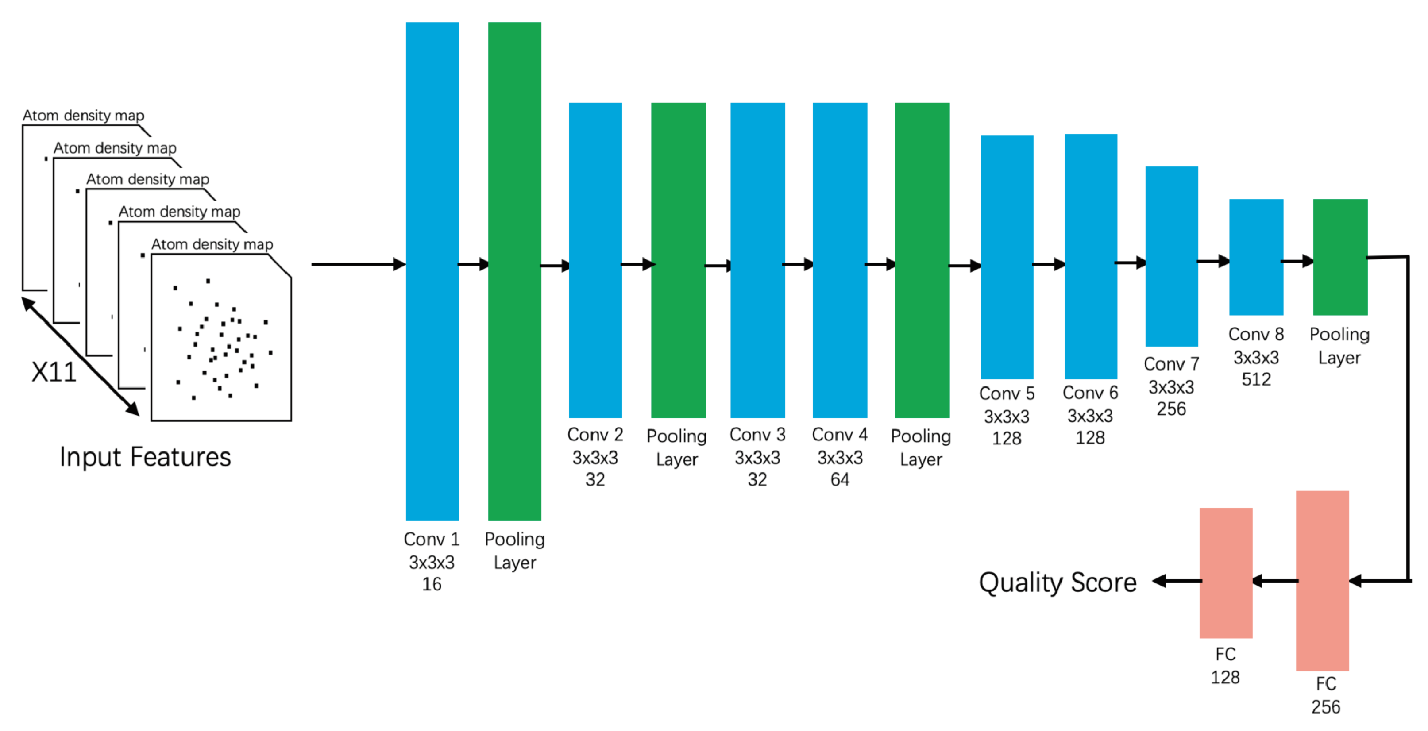
- 3DCNN_MQA [91]This state-of-the-art method inputs three-dimensional atom density maps of the predicted protein and analyzes 11 types of atoms. The success of this method proves the feasibility of inputting low-level raw data. During the training process, 3DCNN uniquely calculates the loss of the GDT_TS score rather than the GDT_TS score [91]. This method was trained on CASP7–CASP10 and validated on CASP11, CASP12, and CAMEO. The losses, Pearson’s correlations, Spearman’s correlations, and Kendall’s correlations of 3DCNN on CASP11 were 0.064, 0.535, 0.425, and 0.325 respectively in Stage 1 and 0.064, 0.421, 0.409, and 0.288 respectively in Stage 2 (Table A5). Unlike highly feature-engineered methods such as ProQ3D [58] and ProQ2D, this method uses simple atomic features, but is able to achieve moderate performance on CASP11.
- The original 3DCNN has two limitations, the resolution problem caused by different protein sizes and the orientation problem caused by different protein positions in 3D space. In order to solve these problems, Pages et al. developed Ornate [92] (oriented routed neural network with automatic typing), which is a single-model EMA method. Instead of using 3D density maps in the protein level, it breaks the density maps into residue level and aligns each map by the backbone topology, then these features are used as input data for a deep convolutional neural network. The local score is generated first, and the average of all local scores is taken as the final global score. Evaluation results on CASP11 and CASP12 showed that Ornate was competitive with most state-of-the-art single-model EMA methods. However, complex input features required by Ornate demand more processing time and computational resources during the learning process, which might be an obstacle for further improvement. Inspired by the original 3DCNN_MQA [91] and Ornate [92], Sato et al. proposed a new 3DCNN-based MQA method. There, the simplified atom categories and network topologies were used for predictive modeling so that the model could be more easily trained. The performances of 3DCNN_MQA (Sato) surpassed 3DCNN_MQA (Derevyanko) on the CASP11, CASP12, and 3DRobot datasets. The best performance of 3DCNN_MQA (Sato) was achieved in Stage 2 of CASP11; it outperformed all other state-of-the-art EMA methods on Spearman’s and Pearson’s correlation coefficients.
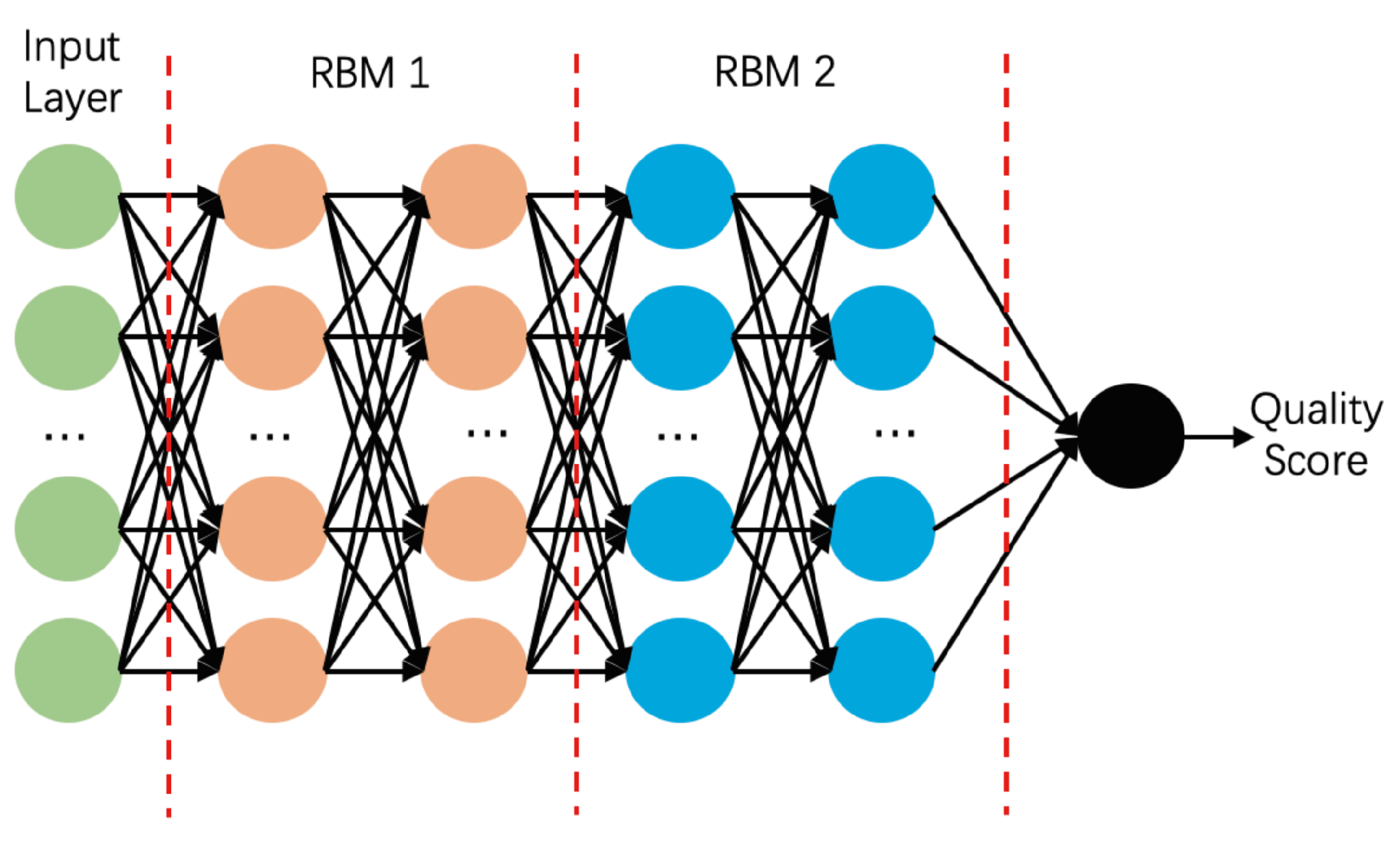
3.4. Deep Belief Network
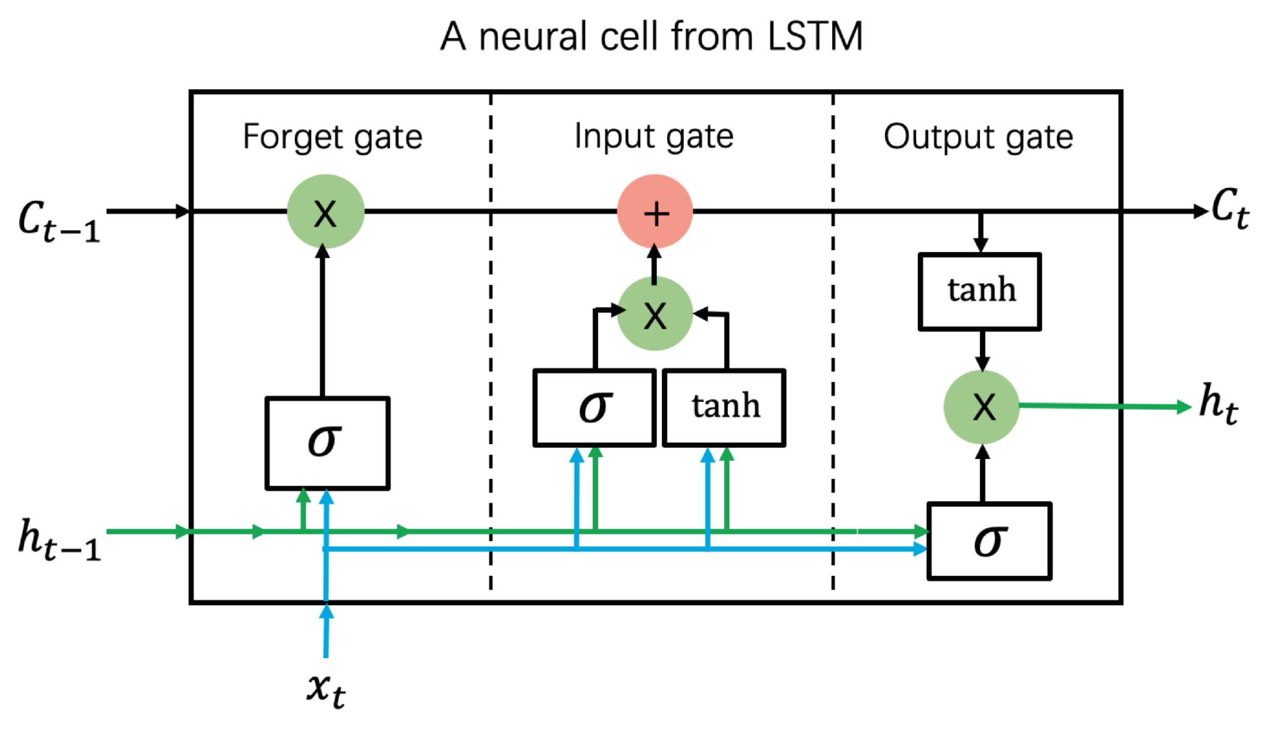
3.5. Long Short-Term Memory
3.6. Ensemble Learning
3.7. Bayesian Learning
4. Summary and Future Perspectives
Author Contributions
Funding
Conflicts of Interest
Appendix A. The Performances of ML-based EMA Methods

| Model | CC-Glob | CC-Target | CC-Loc | CC-Model | AUC | GDT TS Loss |
|---|---|---|---|---|---|---|
| ProQ | 0.60 | 0.44 | 0.50 | 0.39 | 0.78 | 0.06 |
| ProQ2 | 0.81 | 0.65 | 0.69 | 0.47 | 0.83 | 0.06 |
| ProQ2D | 0.85 | 0.68 | 0.72 | 0.49 | 0.89 | 0.05 |
| ProQ3 | 0.85 | 0.65 | 0.73 | 0.51 | 0.89 | 0.06 |
| ProQ3D | 0.90 | 0.71 | 0.77 | 0.54 | 0.91 | 0.06 |
| Model | AUC | StdErr | AUC 0–0.1 | AUC 0–0.1 Rescaled |
|---|---|---|---|---|
| ModFOLD6 | 0.8748 | 0.00096 | 0.0508 | 0.5081 |
| ModFOLD4 | 0.8638 | 0.00099 | 0.0467 | 0.4669 |
| ProQ2 | 0.8374 | 0.00107 | 0.0428 | 0.4283 |
| Verify3d | 0.7020 | 0.00134 | 0.0208 | 0.2081 |
| Dfire v1.1 | 0.6606 | 0.00138 | 0.0168 | 0.1675 |
| Method | R-Local | RMSE Local | local R-per Model |
|---|---|---|---|
| ProQ3D | 0.84 | 0.125 | 0.61 |
| ProQ4 | 0.77 | 0.147 | 0.56 |
| Method | R-Global | RMSE Global | R-per Target | First Rank Loss |
|---|---|---|---|---|
| ProQ3D | 0.90 | 0.080 | 0.82 | 0.040 |
| ProQ4 | 0.91 | 0.085 | 0.90 | 0.022 |
| Method | Loss 1 | Pearson | Spearman | Kendall |
|---|---|---|---|---|
| Stage 1 | ||||
| ProQ3D | 0.046 | 0.755 | 0.673 | 0.529 |
| ProQ2D | 0.064 | 0.729 | 0.604 | 0.468 |
| 3DCNN_MQA | 0.064 | 0.535 | 0.425 | 0.325 |
| VoroMQA | 0.087 | 0.637 | 0.521 | 0.394 |
| RWplus | 0.122 | 0.512 | 0.402 | 0.303 |
| Stage 2 | ||||
| VoroMQA | 0.063 | 0.457 | 0.449 | 0.321 |
| 3DCNN_MQA | 0.064 | 0.421 | 0.409 | 0.288 |
| ProQ3D | 0.066 | 0.452 | 0.433 | 0.307 |
| ProQ2D | 0.072 | 0.437 | 0.422 | 0.299 |
| RWplus | 0.089 | 0.206 | 0.248 | 0.176 |
| Method | Corr. on Stage 1 | Loss on Stage 1 | Corr. on Stage 2 | Loss on Stage 2 |
|---|---|---|---|---|
| DeepQA | 0.64 | 0.09 | 0.42 | 0.06 |
| ProQ2 | 0.64 | 0.09 | 0.37 | 0.06 |
| Qprob | 0.63 | 0.10 | 0.38 | 0.07 |
| Wang_SVM | 0.66 | 0.11 | 0.36 | 0.09 |
| Wang_deep_2 | 0.63 | 0.12 | 0.31 | 0.09 |
| Wang_deep_1 | 0.61 | 0.13 | 0.30 | 0.09 |
| Wang_deep_3 | 0.63 | 0.12 | 0.30 | 0.09 |
| RFMQA | 0.54 | 0.12 | 0.29 | 0.08 |
| ProQ3 | 0.65 | 0.07 | 0.38 | 0.06 |
| Method | Corr. on Stage 1 | Loss on Stage 1 | Corr. on Stage 2 | Loss on Stage 2 |
|---|---|---|---|---|
| AngularQA | 0.545 | 0.116 | 0.393 | 0.128 |
| ProQ3 | 0.638 | 0.048 | 0.616 | 0.068 |
| DeepQA | 0.654 | 0.078 | 0.578 | 0.100 |
| Wang1 | 0.462 | 0.170 | 0.256 | 0.144 |
| QMEAN | 0.342 | 0.174 | 0.292 | 0.125 |
References
- Jacobson, M.; Sali, A. Comparative protein structure modeling and its applications to drug discovery. Annu. Rep. Med. Chem. 2004, 39, 259–274. [Google Scholar]
- Gawehn, E.; Hiss, J.; Schneider, G. Deep Learning in Drug Discovery. Mol. Inform. 2016, 35, 3–14. [Google Scholar] [CrossRef] [PubMed]
- Eswar, N.; Webb, B.; Marti-Renom, M.A.; Madhusudhan, M.; Eramian, D.; Shen, M.Y.; Pieper, U.; Sali, A. Comparative protein structure modeling using Modeller. Curr. Protoc. Bioinforma. 2006, 15, 5–6. [Google Scholar] [CrossRef] [PubMed]
- Waterhouse, A.; Bertoni, M.; Bienert, S.; Studer, G.; Tauriello, G.; Gumienny, R.; Heer, F.T.; de Beer, T.A.P.; Rempfer, C.; Bordoli, L.; et al. SWISS-MODEL: Homology modeling of protein structures and complexes. Nucleic Acids Res. 2018, 46, W296–W303. [Google Scholar] [CrossRef]
- Rohl, C.A.; Strauss, C.E.; Misura, K.M.; Baker, D. Protein structure prediction using Rosetta. In Methods in Enzymology; Elsevier: Amsterdam, The Netherlands, 2004; Volume 383, pp. 66–93. [Google Scholar]
- Simons, K.T.; Bonneau, R.; Ruczinski, I.; Baker, D. Ab initio protein structure prediction of CASP III targets using ROSETTA. Proteins Struct. Funct. Bioinforma. 1999, 37, 171–176. [Google Scholar] [CrossRef]
- Zhang, Y. I-TASSER server for protein 3D structure prediction. BMC Bioinforma. 2008, 9, 40. [Google Scholar] [CrossRef]
- Wang, C.; Zhang, H.; Zheng, W.M.; Xu, D.; Zhu, J.; Wang, B.; Ning, K.; Sun, S.; Li, S.C.; Bu, D. FALCON@ home: A high-throughput protein structure prediction server based on remote homologue recognition. Bioinformatics 2016, 32, 462–464. [Google Scholar] [CrossRef]
- Xu, J.; Li, M.; Kim, D.; Xu, Y. RAPTOR: Optimal protein threading by linear programming. J. Bioinforma. Comput. Biol. 2003, 1, 95–117. [Google Scholar] [CrossRef]
- Källberg, M.; Wang, H.; Wang, S.; Peng, J.; Wang, Z.; Lu, H.; Xu, J. Template-based protein structure modeling using the RaptorX web server. Nat. Protoc. 2012, 7, 1511–1522. [Google Scholar] [CrossRef]
- McGuffin, L.J.; Adiyaman, R.; Maghrabi, A.H.; Shuid, A.N.; Brackenridge, D.A.; Nealon, J.O.; Philomina, L.S. IntFOLD: An integrated web resource for high performance protein structure and function prediction. Nucleic Acids Res. 2019, 47, W408–W413. [Google Scholar] [CrossRef]
- Kuhlman, B.; Bradley, P. Advances in protein structure prediction and design. Nat. Rev. Mol. Cell Biol. 2019, 20, 681–697. [Google Scholar] [CrossRef]
- Kryshtafovych, A.; Schwede, T.; Topf, M.; Fidelis, K.; Moult, J. Critical assessment of methods of protein structure prediction (CASP)—Round XIII. Proteins Struct. Funct. Bioinforma. 2019, 87, 1011–1020. [Google Scholar] [CrossRef]
- Hessler, G.; Baringhaus, K.H. Artificial intelligence in drug design. Molecules 2018, 23, 2520. [Google Scholar] [CrossRef]
- Zhao, F.; Zheng, L.; Goncearenco, A.; Panchenko, A.R.; Li, M. Computational approaches to prioritize cancer driver missense mutations. Int. J. Mol. Sci. 2018, 19, 2113. [Google Scholar] [CrossRef]
- Chen, R.; Liu, X.; Jin, S.; Lin, J.; Liu, J. Machine learning for drug-target interaction prediction. Molecules 2018, 23, 2208. [Google Scholar] [CrossRef]
- Wu, Y.; Wang, G. Machine learning based toxicity prediction: From chemical structural description to transcriptome analysis. Int. J. Mol. Sci. 2018, 19, 2358. [Google Scholar] [CrossRef]
- AlQuraishi, M. ProteinNet: A standardized data set for machine learning of protein structure. BMC Bioinforma. 2019, 20, 311. [Google Scholar] [CrossRef]
- Kryshtafovych, A.; Monastyrskyy, B.; Fidelis, K.; Schwede, T.; Tramontano, A. Assessment of model accuracy estimations in CASP12. Proteins Struct. Funct. Bioinforma. 2018, 86, 345–360. [Google Scholar] [CrossRef] [PubMed]
- Cheng, J.; Choe, M.H.; Elofsson, A.; Han, K.S.; Hou, J.; Maghrabi, A.H.; McGuffin, L.J.; Menéndez-Hurtado, D.; Olechnovič, K.; Schwede, T.; et al. Estimation of model accuracy in CASP13. Proteins Struct. Funct. Bioinforma. 2019, 87, 1361–1377. [Google Scholar] [CrossRef] [PubMed]
- Hurtado, D.M.; Uziela, K.; Elofsson, A. Deep transfer learning in the assessment of the quality of protein models. arXiv 2018, arXiv:1804.06281. [Google Scholar]
- Uziela, K.; Shu, N.; Wallner, B.; Elofsson, A. ProQ3: Improved model quality assessments using Rosetta energy terms. Sci. Rep. 2016, 6, 33509. [Google Scholar] [CrossRef]
- Manavalan, B.; Lee, J. SVMQA: Support–vector-machine-based protein single-model quality assessment. Bioinformatics 2017, 33, 2496–2503. [Google Scholar] [CrossRef]
- McGuffin, L.J.; Roche, D.B. Rapid model quality assessment for protein structure predictions using the comparison of multiple models without structural alignments. Bioinformatics 2010, 26, 182–188. [Google Scholar] [CrossRef]
- Wallner, B.; Elofsson, A. Identification of correct regions in protein models using structural, alignment, and consensus information. Protein Sci. 2006, 15, 900–913. [Google Scholar] [CrossRef]
- Cao, R.; Bhattacharya, D.; Adhikari, B.; Li, J.; Cheng, J. Large-scale model quality assessment for improving protein tertiary structure prediction. Bioinformatics 2015, 31, i116–i123. [Google Scholar] [CrossRef]
- Cozzetto, D.; Kryshtafovych, A.; Tramontano, A. Evaluation of CASP8 model quality predictions. Proteins Struct. Funct. Bioinforma. 2009, 77, 157–166. [Google Scholar] [CrossRef] [PubMed]
- Kryshtafovych, A.; Fidelis, K.; Tramontano, A. Evaluation of model quality predictions in CASP9. Proteins Struct. Funct. Bioinforma. 2011, 79, 91–106. [Google Scholar] [CrossRef] [PubMed]
- Kryshtafovych, A.; Barbato, A.; Fidelis, K.; Monastyrskyy, B.; Schwede, T.; Tramontano, A. Assessment of the assessment: Evaluation of the model quality estimates in CASP10. Proteins Struct. Funct. Bioinforma. 2014, 82, 112–126. [Google Scholar] [CrossRef] [PubMed]
- Kryshtafovych, A.; Barbato, A.; Monastyrskyy, B.; Fidelis, K.; Schwede, T.; Tramontano, A. Methods of model accuracy estimation can help selecting the best models from decoy sets: Assessment of model accuracy estimations in CASP 11. Proteins Struct. Funct. Bioinforma. 2016, 84, 349–369. [Google Scholar] [CrossRef] [PubMed]
- Won, J.; Baek, M.; Monastyrskyy, B.; Kryshtafovych, A.; Seok, C. Assessment of protein model structure accuracy estimation in CASP13: Challenges in the era of deep learning. Proteins Struct. Funct. Bioinforma. 2019, 87, 1351–1360. [Google Scholar] [CrossRef]
- Wang, W.; Wang, J.; Xu, D.; Shang, Y. Two new heuristic methods for protein model quality assessment. IEEE/ACM Trans. Comput. Biol. Bioinforma. 2018. [Google Scholar] [CrossRef] [PubMed]
- Ray, A.; Lindahl, E.; Wallner, B. Improved model quality assessment using ProQ2. BMC Bioinforma. 2012, 13, 224. [Google Scholar] [CrossRef] [PubMed]
- Maghrabi, A.H.; McGuffin, L.J. ModFOLD6: An accurate web server for the global and local quality estimation of 3D protein models. Nucleic Acids Res. 2017, 45, W416–W421. [Google Scholar] [CrossRef]
- Cao, R.; Cheng, J. Protein single-model quality assessment by feature-based probability density functions. Sci. Rep. 2016, 6, 23990. [Google Scholar] [CrossRef] [PubMed]
- Portugal, I.; Alencar, P.; Cowan, D. The use of machine learning algorithms in recommender systems: A systematic review. Expert Syst. Appl. 2018, 97, 205–227. [Google Scholar] [CrossRef]
- Kotsiantis, S.B.; Zaharakis, I.; Pintelas, P. Supervised machine learning: A review of classification techniques. Emerg. Artif. Intell. Appl. Comput. Eng. 2007, 160, 3–24. [Google Scholar]
- Kandathil, S.M.; Greener, J.G.; Jones, D.T. Recent developments in deep learning applied to protein structure prediction. Proteins Struct. Funct. Bioinforma. 2019, 87, 1179–1189. [Google Scholar] [CrossRef]
- Mirabello, C.; Wallner, B. rawMSA: End-to-end Deep Learning using raw Multiple Sequence Alignments. PLoS ONE 2019, 14, e0220182. [Google Scholar] [CrossRef]
- Xu, J. Distance-based protein folding powered by deep learning. Proc. Natl. Acad. Sci. USA 2019, 116, 16856–16865. [Google Scholar] [CrossRef]
- Essen, L.O. Structural Bioinformatics. Edited by Philip E. Bourne and Helge Weissig. Angew. Chem. Int. Ed. 2003, 42, 4993. [Google Scholar] [CrossRef]
- Schlick, T. Molecular Modeling and Simulation: An Interdisciplinary Guide; Springer: New York, NY, USA, 2010; Volume 21. [Google Scholar]
- Kihara, D. (Ed.) Protein Structure Prediction; Humana Press: New York, NY, USA, 2014. [Google Scholar]
- Lee, J.; Freddolino, P.L.; Zhang, Y. Ab initio protein structure prediction. In From Protein Structure to Function With Bioinformatics; Springer: Dordrecht, The Netherlands, 2017; pp. 3–35. [Google Scholar]
- De Oliveira, S.; Deane, C. Co-evolution techniques are reshaping the way we do structural bioinformatics. F1000Research 2017, 6, 1224. [Google Scholar] [CrossRef] [PubMed]
- Marks, D.S.; Colwell, L.J.; Sheridan, R.; Hopf, T.A.; Pagnani, A.; Zecchina, R.; Sander, C. Protein 3D structure computed from evolutionary sequence variation. PLoS ONE 2011, 6, e28766. [Google Scholar] [CrossRef] [PubMed]
- Marks, D.S.; Hopf, T.A.; Sander, C. Protein structure prediction from sequence variation. Nat. Biotechnol. 2012, 30, 1072. [Google Scholar] [CrossRef]
- Morcos, F.; Pagnani, A.; Lunt, B.; Bertolino, A.; Marks, D.S.; Sander, C.; Zecchina, R.; Onuchic, J.N.; Hwa, T.; Weigt, M. Direct-coupling analysis of residue coevolution captures native contacts across many protein families. Proc. Natl. Acad. Sci. USA 2011, 108, E1293–E1301. [Google Scholar] [CrossRef] [PubMed]
- De Juan, D.; Pazos, F.; Valencia, A. Emerging methods in protein co-evolution. Nat. Rev. Genet. 2013, 14, 249–261. [Google Scholar] [CrossRef]
- Senior, A.W.; Evans, R.; Jumper, J.; Kirkpatrick, J.; Sifre, L.; Green, T.; Qin, C.; Žídek, A.; Nelson, A.W.; Bridgland, A.; et al. Improved protein structure prediction using potentials from deep learning. Nature 2020, 577, 706–710. [Google Scholar] [CrossRef]
- Senior, A.W.; Evans, R.; Jumper, J.; Kirkpatrick, J.; Sifre, L.; Green, T.; Qin, C.; Žídek, A.; Nelson, A.W.; Bridgland, A.; et al. Protein structure prediction using multiple deep neural networks in the 13th Critical Assessment of Protein Structure Prediction (CASP13). Proteins Struct. Funct. Bioinforma. 2019, 87, 1141–1148. [Google Scholar] [CrossRef]
- Hou, J.; Wu, T.; Cao, R.; Cheng, J. Protein tertiary structure modeling driven by deep learning and contact distance prediction in CASP13. Proteins Struct. Funct. Bioinforma. 2019, 87, 1165–1178. [Google Scholar] [CrossRef]
- Moult, J.; Fidelis, K.; Kryshtafovych, A.; Schwede, T.; Tramontano, A. Critical assessment of methods of protein structure prediction (CASP)—Round x. Proteins Struct. Funct. Bioinforma. 2014, 82, 1–6. [Google Scholar] [CrossRef]
- Lima, E.C.; Custódio, F.L.; Rocha, G.K.; Dardenne, L.E. Estimating Protein Structure Prediction Models Quality Using Convolutional Neural Networks. In Proceedings of the 2018 International Joint Conference on Neural Networks (IJCNN), Rio de Janeiro, Brazil, 8–13 July 2018; pp. 1–6. [Google Scholar]
- Cozzetto, D.; Kryshtafovych, A.; Ceriani, M.; Tramontano, A. Assessment of predictions in the model quality assessment category. Proteins Struct. Funct. Bioinforma. 2007, 69, 175–183. [Google Scholar] [CrossRef]
- Studer, G.; Rempfer, C.; Waterhouse, A.M.; Gumienny, R.; Haas, J.; Schwede, T. QMEANDisCo—Distance constraints applied on model quality estimation. Bioinformatics 2020, 36, 1765–1771. [Google Scholar] [CrossRef] [PubMed]
- 13th Community Wide Experiment on the Critical Assessment of Techniques for Protein Structure Prediction—Abstracts. Available online: http://predictioncenter.org/casp13/doc/CASP13_Abstracts.pdf (accessed on 31 March 2020).
- Uziela, K.; Menéndez Hurtado, D.; Shu, N.; Wallner, B.; Elofsson, A. ProQ3D: Improved model quality assessments using deep learning. Bioinformatics 2017, 33, 1578–1580. [Google Scholar] [CrossRef] [PubMed]
- Olechnovič, K.; Venclovas, Č. VoroMQA: Assessment of protein structure quality using interatomic contact areas. Proteins Struct. Funct. Bioinforma. 2017, 85, 1131–1145. [Google Scholar] [CrossRef] [PubMed]
- Antczak, P.L.M.; Ratajczak, T.; Lukasiak, P.; Blazewicz, J. SphereGrinder-reference structure-based tool for quality assessment of protein structural models. In Proceedings of the 2015 IEEE International Conference on Bioinformatics and Biomedicine (BIBM), Washington, DC, USA, 9–12 November 2015; pp. 665–668. [Google Scholar]
- Zemla, A. LGA: A method for finding 3D similarities in protein structures. Nucleic Acids Res. 2003, 31, 3370–3374. [Google Scholar] [CrossRef]
- Zemla, A.; Venclovas, Č.; Moult, J.; Fidelis, K. Processing and evaluation of predictions in CASP4. Proteins Struct. Funct. Bioinforma. 2001, 45, 13–21. [Google Scholar] [CrossRef] [PubMed]
- Olechnovič, K.; Kulberkytė, E.; Venclovas, Č. CAD-score: A new contact area difference-based function for evaluation of protein structural models. Proteins Struct. Funct. Bioinforma. 2013, 81, 149–162. [Google Scholar] [CrossRef]
- Nguyen, S.P.; Shang, Y.; Xu, D. DL-PRO: A novel deep learning method for protein model quality assessment. In Proceedings of the 2014 International Joint Conference on Neural Networks (IJCNN), Beijing, China, 6–11 July 2014; pp. 2071–2078. [Google Scholar]
- Mariani, V.; Biasini, M.; Barbato, A.; Schwede, T. lDDT: A local superposition-free score for comparing protein structures and models using distance difference tests. Bioinformatics 2013, 29, 2722–2728. [Google Scholar] [CrossRef]
- Zhang, Y.; Skolnick, J. Scoring function for automated assessment of protein structure template quality. Proteins Struct. Funct. Bioinforma. 2004, 57, 702–710. [Google Scholar] [CrossRef]
- Wang, S.; Ma, J.; Peng, J.; Xu, J. Protein structure alignment beyond spatial proximity. Sci. Rep. 2013, 3, 1448. [Google Scholar] [CrossRef]
- Local Distance Difference Test—Swiss Model. Available online: https://swissmodel.expasy.org/lddt/help/ (accessed on 14 April 2019).
- Benesty, J.; Chen, J.; Huang, Y.; Cohen, I. Pearson correlation coefficient. In Noise Reduction in Speech Processing; Springer: Berlin/Heidelberg, Germany, 2009; pp. 1–4. [Google Scholar]
- Hauke, J.; Kossowski, T. Comparison of values of Pearson’s and Spearman’s correlation coefficients on the same sets of data. Quaest. Geogr. 2011, 30, 87–93. [Google Scholar] [CrossRef]
- Mukaka, M.M. A guide to appropriate use of correlation coefficient in medical research. Malawi Med J. 2012, 24, 69–71. [Google Scholar] [PubMed]
- Abdi, H. The Kendall rank correlation coefficient. In Encyclopedia of Measurement and Statistics; Sage: Thousand Oaks, CA, USA, 2007; pp. 508–510. [Google Scholar]
- Wang, Z.; Tegge, A.N.; Cheng, J. Evaluating the absolute quality of a single protein model using structural features and support vector machines. Proteins Struct. Funct. Bioinforma. 2009, 75, 638–647. [Google Scholar] [CrossRef] [PubMed]
- Cao, R.; Bhattacharya, D.; Hou, J.; Cheng, J. DeepQA: Improving the estimation of single protein model quality with deep belief networks. BMC Bioinforma. 2016, 17, 495. [Google Scholar] [CrossRef] [PubMed]
- Cheng, J.; Randall, A.Z.; Sweredoski, M.J.; Baldi, P. SCRATCH: A protein structure and structural feature prediction server. Nucleic Acids Res. 2005, 33, W72–W76. [Google Scholar] [CrossRef]
- Jones, S.; Daley, D.T.; Luscombe, N.M.; Berman, H.M.; Thornton, J.M. Protein–RNA interactions: A structural analysis. Nucleic Acids Res. 2001, 29, 943–954. [Google Scholar] [CrossRef]
- NACCESS-ComputerProgram. 1993. Available online: http://wolf.bms.umist.ac.uk/naccess/ (accessed on 14 April 2019).
- Conover, M.; Staples, M.; Si, D.; Sun, M.; Cao, R. AngularQA: Protein model quality assessment with LSTM networks. Comput. Math. Biophys. 2019, 7, 1–9. [Google Scholar] [CrossRef]
- Liu, T.; Wang, Y.; Eickholt, J.; Wang, Z. Benchmarking deep networks for predicting residue-specific quality of individual protein models in CASP11. Sci. Rep. 2016, 6, 19301. [Google Scholar] [CrossRef]
- Manavalan, B.; Lee, J.; Lee, J. Random forest-based protein model quality assessment (RFMQA) using structural features and potential energy terms. PLoS ONE 2014, 9, e106542. [Google Scholar] [CrossRef]
- Yang, Y.; Zhou, Y. Specific interactions for ab initio folding of protein terminal regions with secondary structures. Proteins Struct. Funct. Bioinforma. 2008, 72, 793–803. [Google Scholar] [CrossRef]
- Zhang, J.; Zhang, Y. A novel side-chain orientation dependent potential derived from random-walk reference state for protein fold selection and structure prediction. PLoS ONE 2010, 5, e15386. [Google Scholar] [CrossRef]
- Zhou, H.; Skolnick, J. GOAP: A generalized orientation-dependent, all-atom statistical potential for protein structure prediction. Biophys. J. 2011, 101, 2043–2052. [Google Scholar] [CrossRef] [PubMed]
- Mirzaei, S.; Sidi, T.; Keasar, C.; Crivelli, S. Purely structural protein scoring functions using support vector machine and ensemble learning. IEEE/ACM Trans. Comput. Biol. Bioinforma. 2016, 16, 1515–1523. [Google Scholar] [CrossRef] [PubMed]
- Cao, R.; Adhikari, B.; Bhattacharya, D.; Sun, M.; Hou, J.; Cheng, J. QAcon: Single model quality assessment using protein structural and contact information with machine learning techniques. Bioinformatics 2017, 33, 586–588. [Google Scholar] [CrossRef]
- Wang, G.; Dunbrack, R.L., Jr. PISCES: A protein sequence culling server. Bioinformatics 2003, 19, 1589–1591. [Google Scholar] [CrossRef] [PubMed]
- Haas, J.; Roth, S.; Arnold, K.; Kiefer, F.; Schmidt, T.; Bordoli, L.; Schwede, T. The Protein Model Portal—A comprehensive resource for protein structure and model information. Database 2013, 2013, bat031. [Google Scholar] [CrossRef]
- Deng, H.; Jia, Y.; Zhang, Y. 3DRobot: Automated generation of diverse and well-packed protein structure decoys. Bioinformatics 2016, 32, 378–387. [Google Scholar] [CrossRef] [PubMed]
- Wu, S.; Skolnick, J.; Zhang, Y. Ab initio modeling of small proteins by iterative TASSER simulations. BMC Biol. 2007, 5, 17. [Google Scholar] [CrossRef]
- CAMEO Continuously Evaluate the Accuracy and Reliability of Predictions. Available online: https://www.cameo3d.org/ (accessed on 14 April 2019).
- Derevyanko, G.; Grudinin, S.; Bengio, Y.; Lamoureux, G. Deep convolutional networks for quality assessment of protein folds. Bioinformatics 2018, 34, 4046–4053. [Google Scholar] [CrossRef]
- Pagès, G.; Charmettant, B.; Grudinin, S. Protein model quality assessment using 3D oriented convolutional neural networks. Bioinformatics 2019, 35, 3313–3319. [Google Scholar] [CrossRef]
- Sato, R.; Ishida, T. Protein model accuracy estimation based on local structure quality assessment using 3D convolutional neural network. PLoS ONE 2019, 14, e0221347. [Google Scholar] [CrossRef]
- Cortes, C.; Vapnik, V. Support-vector networks. Mach. Learn. 1995, 20, 273–297. [Google Scholar] [CrossRef]
- McGuffin, L.J. The ModFOLD server for the quality assessment of protein structural models. Bioinformatics 2008, 24, 586–587. [Google Scholar] [CrossRef] [PubMed]
- Jones, D.T.; Cozzetto, D. DISOPRED3: Precise disordered region predictions with annotated protein-binding activity. Bioinformatics 2015, 31, 857–863. [Google Scholar] [CrossRef] [PubMed]
- McGuffin, L.J.; Buenavista, M.T.; Roche, D.B. The ModFOLD4 server for the quality assessment of 3D protein models. Nucleic Acids Res. 2013, 41, W368–W372. [Google Scholar] [CrossRef] [PubMed]
- Yang, J.; Wang, Y.; Zhang, Y. ResQ: An approach to unified estimation of B-factor and residue-specific error in protein structure prediction. J. Mol. Biol. 2016, 428, 693–701. [Google Scholar] [CrossRef] [PubMed]
- Adhikari, B.; Hou, J.; Cheng, J. DNCON2: Improved protein contact prediction using two-level deep convolutional neural networks. Bioinformatics 2018, 34, 1466–1472. [Google Scholar] [CrossRef]
- Hinton, G.E.; Osindero, S.; Teh, Y.W. A fast learning algorithm for deep belief nets. Neural Comput. 2006, 18, 1527–1554. [Google Scholar] [CrossRef]
- Le Roux, N.; Bengio, Y. Representational power of restricted Boltzmann machines and deep belief networks. Neural Comput. 2008, 20, 1631–1649. [Google Scholar] [CrossRef]
- Hinton, G.E. Deep belief networks. Scholarpedia 2009, 4, 5947. [Google Scholar] [CrossRef]
- Mohamed, A.R.; Dahl, G.E.; Hinton, G. Acoustic modeling using deep belief networks. IEEE Trans. Audio Speech Lang. Process. 2011, 20, 14–22. [Google Scholar] [CrossRef]
- Nawi, N.M.; Ransing, M.R.; Ransing, R.S. An improved learning algorithm based on the Broyden-Fletcher- Goldfarb-Shanno (BFGS) method for back propagation neural networks. In Proceedings of the Sixth International Conference on Intelligent Systems Design and Applications, Jinan, China, 16–18 October 2006; Volume 1, pp. 152–157. [Google Scholar]
- Graves, A.; Mohamed, A.R.; Hinton, G. Speech recognition with deep recurrent neural networks. In Proceedings of the 2013 IEEE International Conference on Acoustics, Speech and Signal Processing, Vancouver, BC, Canada, 26–31 May 2013; pp. 6645–6649. [Google Scholar]
- Lipton, Z.C.; Berkowitz, J.; Elkan, C. A critical review of recurrent neural networks for sequence learning. arXiv 2015, arXiv:1506.00019. [Google Scholar]
- Li, X.; Wu, X. Constructing long short-term memory based deep recurrent neural networks for large vocabulary speech recognition. In Proceedings of the 2015 IEEE International Conference on Acoustics, Speech and Signal Processing (ICASSP), Brisbane, QLD, Australia, 19–24 April 2015; pp. 4520–4524. [Google Scholar]
- Hochreiter, S.; Schmidhuber, J. Long short-term memory. Neural Comput. 1997, 9, 1735–1780. [Google Scholar] [CrossRef] [PubMed]
- Zhang, C.; Ma, Y. Ensemble Machine Learning: Methods and Applications; Springer: New York, NY, USA, 2012. [Google Scholar]
- Breiman, L. Random forests. Mach. Learn. 2001, 45, 5–32. [Google Scholar] [CrossRef]
- Elofsson, A.; Joo, K.; Keasar, C.; Lee, J.; Maghrabi, A.H.; Manavalan, B.; McGuffin, L.J.; Ménendez Hurtado, D.; Mirabello, C.; Pilstål, R.; et al. Methods for estimation of model accuracy in CASP12. Proteins Struct. Funct. Bioinforma. 2018, 86, 361–373. [Google Scholar] [CrossRef] [PubMed]


| Name | Approach | Ref. | Advantage/Use Case | Available | S/C 1 | Links |
|---|---|---|---|---|---|---|
| FaeNNz | NN | [20,56] | Top 1 accuracy estimate, absolute accuracy estimate | Y | C/S | https://swissmodel.expasy.org/qmean/ |
| ModFOLD7 | NN | [34,57] | Both global and local accuracy estimates | N | - | - |
| ProQ3D | NN | [31,58] | Top 1 accuracy estimate | Y | S | http://proq3.bioinfo.se/ |
| ProQ4 | CNN | [20,21] | Per target ranking | Y | C | https://github.com/ElofssonLab/ProQ4 |
| SART | Linear regression | [31,57] | Local accuracy estimate and predict inaccurately modeled regions | N | - | - |
| VoroMQA | Statistical potential | [20,59] | Local accuracy estimate and predict inaccurately modeled regions, good for native oligomeric structures | Y | C/S | http://bioinformatics.ibt.lt/wtsam/voromqa |
| MULTICOM | NN | [31,52] | Top 1 accuracy estimate, absolute accuracy estimate | Y | C/S | http://sysbio.rnet.missouri.edu/multicom_toolbox/ |
| Categories | Abbr. | Brief Description | Examples |
|---|---|---|---|
| Physicochemical properties | PC | Basic physical or chemical properties extracted directly from the protein structural model | Residue or atom contact information, atom density map, hydrophobicity, polarity, charge, dihedral angle, etc. |
| Surface exposure area | SE | Features calculated from the different types of a molecule’s surface area | ProQ2: Surface area [33] DeepQA: Exposed surface score [74] Qprob: Surface score of the exposed nonpolar residues [35] |
| Solvent accessibility | SA | Features based on the molecule’s surface area that is accessible to solvent | DeepQA/Qprob: SSpro4 [35,74,75] ProQ2: Solvent accessibility (calculated by NACCESS) [33,76,77] |
| Primary structure | PS | Protein sequence or features calculated from the sequence | Wang SVM/AngularQA: Residue sequence [78,79] ProQ4: Self information and partial entropy [21] |
| Secondary structure | SS | Secondary structure or features calculated from the secondary structure | ProQ4/ModFOLD6: Secondary structure from the DSSPdatabase [21,34] DeepQA: Secondary structure similarity score, secondary structure penalty score [74] |
| Evolutionary property | EI | Features based on the protein profile providing evolutionary information, collected from a family of similar protein sequences | Wang SVM/ProQ2: PSI-BLAST profile [33,79] |
| Energetic properties | ER | Features based on different energy terms | DeepQA/RFMQA: dDFIRE, RWplus [74,80,81,82] |
| Statistical potential | SP | Features involving statistical calculation or statistical potential | DeepQA/RFMQA: dDFIRE, GOAP, and RWplus [81,82,83] SVM e: Residue pair potentials [84] |
| Properties from other evaluation methods | FOM | Scores or features directly generated by other prediction methods | DeepQA/RFMQA: RWplus [74,80,82] ProQ3: ProQ2 [22] ModFOLD6: ModFOLD5 [34] QAcon: ModelEvaluator [85] |
| Data Sources | No. of Structures/Targets | URLs | Reference | |
|---|---|---|---|---|
| CASP | CASP 7 | - 1 | http://predictioncenter.org/download_area/ | [53] |
| CASP 8 | ||||
| CASP 9 | ||||
| CASP 10 | ||||
| CASP 11 | ||||
| CASP 12 | ||||
| CASP 13 | ||||
| PISCES | - 1 | http://dunbrack.fccc.edu/PISCES.php | [86] | |
| CAMEO | 50,187/ - 2 | https://www.cameo3d.org/ | [87] | |
| 3DRobot | 300 per target/200 | https://zhanglab.ccmb.med.umich.edu/3DRobot/decoys/ | [88] | |
| I-TASSERDecoy | Set I | 12,500–32,000 per target/56 | https://zhanglab.ccmb.med.umich.edu/decoys/ | [82,89] |
| Set II | 300–500 per target/56 | |||
| MESHI | 36,682/308 | http://wefold.nersc.gov/wordpress/CASP12/downloads/ | [84] | |
| Name | Year | Dataset | Approach | Ref. | Input Property Categories 1 | Available | S/C 3 | Links | ||||||||
|---|---|---|---|---|---|---|---|---|---|---|---|---|---|---|---|---|
| PC | SE | SA | PS | SS | EI | ER | SP | FOM | ||||||||
| ProQ2 | 2012 | CASP7-9 | SVM | [33] | • | • | • | ∘ | • | • | ∘ | ∘ | ∘ | Y | S | http://duffman.it.liu.se/ProQ2/ |
| DL-Pro (NN) 2 | 2014 | CASP | NN | [64] | • | ∘ | ∘ | ∘ | ∘ | ∘ | ∘ | ∘ | ∘ | N | - | - |
| RFMQA | 2014 | CASP8-10 | EL | [80] | ∘ | ∘ | • | ∘ | • | ∘ | • | ∘ | • | Y | C | http://lee.kias.re.kr/RFMQA/RFMQA_eval.tar.gz |
| Wang deep1 2 | 2015 | CASP11 | NN | [79] | • | ∘ | • | • | • | • | ∘ | ∘ | • | N | - | - |
| Wang deep2 2 | 2015 | CASP11 | NN | [79] | • | ∘ | • | • | • | • | ∘ | ∘ | • | N | - | - |
| Wang deep3 2 | 2015 | CASP11 | NN | [79] | • | ∘ | • | • | • | • | ∘ | ∘ | • | N | - | - |
| Wang SVM 2 | 2015 | CASP11 | SVM | [79] | • | ∘ | • | • | • | • | ∘ | ∘ | • | N | - | - |
| QACon 2 | 2016 | CASP9, 11 | NN | [85] | • | • | • | ∘ | • | ∘ | • | • | • | N | - | - |
| ProQ3 | 2016 | CASP9, 11, CAMEO | SVM | [22] | • | • | • | ∘ | • | • | • | ∘ | • | Y | S | http://proq3.bioinfo.se/ |
| SVM-e | 2016 | CASP8-10, MESHI | SVM | [84] | • | ∘ | ∘ | ∘ | • | ∘ | • | • | • | N | - | - |
| MESHI-score | 2016 | CASP8-10, MESHI | EL | [84] | • | ∘ | ∘ | ∘ | • | ∘ | • | • | • | N | - | - |
| DeepQA | 2016 | CASP8-11, 3DRobot, PISCES | DBN | [74] | ∘ | • | • | ∘ | • | ∘ | • | • | • | Y | C | http://sysbio.rnet.missouri.edu/bdm_download/DeepQA_cactus/ |
| ProQ3D | 2017 | CASP9-11, CAMEO | NN | [58] | • | • | • | ∘ | • | • | • | ∘ | • | Y | S | http://proq3.bioinfo.se/ |
| SVMQA | 2017 | CASP8-12 | SVM | [23] | ∘ | ∘ | • | ∘ | • | ∘ | • | ∘ | • | Y | C | http://lee.kias.re.kr/~protein/wiki/doku.php?id=start |
| ModFOLD6 | 2017 | CASP12, CAMEO | NN | [34] | • | ∘ | ∘ | • | ∘ | ∘ | ∘ | ∘ | • | Y | S | http://www.reading.ac.uk/bioinf/ModFOLD/ |
| Qprob | 2017 | CASP9, 11, PISCES | BL | [35] | • | • | • | ∘ | ∘ | ∘ | • | ∘ | • | Y | S | http://calla.rnet.missouri.edu/qprob/ |
| 3DCNN MQA | 2018 | CASP7-10, 11-12, CAMEO, 3DRobot | CNN | [91] | • | ∘ | ∘ | ∘ | ∘ | ∘ | ∘ | ∘ | ∘ | Y | C | http://github.com/lamoureux-lab/3DCNN_MQA |
| ProQ4 | 2018 | CASP9-11, CAMEO, PISCES | CNN | [21] | ∘ | ∘ | ∘ | • | • | ∘ | • | • | ∘ | Y | C | https://github.com/ElofssonLab/ProQ4 |
| ModFOLD7 | 2018 | CASP10-13 | NN | [57] | • | ∘ | ∘ | • | ∘ | ∘ | ∘ | ∘ | • | N | - | - |
| MULTICOM | 2018 | CASP8-13 | NN | [52] | • | ∘ | ∘ | ∘ | ∘ | ∘ | ∘ | ∘ | • | Y | C/S | http://sysbio.rnet.missouri.edu/multicom_toolbox/ |
| Ornate | 2019 | CASP11-12 | CNN | [92] | • | ∘ | ∘ | ∘ | ∘ | ∘ | ∘ | ∘ | ∘ | Y | C | https://team.inria.fr/nano-d/software/Ornate/ |
| AngularQA | 2019 | 3DRobot, CASP9-12 | LSTM | [78] | • | ∘ | ∘ | • | • | ∘ | ∘ | ∘ | ∘ | Y | C | http://github.com/caorenzhi/AngularQA/ |
| 3DCNN(Sato) | 2019 | 3DRobot, CASP11-12 | CNN | [93] | • | ∘ | ∘ | ∘ | ∘ | ∘ | ∘ | ∘ | ∘ | Y | C | https://github.com/ishidalab-titech/3DCNN_MQA |
© 2020 by the authors. Licensee MDPI, Basel, Switzerland. This article is an open access article distributed under the terms and conditions of the Creative Commons Attribution (CC BY) license (http://creativecommons.org/licenses/by/4.0/).
Share and Cite
Chen, J.; Siu, S.W.I. Machine Learning Approaches for Quality Assessment of Protein Structures. Biomolecules 2020, 10, 626. https://doi.org/10.3390/biom10040626
Chen J, Siu SWI. Machine Learning Approaches for Quality Assessment of Protein Structures. Biomolecules. 2020; 10(4):626. https://doi.org/10.3390/biom10040626
Chicago/Turabian StyleChen, Jiarui, and Shirley W. I. Siu. 2020. "Machine Learning Approaches for Quality Assessment of Protein Structures" Biomolecules 10, no. 4: 626. https://doi.org/10.3390/biom10040626
APA StyleChen, J., & Siu, S. W. I. (2020). Machine Learning Approaches for Quality Assessment of Protein Structures. Biomolecules, 10(4), 626. https://doi.org/10.3390/biom10040626