Classical and Quantum Collective Recoil Lasing: A Tutorial

Abstract

Collective atomic recoil lasing (CARL) is a process during which an ensemble of cold atoms, driven by a far-detuned laser beam, spontaneously organize themselves in periodic structures on the scale of the optical wavelength. The principle was envisaged by R. Bonifacio in 1994 and, ten years later, observed in a series of experiments in Tübingen by C. Zimmermann and colleagues. Here, we review the basic model of CARL in the classical and in the quantum regime.

1. Historical Introduction

The tunable laser concept termed as the collective atomic recoil laser (CARL) was originally proposed in 1994 by Bonifacio and colleagues [1,2,3]. Around this time, interest in the properties of cold atomic gases was growing rapidly, driven in part by dramatic experimental progress in the race to realise a Bose–Einstein condensate (BEC) in the laboratory. Progress on exploiting the mechanical effects of light to manipulate matter, e.g., optical tweezers and laser cooling, was also advancing at a rapid pace. The CARL mechanism has its roots in the free electron laser (FEL), which was originally conceived by Madey [4] in its low-gain regime and successively by Bonifacio [5,6,7] in the high-gain, single-pass amplifier configuration, which is the basis for current X-ray FELs, e.g., the Linac Coherent Light Source (LCLS) [8]. The initial CARL papers of Bonifacio and De Salvo contain frequent references to the similarities between FEL and CARL, where the CARL is described as the atomic analogue of the FEL, with the relativistic electrons in the FEL replaced by cold, neutral atoms in the CARL.

Essentially, the CARL effect requires two elements: a cold atomic cloud, considered as an ensemble of two-level atoms randomly distributed in space, and a far-detuned pump laser beam. CARL was originally conceived in an optical ring cavity, but the presence of a cavity is not essential. The cavity propagation axis essentially determines the preferred direction for scattering, but this role can also be played in free space by the cloud geometry. For instance, elongated clouds will scatter preferrentially along the long axis of the cloud (into so-called ‘end-fire’ modes) [9].

The CARL effect is based on a combination of Rayleigh light scattering and collective behavior. Initially, the cold atoms backscatter pump photons into a mode counterpropagating to the pump field with a radiation intensity proportional to the number of atoms. The mode arises from independent Rayleigh scattering by the N atoms randomly distributed inside the cloud. Interference between the backscattered radiation and the pump produces a spatially periodic optical dipole potential which moves the atoms, inducing a collective instability simultaneously leading to an exponential growth of the backscattered intensity and an atomic density grating. The CARL mechanism is illustrated using a simple 1D model in Figure 1:

–

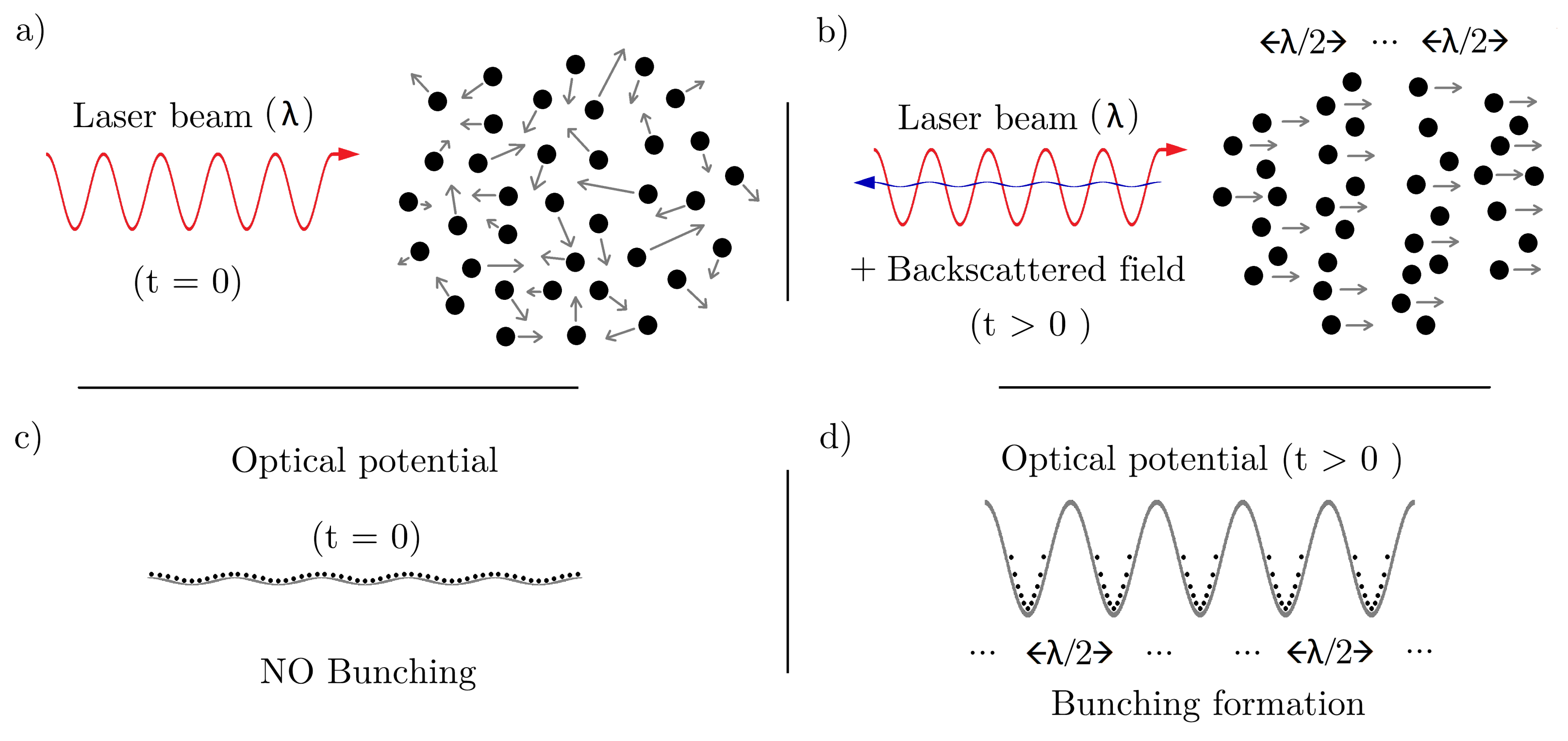
Initially, the atomic cloud, composed of many two-level atoms with negligible initial velocities and random positions, is illuminated by a far-detuned laser beam (see schematic in panel (a)).

–

Shortly after, a counter-propagating field arises from spontaneous scattering of pump photons (panel (b)). Now that there are two counter-propagating fields, they interfere to produce a small-amplitude standing wave that creates a periodic optical potential (panel (d)).

–

The potential starts to produce bunching (spatial modulation) in the cloud density by displacing the atoms, arranging them into bunches with a spatial period $\lambda /2$, where $\lambda$ is the wavelength of the pump field (panels (b) and (d)).

–

The bunching process and resultant atomic density grating is perceived by the pump as a polarization grating in the active medium, hence resulting in stimulated backscattering, i.e., into the probe field (the backscattered field is often termed ’probe’ even if it grows from noise).

–

Finally, the amplification of the probe triggers an amplification of the standing wave amplitude and hence the optical dipole potential depth. This causes further bunching that in turn results in additional backscattering.

The whole process is effectively a positive feedback loop, resulting in amplification of both the atomic density grating amplitude and the intensity of the backscattered probe field, which grows exponentially from initially tiny fluctuations.

Figure 1. CARL schematics illustrating: redistribution of atoms from (a) the initial random distribution to (b) spatially periodic density grating formation at time $t>0$. The density grating formation occurs simultaneously with the appearance of a spatially periodic optical dipole potential which is (c) initially shallow, but becomes deeper (d) as a consequence of the interference between the laser beam and the amplified backscattered light.

Figure 1. CARL schematics illustrating: redistribution of atoms from (a) the initial random distribution to (b) spatially periodic density grating formation at time $t>0$. The density grating formation occurs simultaneously with the appearance of a spatially periodic optical dipole potential which is (c) initially shallow, but becomes deeper (d) as a consequence of the interference between the laser beam and the amplified backscattered light.

The dipole force that stems from the interference between the pump and scattered fields produces two possibilities for the centre-of-mass motion of each atom during each scattering event. One possibility is that the atoms experience a double momentum kick in the forward direction (the pump propagation direction); one kick resulting from the scattering of a forward propagating pump photon, and another one due to the backscattering of a photon into the probe. The other possibility is that the atom may receive no momentum kick due to the forward scattering of a pump photon, which provides the atom with no recoil momentum. Under these circumstances, and using the photon picture of a scattering event, the two more likely atomic final momenta can be described by: $\hslash (k-[-k_0])\approx 2\hslash k$ and $\hslash (k-[+k_0])\approx 0$, respectively, where $k_0$ is the pump wavenumber, k is the probe wavenumber, and $k\approx k_0$. This scenario is depicted in Figure 1b, where the atomic cloud, initially containing stationary atoms, shows some bunching formation at a certain time t$>$0; there are some atoms moving forward with a momenta ∼$2\hslash k$ and others staying at rest with negligible momenta.

As it has been summarized, the CARL effect emerges when a cold atomic cloud is irradiated by a coherent optical field. Such a system has been shown to be characterized by two main responses: amplification of the probe due to backscattering from the atomic cloud, and self-organization of the atoms into a density grating with spatial period ∼$\lambda /2$. These two phenomena are closely coupled and are a consequence of the feedback of the system to an external stimulus. Early experimental evidence of backscattering due to formation of a wavelength-scale grating in an atomic cloud was demonstrated using a strongly pumped hot sodium vapor cell in [10,11], shortly after the idea of CARL was presented. In [10], the backscattering weakly amplified a seed field counterpropagating to the pump, whereas in [11], no seed field was present and strong amplification of backscattering initiated by noise was observed, simultaneous with the observation of a wavelength-scale grating in the atomic vapor. Aspects of both experimental studies could be understood in terms of different regimes of the CARL model developed by Bonifacio et al.; those of [10] by the low-amplification/gain limit where the atoms scatter independently with no collective enhancement and those of [11] by the high-gain limit where the atoms scatter collectively. The low-gain limit can also be interpreted in terms of recoil-induced resonance (RIR), proposed theoretically by Guo et al. [12,13] and observed experimentally by Courtois et al. in [14] using a cloud of cold Cs atoms illuminated by a pump laser and an almost co-propagating probe field. The theoretical idea of RIR presented by Guo describes absorption or emission of radiation taking atomic recoil into account, resulting in distinctive features in the probe gain spectrum termed RIR. A detailed theoretical comparison between RIR and CARL and the similarities and differences between them can be found in [15]. Although [10] and [11] demonstrated evidence consistent with backscattering from a wavelength-scale grating, Brown et al. [16] showed that many of these results could be explained using a model where the grating was one of atomic coherence rather than atomic density and which did not involve atomic recoil. Perrin et al. [17] showed that a coherence grating was more robust to the presence of atomic collisions than a density grating.

It was not until the early 2000’s that Kruse et al. presented the first unambiguous experimental evidence for CARL [18], by enclosing a collisionless cloud of ∼${10}^6$ ${}^{85}$Rb atoms at a temperature of several 100 $\mathsf{\mu }$K in a high-Q optical ring cavity. A significant difference between the setup used in these experiments from what was envisioned in the original CARL model was the use of optical molasses during the interaction, which introduced a friction force on the atoms and allowed this “viscous CARL” phenomenon to reach a steady-state [19].

After their observation of CARL [18] and RIR [20], Zimmermann’s group in Tubingen and colleagues showed that the (viscous) CARL experiments could be related to the Kuramoto model [21], the paradigm model for collective synchronization phenomena involving globally coupled oscillators [22]. In the case of CARL, the oscillators are moving atoms with a phase and frequency corresponding to atomic position and velocity, respectively, and the coupling is due to the evolving optical dipole potential which all the atoms experience. The threshold behavior observed in the CARL experiments were interpreted as a Kuramoto-like phase transition from an initial unsynchronized state to a final strongly synchronized state [21,23]. A detailed theoretical study of the relation between CARL and the Kuramoto model was presented in [24].

The original CARL model and its variants were semi-classical, describing the atomic gas as a collection of particle-like two-level atoms, whose centre-of-mass motion could be described classically. The extension of the CARL model to a fully quantum approach, by also describing the atomic center-of-mass motion quantum mechanically, was first carried out by Moore and Meystre [25]. This extension of the CARL model was needed because the semiclassical model breaks down when the temperature of the cloud is lower than the recoil temperature and the atoms are delocalised on the scale of the optical potential period, i.e., $\lambda /2$. In the late 1990s, the experimental realisation of Bose–Einstein Condensates (BECs) led to the observation of what was termed Superradiant Rayleigh Scattering (SRyS) when a BEC was illuminated by a far-detuned laser [9]. The extension of the CARL model showed theoretically that SRyS from a BEC can be described in terms of the CARL instability involving ultracold delocalised atoms [26]. The SRyS experiments stimulated several other closely related theoretical studies [27,28,29,30,31].

The quantum model was further developed by Bonifacio’s group and extended to the nonlinear regime [32] (later further extended in [33]), which showed good agreement with the experimental results obtained in [9]. In this work, a collective parameter, $\rho$, was introduced. This parameter depends on several quantities, e.g., detuning, pump intensity, relating to the atom-light coupling, but as will be shown later, its physical interpretation is the average number of scattered photons or, equivalently, the average number of momentum kicks each atom receives. The value of the collective parameter, $\rho$, allows a simple identification of whether the CARL process is essentially classical or quantum, i.e., whether it can be described using the original semiclassical CARL model or not. The system is in the quantum regime when the collective parameter, $\rho <1$, and it describes the situation where all atoms backscatter a single photon coherently. This model was used to study collective light scattering from BECs in different configurations: variation of the angle of incidence of optical field, extending the usual 1D model to a bidimensional 2D description [34]; studying quantum fluctuations and atom-photon entanglement [35]; propagation effects of short pulses [36]; accelerated CARL superradiance [37] and subradiance [38] using a two-frequency pump in an optical cavity.

This previous model was also used to compare superradiant Rayleigh scattering (SRyS) produced by a BEC in free space [9] with the recoil lasing effect observed using a BEC enclosed in a high-finesse cavity [39]. In this comparison, Slama et al. concluded that there is an intrinsic link between SRyS and CARL, which comes from tuning the cavity decay rate $\kappa$. CARL occurs when this cavity linewidth is smaller than the collective gain linewidth, $\kappa <{\omega }_r\rho$, resulting in scattered intensity $\propto {n_a}^{4/3}$, where $n_a$ is atomic density. When the cavity decay rate exceeds the collective gain linewidth, $\kappa >{\omega }_r\rho$, then the scattered field becomes superradiant in character with scattered intensity $\propto {n_a}^2$, i.e., SRyS occurs. A consequence of this is that as along as the atomic temperature is sufficiently low, there is no need for a cavity for SRyS to occur. The explanation is simple: when the cavity losses are above a threshold value, the coherence time is too short for the initial fluctuations to work as a seed for the probe, so they exit the cavity in form of superradiance. The experiment of [39] showed that CARL (and also SRyS) is not reliant on quantum statistics, but on cooperativity. This fact was further extended in a subsequent study by the same group [40].

During the last decade, the Tubingen group have carried out several other experiments related to CARL including investigation of the stability diagram of a BEC in an optical ring resonator and its connection with the Dicke phase transition [41], a similar investigation but involving thermal, cold atoms rather than BEC [42], observation of subradiant momentum states [43] and observation of supersolid properties [44].

2. CARL Model

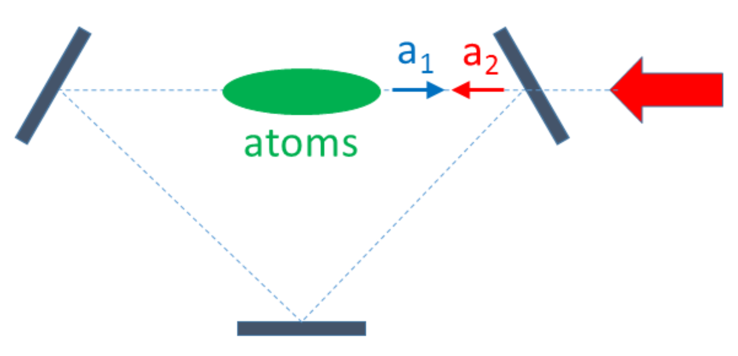
In CARL, the atoms interact with two counter-propagating electromagnetic fields (see Figure 2): (a) a pump beam with electric field $E_{2}cos(k_{2}z+{\omega }_{2}t)$, with frequency ${\omega }_2$ and a constant, intense Rabi frequency ${\Omega }_2=d_{eg}{E}_2/\hslash$, propagating along the negative direction of the cavity axis z; (b) a ’probe’ field with electric field $E_{1}cos(k_{1}z-{\omega }_{1}t+\varphi )$, with frequency ${\omega }_1$∼${\omega }_2$, slowly varying time-dependent Rabi frequency ${\Omega }_1\left(t\right)=d_{eg}{E}_1\left(t\right)/\hslash$ and phase $\varphi \left(t\right)$, propagating along the positive direction of the cavity axis z. The probe field is amplified by pump photons which are backscattered by the atoms, and eventually by an external seed signal. The interference between the two counter-propagating beams causes a dipole force on the atoms, in the limit $\Delta \gg \Gamma$ (where $\Delta ={\omega }_2-{\omega }_a$ is the pump-atom detuning) such that the scattering force is negligible. The dipole force, directed along the cavity axis z, is:

$$F=\frac{\hslash k}{\Delta }{\Omega }_1{\Omega }_{2}sin[2kz+({\omega }_2-{\omega }_1)t+\varphi ].$$

(1)

Notice that since ${\omega }_1$∼${\omega }_2$, we set $k_1+k_2$∼$2k$ and ${\omega }_2=\omega$ when appropriate.

Defining the position of the jth atom in terms of the phase ${\theta }_j=2k{z}_j$, and the momentum $p_j=m{v}_j$, where m is the atomic mass, $j=1,\cdots N$, and the ’pump-probe detuning’ $\delta ={\omega }_2-{\omega }_1$, the equations of motion for the atoms are:

$$\begin{array}{ccc}\hfill \frac{d{\theta }_j}{dt}& =& \frac{2k}{m}{p}_j,\hfill \end{array}$$

(2)

$$\begin{array}{ccc}\hfill \frac{d{p}_j}{dt}& =& \frac{\hslash k}{\Delta }{\Omega }_2{\Omega }_{1}sin({\theta }_j+\delta t+\varphi ).\hfill \end{array}$$

(3)

In these equations, the probe amplitude ${\Omega }_1$ and phase $\varphi$ evolve in time due to their interaction with the atoms. Introducing the complex Rabi frequency ${\tilde{\Omega }}_1={\Omega }_1{e}^{i\varphi }$, its dynamical equation in the mean-field approximation [5] is:

$$\frac{d{\tilde{\Omega }}_1}{dt}=i{\omega }_p^2\langle P_1+P_2{e}^{-i(\theta +\delta t)}\rangle -\kappa ({\tilde{\Omega }}_1-{\Omega }_{10}),$$

(4)

where ${\omega }_p=\sqrt{d_{eg}^2\omega n_a/2{ϵ}_0\hslash }$ is the effective ‘plasma’ frequency (with $n_a$ as the atomic density), $P_i=R_1^{\left(i\right)}+i{R}_2^{\left(i\right)}$ (with $i=1,2$) are the amplitudes of the polarization waves relative to the two fields, $\kappa$ is the cavity linewidth and ${\Omega }_{10}$ is an eventual injected signal. Notice the phase factor $e^{-i(\theta +\delta t)}$ multiplying $P_2$ in Equation (4) and containing the phase difference between the two counter-propagating beams, and the average $\langle \cdots \rangle =(1/N){\sum }_{j=1}^N(\cdots )$ over the N atoms. Assuming $\Delta \gg \Gamma$, such that $P_i\approx -{\Omega }_i/\Delta$, and ${\Omega }_2\gg {\Omega }_1$, Equation (4) becomes:

$$\frac{d{\tilde{\Omega }}_1}{dt}\approx -i\frac{{\Omega }_2}{\Delta }{\omega }_p^2{e}^{-i\delta t}\langle e^{-i\theta }\rangle -\kappa ({\tilde{\Omega }}_1-{\Omega }_{10}).$$

(5)

The probe field ${\tilde{\Omega }}_1$ in Equation (5) is driven by a collective term called bunching (or ‘optical magnetization’),

$$b=\langle e^{-i\theta }\rangle =\frac{1}{N}\sum _{j=1}^N{e}^{-i{\theta }_j}.$$

(6)

It can be considered as the order parameter of the system, describing the coherence in the emission process. At the beginning, the phases ${\theta }_j$ are distributed randomly and $b\approx 0$ (more precisely, the RMS value of b is $1/\sqrt{N}$). When the atoms are grouped within an optical wavelength, the atoms’ phases become correlated (as occurs in CARL) and $\left|b\right|$ becomes close to unity, strongly enhancing the emission process. Equations (2), (3) and (5) form the CARL equations, but they can be simplified into a dimensionless form. By introducing the dimensionless parameter $\rho$ (to be determined yet) and redefining the variables as follows: $\overline{t}=\left(8{\omega }_r\rho \right)t$, where ${\omega }_r=\hslash k^2/2m$ is the recoil frequency, and ${\overline{p}}_j=p_j/(2\hslash k\rho )=4k{v}_j/\left({\omega }_r\rho \right)$, the equations can be rewritten as

$$\begin{array}{ccc}\hfill \frac{d{\theta }_j}{d\overline{t}}& =& {\overline{p}}_j,\hfill \end{array}$$

(7)

$$\begin{array}{ccc}\hfill \frac{d{\overline{p}}_j}{d\overline{t}}& =& -i\frac{C_1}{{\rho }^2}\left\{{\tilde{\Omega }}_1{e}^{i\overline{\delta }\overline{t}}{e}^{i{\theta }_j}-\mathrm{c}.\mathrm{c}.\right\},\hfill \end{array}$$

(8)

$$\begin{array}{ccc}\hfill \frac{d{\tilde{\Omega }}_1}{d\overline{t}}& =& -i\frac{C_2}{\rho }{e}^{-i\overline{\delta }\overline{t}}\langle e^{-i\theta }\rangle -\overline{\kappa }{\tilde{\Omega }}_1;\hfill \end{array}$$

(9)

being $\overline{\delta }=\delta /\left(8{\omega }_r\rho \right)$, $\overline{\kappa }=\kappa /\left(8{\omega }_r\rho \right)$, $C_1={\Omega }_2/(32{\omega }_r\Delta )$, $C_2={\Omega }_2{\omega }_p^2/(8{\omega }_r\Delta )$ and where we have neglected the injected probe signal ${\Omega }_{10}$. Then, we determine the still-free parameter $\rho$ by defining the same dimensionless field $A=(i{C}_1{\tilde{\Omega }}_1/{\rho }^2)exp\left(i\overline{\delta }\overline{t}\right)$ in (8) and $A=(i\rho {\tilde{\Omega }}_1/C_2)exp\left(i\overline{\delta }\overline{t}\right)$ in (9). This transforms the CARL equations in a form with no free parameters other than $\overline{\kappa }$ and $\overline{\delta }$:

$$\begin{array}{ccc}\hfill \frac{d{\theta }_j}{d\overline{t}}& =& {\overline{p}}_j,\hfill \end{array}$$

(10)

$$\begin{array}{ccc}\hfill \frac{d{\overline{p}}_j}{d\overline{t}}& =& -\left(A{e}^{i\theta }+\mathrm{c}.\mathrm{c}.\right),\hfill \end{array}$$

(11)

$$\begin{array}{ccc}\hfill \frac{dA}{d\overline{t}}& =& \langle e^{-i\theta }\rangle +(i\overline{\delta }-\overline{\kappa })A.\hfill \end{array}$$

(12)

Equating the two definitions of A, we obtain $C_1{C}_2={\rho }^3$, so that

$$\rho ={\left(\frac{{\Omega }_2}{4\Delta }\right)}^{2/3}{\left(\frac{{\omega }_p}{4{\omega }_r}\right)}^{2/3}.$$

(13)

The scaled field amplitude is $\left|A\right|=|{\tilde{\Omega }}_1|/\sqrt{4\rho {\omega }_p^2}$. Using the definition of the plasma frequency ${\omega }_p=\sqrt{\omega d_{eg}^2{n}_a/2{ϵ}_0\hslash }$, where $n_a=N/V$ is the atomic density, and since $({ϵ}_0{E}_1^{2}V/2)/\hslash \omega$ is the average number of photons ${\langle N\rangle }_{\mathrm{photon}}$ in the volume V, then

$${\rho \left|A\right|}^2=\frac{{\langle N\rangle }_{\mathrm{photon}}}{N}$$

(14)

can be interpreted as the average number of photons scattered per atom.

Equations (10)–(12) have the same form of the equations for a free electron laser (FEL) [6], with differently defined dimensionless variables and parameters. In CARL, the incident photons of the pump are backscattered by the atoms, which recoil collectively. These equations, in the case of negligible cavity loss ($\overline{\kappa }\to 0$), admit a constant of motion expressing the conservation of the total momentum. From Equations (11) and (12), it follows that

$$\langle \overline{p}\rangle +{\left|A\right|}^2=\mathrm{constant},$$

(15)

i.e., the scattered field intensity grows when the average atomic momentum decreases. In dimensional variables, Equation (15) reads:

$$\sum _j{p}_j+(2\hslash k){\langle N\rangle }_{\mathrm{photon}}=\mathrm{constant}$$

(16)

The decrease in total atomic momentum equals the average number of scattered photons multiplied by the two-photon recoil momentum, $2\hslash k$.

3. CARL Instability

The CARL Equations (10)–(12) have an equilibrium state, corresponding to no scattered field, $A=0$, and no bunching, $b=0$. This equilibrium state is unstable for certain values of the detuning and cavity losses. This instability results in scattered field intensity and atomic bunching (i.e., a spatially periodic atomic density modulation) growing exponentially toward a different state. The onset of the instability can be obtained by a linear stability analysis of these equations.

By perturbing the equilibrium by small quantities, $A=\delta A$, ${\theta }_j={\theta }_{0j}+\delta {\theta }_j$ and ${\overline{p}}_j=\delta p_j$, with $\langle exp[-i{\theta }_{0j}]\rangle =0$, the linearized equations become:

$$\begin{array}{ccc}\hfill {\dot{\delta \theta }}_j& =& \delta p_j\hfill \end{array}$$

(17)

$$\begin{array}{ccc}\hfill {\dot{\delta p}}_j& =& -\left[\delta A{e}^{i{\theta }_{0j}}+\mathrm{c}.\mathrm{c}.\right]\hfill \end{array}$$

(18)

$$\begin{array}{ccc}\hfill \dot{\delta A}& =& -i\langle e^{-i{\theta }_{0j}}\delta {\theta }_j\rangle +(i\overline{\delta }-\overline{\kappa })\delta A.\hfill \end{array}$$

(19)

Defining the collective variables

$$\begin{array}{c}\hfill B=-i\langle e^{-i{\theta }_{0j}}\delta {\theta }_j\rangle \end{array}$$

(20)

$$\begin{array}{c}\hfill P=-i\langle e^{-i{\theta }_{0j}}\delta p_j\rangle \end{array}$$

(21)

the equations can be rewritten as:

$$\begin{array}{ccc}\hfill \dot{B}& =& P\hfill \end{array}$$

(22)

$$\begin{array}{ccc}\hfill \dot{P}& =& i\delta A\hfill \end{array}$$

(23)

$$\begin{array}{ccc}\hfill \dot{\delta A}& =& B+(i\overline{\delta }-\overline{\kappa })\delta A.\hfill \end{array}$$

(24)

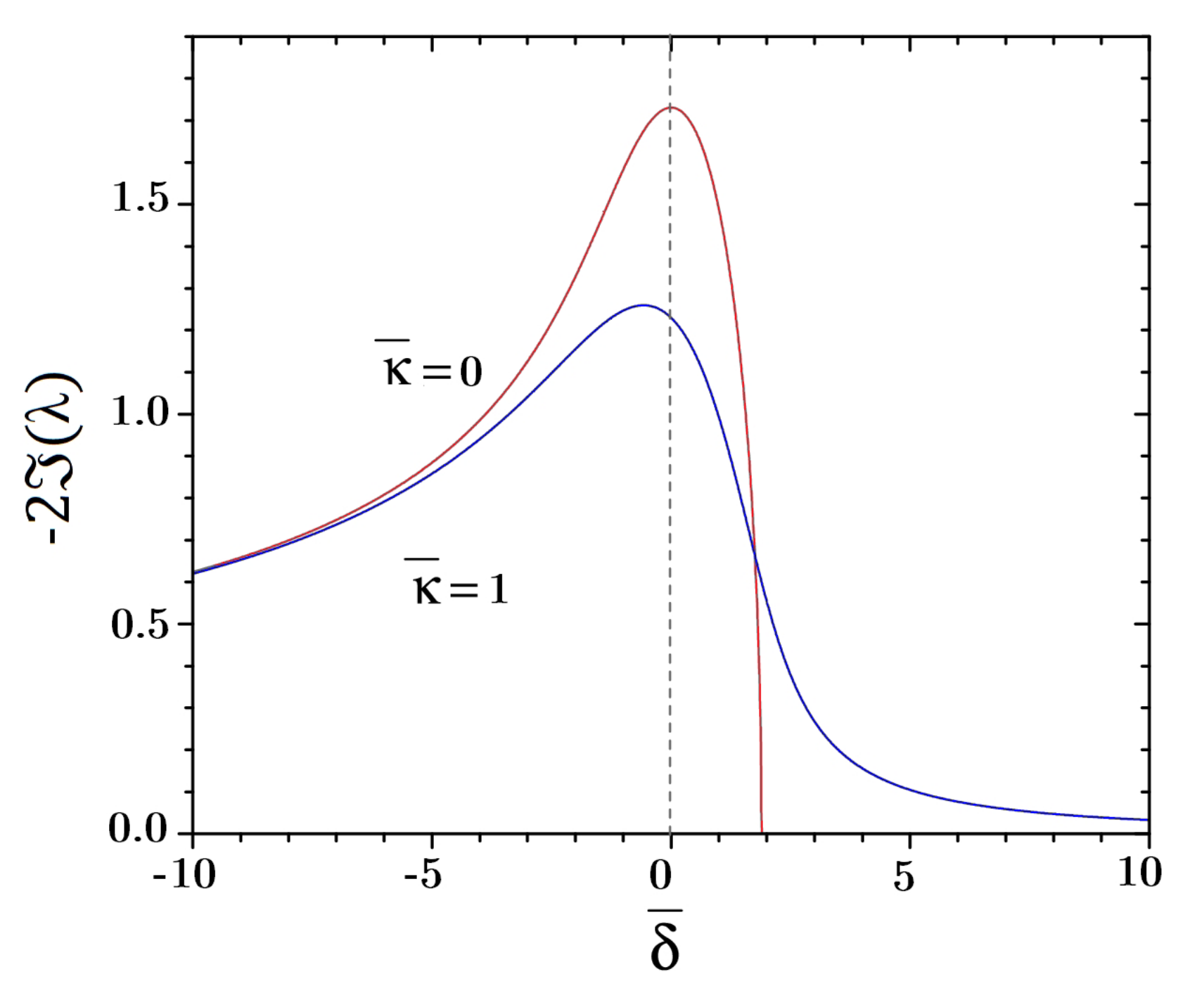
where we assumed that $\langle exp[-2i{\theta }_{0j}]\rangle =0$. The equations have been reduced to a system of three linear equations in the variables $\delta A$, B and P. Looking for solutions of the form $exp\left(i\lambda \overline{t}\right)$, where $\lambda$ is complex, we obtain the characteristic equation:

$${\lambda }^2(\lambda -\overline{\delta }-i\overline{\kappa })+1=0.$$

(25)

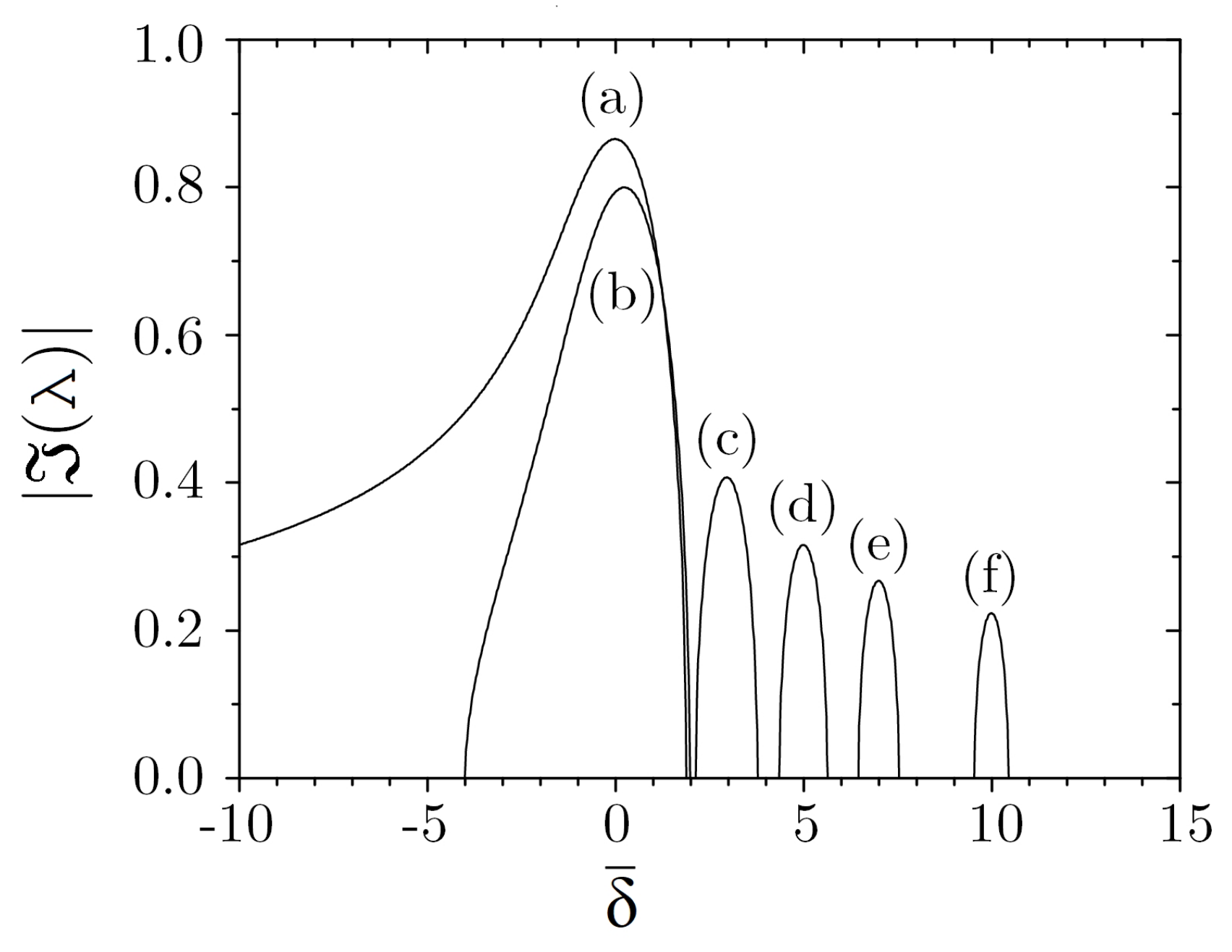
The system is unstable if $\lambda$ has a negative imaginary part. Figure 3 shows $-2\Im \left(\lambda \right)$ as a function of $\overline{\delta }$ for $\overline{\kappa }=0$ and $\overline{\kappa }=1$.

In the ‘good-cavity’ limit, $\overline{\kappa }\to 0$, the cubic equation has three real roots for $\overline{\delta }>{\delta }_T={(27/4)}^{1/3}$∼$1.89$, and one real and two complex conjugate roots for $\overline{\delta }<{\delta }_T$. The maximum growth (i.e., the maximum of $\Im \left(\lambda \right)$) occurs on resonance, $\delta =0$, with $\lambda =(1-i\sqrt{3})/2$. The intensity ${\left|A\right|}^2$ grows as $exp\left(\sqrt{3}\overline{t}\right)=exp\left(Gt\right)$, where $G=\sqrt{3}\left(8{\omega }_r\rho \right)$ is the exponential gain coefficient. $\Im \left(\lambda \right)$ is appreciably different from zero (where the field is amplified) only for $|\overline{\delta }|\le 2$, i.e., for $|{\omega }_2-{\omega }_1|\le 8{\omega }_r\rho$: this defines the CARL bandwidth $\Delta {\omega }_{\mathrm{CARL}}=8{\omega }_r\rho$, showing that only a limited range of frequencies around the pump frequency ${\omega }_2$ can be amplified. Since in the presence of an initial distribution of the atomic velocities the detuning is modified by the Doppler effect as $\delta =({\omega }_2+kv)-({\omega }_1-kv)={\omega }_2-{\omega }_1+2kv$, the probe field is amplified only if the CARL bandwidth is larger than the initial Doppler broadening, i.e., $k{\sigma }_v<4{\omega }_r\rho$. This sets a limit on the maximum temperature of the atomic gas such that CARL can occur. For instance, for ${\omega }_r$∼${10}^4{s}^{-1}$ and $\rho$∼${10}^2$, the maximum temperature the atomic gas (considering Rb atoms) can have is less than 10 $\mathsf{\mu }$K. For this reason, CARL was not clearly observed experimentally until denser, cold atomic clouds, such as those provided by a Magneto-Optical Trap (MOT), became available.

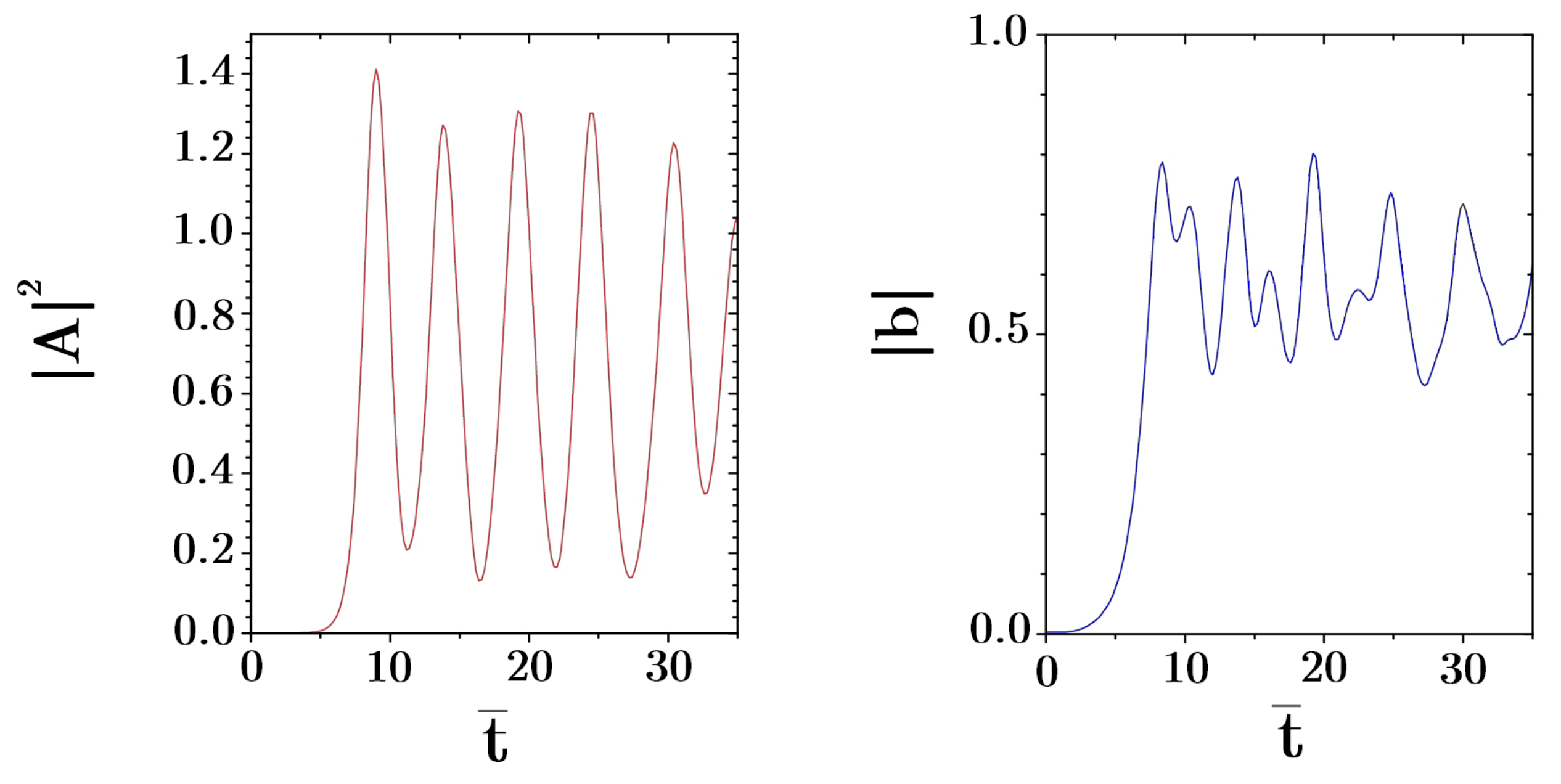
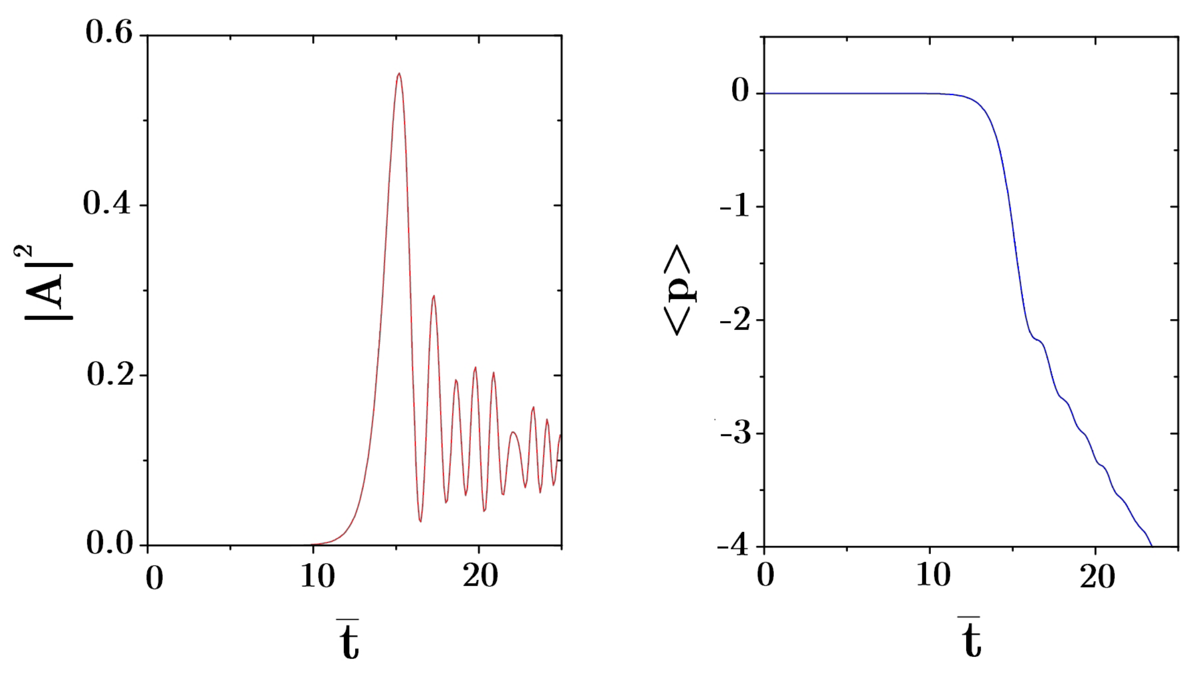
The complete dynamical evolution of scattered radiation and atoms can be obtained only by numerical integration of Equations (10)–(12). Figure 4 shows the scaled intensity ${\left|A\right|}^2$ and the bunching factor $\left|b\right|$ as a function of $\overline{t}$ for $\overline{\delta }=0$ and $\overline{\kappa }=0$.

The maximum scaled intensity is about $1.4$, meaning that each atom backscatters in average $1.4 \rho$ photons. The maximum bunching is about $0.8$ which corresponds to a well resolved density grating. Intensity and bunching show undamped nonlinear oscillations after the first maximum.

4. Superradiant CARL Regime

CARL may also operate in a superradiant regime [45,46], a phenomenon which shares some similarity with the better-known atomic superfluorescence [47] in two-level inverted atoms. It occurs in the ‘bad-cavity limit’, when the cavity losses are larger than the CARL bandwidth, i.e., $\kappa >\Delta {\omega }_{\mathrm{CARL}}$ or $\overline{\kappa }>1$. In this limit, the radiation amplitude adiabatically follows the slower atomic dynamics, so that, neglecting the time derivative in Equation (12),

$$\begin{array}{ccc}\hfill A& \approx & \frac{\langle e^{-i\theta }\rangle }{\overline{\kappa }-i\overline{\delta }},\hfill \end{array}$$

(26)

substituting for A in Equation (11) and averaging, we obtain

$$\frac{d\langle \overline{p}\rangle }{d\overline{t}}=-\frac{2\overline{\kappa }}{{\overline{\kappa }}^2+{\overline{\delta }}^2}{\left|b\right|}^2.$$

(27)

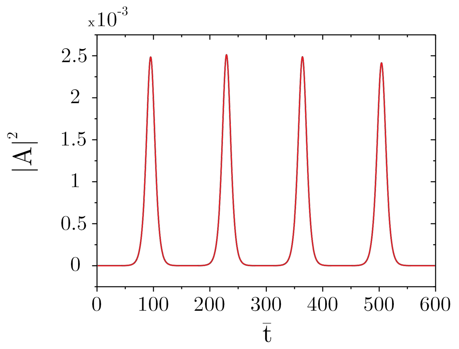
The average momentum continuously decreases in time. This means that the atoms backscatter photons into the cavity mode and these photons escape so quickly from the cavity that they can no longer be backscattered again into the pump mode. In this way, the average atomic momentum decreases monotonically. This behavior can be observed in Figure 5, which shows ${\left|A\right|}^2$ and $\langle \overline{p}\rangle$ as a function of time, for $\overline{\kappa }=1$ and $\overline{\delta }=0$. The maximum growth rate is close to $\overline{\delta }=0$ (see Figure 3).

For $\overline{\delta }=0$ the maximum scaled intensity is $|A_{\max }{|}^2\sim 1/{\overline{\kappa }}^2$ and, from Equation (14), the maximum number of scattered photon is

$${\langle N\rangle }_{\mathrm{photon}}\sim {\left(\frac{8{\omega }_r}{\kappa }\right)}^{2}N{\rho }^3={\left(\frac{{\Omega }_2}{2\Delta }\right)}^2{\left(\frac{{\omega }_p}{\kappa }\right)}^{2}N\propto N^2.$$

(28)

The peak intensity is proportional to the square of the atomic number, i.e., it is superradiant. The exponential gain coefficient in the superradiant regime can be obtained from Equation (25) assuming $\overline{\delta }=0$ and $\overline{\kappa }\gg \lambda$, so that ${\lambda }^2=-i/\overline{\kappa }$ and $\lambda =(-1-i)/\sqrt{2\overline{\kappa }}$. From it, $G_{SR}\approx 8{\omega }_r\rho {(2/\overline{\kappa })}^{1/2}=({\Omega }_2/\Delta ){(4{\omega }_r/\kappa )}^{1/2}{\omega }_p\propto \sqrt{N}$. We observe that the superradiant rate is smaller than the rate in the ‘good-cavity’ regime by a factor ${(2/3\overline{\kappa })}^{1/3}$. Moreover, the dependence on N changes from $N^{1/3}$ in the ‘good-cavity’ limit to $N^{1/2}$ in the superradiant regime.

The mean-field model just described for CARL superradiance in an optical cavity can be applied to describe, in an approximate way, the CARL superradiance in free space from an elongated atomic sample [46]. For an atomic cloud with an ellipsoidal shape of length L and cross-sectional area S, we can assume in Equation (12) that $\overline{\delta }=0$ and $\kappa$∼$1/\tau =c/L$, where $\tau =L/c$ is the escape time of the light from the atomic sample. Therefore, the maximum number of scattered photons is

$${\langle N\rangle }_{\mathrm{photon}}\sim {\left(\frac{{\Omega }_2}{4\Delta }\right)}^2\left(\frac{\sigma }{S}\right)\Gamma \tau N^2,$$

(29)

where we set $n_a=N/LS$, we introduced the spontaneous decay rate $\Gamma =d_{ge}^2{k}^3/(3\pi {ϵ}_0\hslash )$ and we instert the resonant cross section $\sigma =3{\lambda }^2/2\pi$. Finally, the superradiant gain rate is:

$$G_{SR}\approx \frac{{\Omega }_2}{\Delta }\sqrt{\frac{\sigma }{S}N{\omega }_r\Gamma }.$$

(30)

The superradiant CARL is an example of a dissipative system driven far from equilibrium by an external source and where a self-ordering process occurs. Many other similar phenomena have been studied in the past under the topic of ‘synergetics’, as originally described by the pioneer of this field, H. Haken [48].

5. Quantum Model of CARL

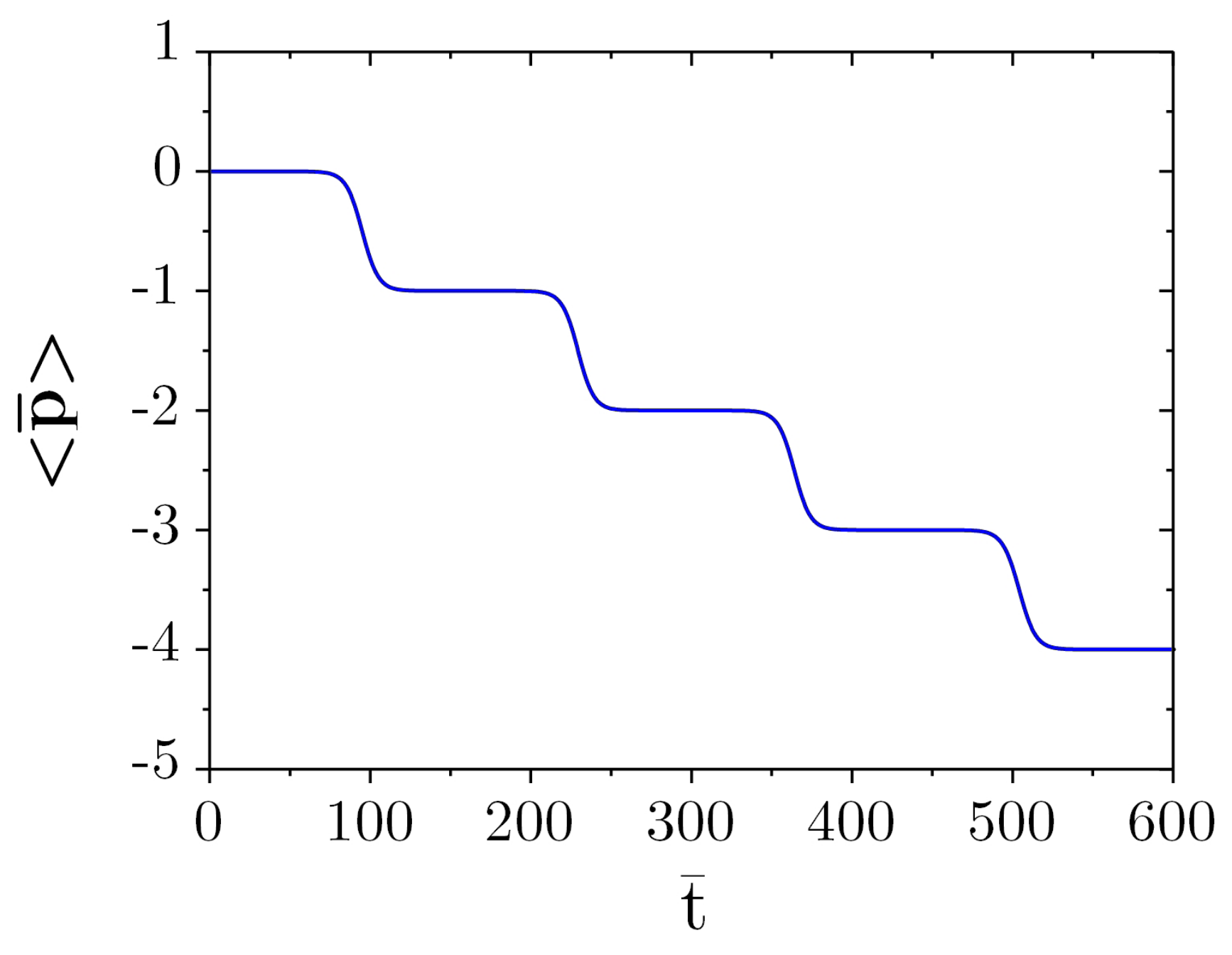
When the atoms are ultra-cold, below the recoil temperature $k_B{T}_{rec}={\hslash }^2{k}^2/2m$, they are unlocalized and behave as quantum-mechanical waves rather than classical point particles [49]. Then, the model derived in the previous section is no longer valid for describing the atomic centre-of-mass dynamics. When the atoms backscatter the monochromatic pump field, their momentum changes by an amount which is quantized in units of ($2\times$ the photon recoil momentum). Defining the atomic momentum in units of the two-photon recoil momentum $2\hslash k$,

$$p_{\theta j}=\frac{p_j}{2\hslash k}=\rho {\overline{p}}_j,$$

(31)

Equations (10)–(12) become

$$\begin{array}{ccc}\hfill \frac{d{\theta }_j}{d\overline{t}}& =& \frac{p_{\theta j}}{\rho },\hfill \end{array}$$

(32)

$$\begin{array}{ccc}\hfill \frac{d{p}_{\theta j}}{d\overline{t}}& =& -\rho \left(A{e}^{i\theta }+A^{*}{e}^{-i\theta }\right),\hfill \end{array}$$

(33)

$$\begin{array}{ccc}\hfill \frac{dA}{d\overline{t}}& =& \frac{1}{N}\sum _{j=1}^N{e}^{-i{\theta }_j}+(i\overline{\delta }-\overline{\kappa })A.\hfill \end{array}$$

(34)

Equations (32) and (33) can be derived from the Hamiltonian:

$$H=\sum _{j=1}^N\left[\frac{p_{\theta j}^2}{2\rho }-i\rho \left(A{e}^{i{\theta }_j}-A^{*}{e}^{-i{\theta }_j}\right)\right]=\sum _{j=1}^N{H}_j.$$

(35)

In order to describe the motion of the atoms quantum mechanically, we consider ${\theta }_j$ and $p_{\theta j}$ as canonical operators with $[{\theta }_j,p_{\theta j^{\prime }}]=(1/\hslash )[z_j,p_{z{j}^{\prime }}]=i{\delta }_{j{j}^{\prime }}$. We observe that the N atoms are independent, in an ‘external’ potential which depends on the self-consistent field A, assumed to be classical. Instead of solving the N Heisenberg equations for the operators ${\theta }_j\left(\overline{t}\right)$ and $p_{\theta j}\left(\overline{t}\right)$, we consider the Schrödinger equation for the wave function $\mathrm{\Psi }(\theta ,\overline{t})$, representing the statistical ensemble of the particles in a period of the potential, such that:

$${\int }_0^{2\pi }{\left|\mathrm{\Psi }(\theta ,\overline{t})\right|}^2=1.$$

(36)

Since $p_{\theta }\to -i\partial /\partial \theta$, the Schrödinger equation is [50]:

$$i\frac{\partial \mathrm{\Psi }(\theta ,\overline{t})}{\partial \overline{t}}=H_1\mathrm{\Psi }(\theta ,\overline{t})=-\frac{1}{2\rho }\frac{{\partial }^2\mathrm{\Psi }}{\partial {\theta }^2}-i\rho \left(A{e}^{i\theta }-A^{*}{e}^{-i\theta }\right)\mathrm{\Psi },$$

(37)

where $H_1$ is the single-particle Hamiltonian, and Equation (34) can be substituted by

$$\frac{dA}{d\overline{t}}={\int }_0^{2\pi }{\left|\mathrm{\Psi }(\theta ,\overline{t})\right|}^2{e}^{-i\theta }+i(\overline{\delta }-\overline{\kappa })A.$$

(38)

In Equation (38), the average $(1/N){\sum }_{j}exp(-i{\theta }_j)$ has been replaced by the ensemble average ${\int }_0^{2\pi }{\left|\mathrm{\Psi }(\theta ,\overline{t})\right|}^{2}exp(-i\theta )$, where $|\mathrm{\Psi }(\theta ,\overline{t}){|}^2$ can be interpreted as the atomic density of the periodic system of particles. Equations (37) and (38) form the simplest quantum model of CARL and its solution will be discussed in the next section. These equations describe the semiclassical behavior of a Bose–Einstein Condensate (BEC) in CARL.

Generally, a BEC is realized when N atoms become very close to each other, such that their wave functions overlap and the atoms become delocalized, forming a single, coherent, quantum macroscopic state. In a simplified picture, each atom is described by a wave packet of length equal to the De Broglie wavelength ${\lambda }_{DB}\sim h/p$, where $p=\sqrt{m{k}_{B}T}$ is the RMS momentum. The transition to the condensate phase occurs for low T (and hence low p) and high density. The condition is approximately that the number of atoms in a volume ${\lambda }_{DB}^3$ is larger than unity, $n_a{\lambda }_{DB}^3>1$, i.e., the temperature below a critical value depending on the density:

$$T<T_c=\frac{m{\hslash }^2{n}_a^{2/3}}{k_B}.$$

For $T<T_c$, the atoms start to occupy the lowest energy state with $p=0$ (hence $T=0$) until all the atoms have $p=0$ and the collective wavefunction extends across the entire condensate volume, which is determined by the trap potential and by the atom-atom collisions.

In the present case, we assume that the atomic gas is so dilute that the atom-atom interaction (corresponding to the cubic term in the Gross–Pitaevskii equation) can be neglected. Since for the Heisenberg uncertainty principle ${\sigma }_z{\sigma }_{p_z}$∼ℏ, in the condensate state ${\sigma }_{p_z}$∼$\hslash /L$, L is the size of the condensate. The quantum regime of CARL occurs when the momentum spread is smaller than the two-photon recoil momentum, $2\hslash k$, so when $\hslash /L\ll 2\hslash k$, i.e., when $L\gg \lambda$. For a condensate with a length much larger than the optical wavelength, the momentum spread due to the Heisenberg uncertainty principle can be neglected and the atoms can be assumed completely delocalized in a radiation wavelength, i.e., initially in the zero momentum state $|p_z=0\rangle$, with $\mathrm{\Psi }(\theta ,0)=1/\sqrt{2\pi }$.

Since $\theta$ is a periodic variable between 0 and $2\pi$ and $\mathrm{\Psi }$ is initially uniform, we can expand $\mathrm{\Psi }(\theta ,\overline{t})$ in a Fourier series:

$$\mathrm{\Psi }(\theta ,\overline{t})=\frac{1}{\sqrt{2\pi }}\sum _{m=-\infty }^{+\infty }{c}_m\left(\overline{t}\right)e^{im\theta }.$$

(39)

Quantum mechanically, $u_m=\langle \theta |m\rangle =\frac{1}{\sqrt{2\pi }}exp\left(im\theta \right)$ are the eigenfunctions of the momentum operator p with eigenvalues m. Therefore, the momentum values are multiples of $2\hslash k$ and $|c_m\left(\overline{t}\right){|}^2$ is the probability of finding the atoms with a momentum $m(2\hslash k)$. 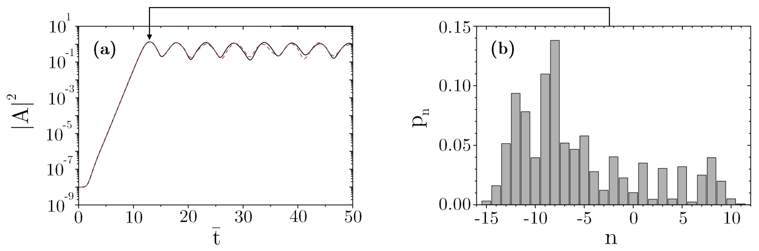Considering expression (39), Equations (37) and (38) become [32]:

$$\begin{array}{ccc}\hfill \frac{d{c}_m}{d\overline{t}}& =& -i{\displaystyle \frac{m^2}{2\rho }}{c}_m-\rho \left(A{c}_{m-1}-A^{*}{c}_{m+1}\right),\hfill \end{array}$$

(40)

$$\begin{array}{ccc}\hfill \frac{dA}{d\overline{t}}& =& \sum _{m=-\infty }^{\infty }{c}_m{c}_{m-1}^{*}+(i\overline{\delta }-\overline{\kappa })Al.\hfill \end{array}$$

(41)

The first equation describes transitions between the adjacent momentum states $|m\rangle$, induced by the interaction with the radiation field, whereas the second equation describes the evolution of the radiation field due to the bunching, seen now as a superposition of different momentum states.

6. Classical and Quantum Regimes of CARL

As was carried out for the classical equations, we now study the linear regime in order to investigate the stability of the equilibrium solution of Equations (40) and (41) with $A=0$ and $c_m\left(0\right)={\delta }_{m0}$; that is, atoms with initial zero momentum and completely delocalized in position, uniformly spatially distributed over $\lambda /2$ (i.e., $\mathrm{\Psi }(\theta ,0)=1/\sqrt{2\pi }$). By perturbing this equilibrium, we obtain three coupled equations for the first-order quantities $c_1$, $c_{-1}^{*}$ and A:

$$\begin{array}{ccc}\hfill \frac{d{c}_1}{d\overline{t}}& =& -i{\displaystyle \frac{1}{2\rho }}{c}_1-\rho A,\hfill \end{array}$$

(42)

$$\begin{array}{ccc}\hfill \frac{d{c}_{-1}^{*}}{d\overline{t}}& =& i{\displaystyle \frac{1}{2\rho }}{c}_{-1}^{*}+\rho A,\hfill \end{array}$$

(43)

$$\begin{array}{ccc}\hfill \frac{dA}{d\overline{t}}& =& c_1+c_{-1}^{*}+(i\overline{\delta }-\overline{\kappa })A.\hfill \end{array}$$

(44)

Looking for a solution of the form $exp\left(i\lambda \overline{t}\right)$, where $\lambda$ is complex, we obtain the characteristic equation:

$$(\lambda -\overline{\delta }-i\overline{\kappa })\left({\lambda }^2-\frac{1}{4{\rho }^2}\right)+1=0.$$

(45)

We note that the latter cubic expression reduces to the classical cubic, Equation (25), in the limit $\rho \to \infty$, i.e., when each atom scatters many photons on average. Figure 6 shows the imaginary part of $\lambda$, solution of Equation (45), as a function of $\overline{\delta }$ for $\overline{\kappa }=0$ and for different values of $\rho$: (a) corresponds to the classical solution, for $\rho \to \infty$; when $\rho <1$, $|\Im (\lambda \left)\right|$ has a maximum around $\overline{\delta }=1/2\rho$ and decreases as $\sqrt{\rho }$ (see curves (c)–(f)). The quantum regime of CARL occurs (in the ‘good-cavity limit’ $\overline{\kappa }\to 0$) when $\rho <1$; when every atom scatters (in the classical picture) less than a single photon. Since this is not possible in a quantum theory, the classical description breaks down and we enter in the quantum regime where every atom scatters exactly a single photon. It is at this low scattering rate that the discrete nature of the scattering process manifests, resulting from a succession of single photon scattering events.

6.1. Classical Regime

When $\rho \gg 1$, the average number of scattered photons per atom is large and the behavior becomes classical, with an almost continuous transfer of photons from the pump to the reverse cavity mode. The results of numerical integration of Equations (40) and (41) for $\overline{\kappa }=0$, $\rho =10$ and $\overline{\delta }=1/2\rho$, are shown in Figure 7. On the one hand, Figure 7a displays ${\left|A\right|}^2$ (on a log scale) vs. $\overline{t}$: the solution agrees with that obtained from the classical model (red line). On the other hand, Figure 7b illustrates the momentum distribution $p_n={\left|c_n\right|}^2$ at the maximum intensity; the momentum distribution is broad and shifted toward negative values, approximately with a width ${\sigma }_{\overline{p}}$∼$\rho$. It means that every atom has scattered a number of pump photons approximately equal to $\rho$, recoiling by approximately $-(2\hslash k)\rho$, but also increasing its momentum spread.

6.2. Quantum Regime

6.2.1. ‘Good-Cavity’ Quantum Regime

In the good-cavity limit $\overline{\kappa }\to 0$ we can write the cubic Equation (45) as

$$(\lambda -\overline{\delta })\left(\lambda -\frac{1}{2\rho }\right)\left(\lambda +\frac{1}{2\rho }\right)+1=0.$$

For $\rho \ll 1$, the equation can be solved assuming $\lambda =1/2\rho +x$, with $x\ll 1/\rho$. Hence, the equation becomes approximately

$$x^2-{\delta }^{\prime }x+\rho =0,$$

where ${\delta }^{\prime }=\overline{\delta }-1/2\rho$, with solutions $x_{\pm }={\delta }^{\prime }/2\pm (1/2)\sqrt{{\delta }^{\prime 2}-4\rho }$. If $|{\delta }^{\prime }|<2\sqrt{\rho }$ the two solutions are complex conjugates,

$${\lambda }_{\pm }=\frac{1}{2\rho }+\frac{{\delta }^{\prime }}{2}\pm \frac{i}{2}\sqrt{4\rho -{\delta }^{\prime 2}},$$

with maximum imaginary part equals to $\sqrt{\rho }$ at ${\delta }^{\prime }=0$, i.e., $\overline{\delta }=1/2\rho$. This resonance condition corresponds to the relation

$${\omega }_1={\omega }_2-4{\omega }_r,$$

(46)

which expresses conservation of energy: when a pump photon is absorbed and a probe photon is emitted, the atom recoils with momentum $2\hslash k$ and energy $E_r={(2\hslash k)}^2/2m=4\hslash {\omega }_r$. The recoil-frequency shift is a purely quantum effect and it is not present in the classical picture. The two resonances $\lambda =\pm 1/2\rho$ can be interpreted as energy shifts of $\pm 4{\omega }_r$, respectively, related to the energy shift due to the backscattering of a pump photon and to its reverse process. The only unstable process in the quantum regime of CARL is the former. It is important to note that in order to observe this regime, the Doppler shift due to the initial momentum spread of the atoms must be smaller that the recoil shift $4{\omega }_r$. Therefore, it is necessary to have a sub-recoil temperature in order to observe the quantum regime of CARL. Furthermore, since every atom coherently scatters a single photon, no further momentum spread is induced in the process, contrary to what happens in the classical regime, where many photons are scattered by each atom.

Due to the resonance condition, the atoms emit photons populating the momentum state $m=-1$, without the possibility of populating the opposite momentum state $m=1$, associated with the absorption of a probe photon and emission of a photon into the pump mode. This asymmetry implies that the condensate behaves as a two-level system, with a transition from the momentum states $m=0$ to the momentum state $m=-1$, in a similar way as happens in a laser, where the initial state $m=0$ corresponds to the excited state of the two-level atom. The main difference here is that for the momentum states there is not in general a decay mechanism for which the atom spontaneously leaves the state $m=0$ to decay into the state $m=-1$, so consequently the interaction remains coherent. Formally, the multi-level Equations (40) and (41) in the quantum regime of CARL become those for a transition from the level m to the level $m-1$ with $m=0,-1,\cdots$:

$$\begin{array}{ccc}\hfill \frac{d{c}_m}{d\overline{t}}& =& -i{\displaystyle \frac{m^2}{2\rho }}{c}_m-\rho A{c}_{m-1},\hfill \end{array}$$

(47)

$$\begin{array}{ccc}\hfill \frac{d{c}_{m-1}}{d\overline{t}}& =& -i{\displaystyle \frac{{(m-1)}^2}{2\rho }}{c}_{m-1}+\rho A^{*}{c}_m,\hfill \end{array}$$

(48)

$$\begin{array}{ccc}\hfill \frac{dA}{d\overline{t}}& =& c_m{c}_{m-1}^{*}+(i\overline{\delta }-\overline{\kappa })A.\hfill \end{array}$$

(49)

The resonance condition for this transition is obtained for $\overline{\delta }=(1-2m)/2\rho$, i.e., when ${\omega }_2-{\omega }_1=4{\omega }_r(1-2m)$ with $m=0,-1,\cdots$. In Figure 8, we show the scaled intensity ${\left|A\right|}^2$ as a function of $\overline{t}$, as obtained from the numerical integration of Equations (40) and (41) for $\overline{\kappa }=0$, $\rho =0.1$ and $\overline{\delta }=1/2\rho$. The peak intensity value is $|A_{\mathrm{peak}}{|}^2=1/\rho$, i.e., the number of scattered photons is ${\langle N\rangle }_{\mathrm{photon}}=N$: every atom scatters exactly one photon at the peak. It is possible to demonstrate that the radiation field is a $2\pi$ pulse, with the typical hyperbolic secant profile [32].

6.2.2. Superradiant Quantum Regime

Similarly to the classical regime, the quantum regime also offers the possibility of superradiant behavior. The features of the regime are very close to these of atomic superfluorescence [51]. Returning to the cubic Equation (45), assuming $\overline{\kappa }\gg \overline{\delta },\lambda$, and $\lambda =1/2\rho +x$ with $x\ll 1/\rho$, we obtain

$$\lambda \sim \frac{1}{2\rho }-i\frac{\rho }{\overline{\kappa }}$$

(50)

The growth rate in the quantum superradiant regime is

$$G_{SR}=(-2\Im \left(\lambda \right))\left(8{\omega }_r\rho \right)={\left(\frac{{\Omega }_2}{\Delta }\right)}^2\left(\frac{{\omega }_p^2}{2\kappa }\right).$$

(51)

The superradiant quantum regime occurs when the growth rate is less than the recoil shift, i.e., $G_{SR}<8{\omega }_r$ or equivalently when $\rho <\sqrt{\overline{\kappa }}$ (which is a less stringent than the ‘good-cavity’ condition $\rho <1$) [52]. In order to illustrate the quantum superradiant regime of CARL, Figure 9 shows the numerical solution of average scaled momentum $\langle \overline{p}\rangle ={\sum }_{m}m{\left|c_m\right|}^2$ vs. $\overline{t}$ for $\overline{\kappa }=10$, $\rho =1$ and $\overline{\delta }=0.5$. The average momentum changes toward negative values by steps of $2\hslash k$, corresponding to sequential superradiant transitions from the momentum state m to $m-1$ with $m=0,-1,\cdots$.

6.2.3. Entanglement

In this review, we have concentrated mainly on models of CARL in which the optical field is described classically, so that even the ‘quantum’ regime described in this section is strictly speaking semiclassical, as only the atomic dynamics is treated quantum mechanically. However, several studies of the quantum regime of CARL also included a quantum description of the optical field, resulting in a fully quantum treatment which allowed the study of correlations during the interaction. It has been demonstrated in [35,53] that the strong correlations between single-mode photons and atoms in defined momentum states allow the creation of photon–atom and atom–atom entangled states. In these works, it was shown that three-mode entanglement as well as two-mode atom–atom and atom–radiation entanglement are generally robust against losses and decoherence, thus making the quantum CARL system a good candidate for the experimental observation of entanglement in BEC systems. In particular, steady-state entanglement may be obtained both between atoms with opposite momenta and between atoms and photons.

7. Experimental Evidence for CARL

CARL has been demonstrated in both the thermal [18] and the ultracold regime [40] in a series of experiments carried on in Tübingen, in the group of C. Zimmermann, at the same time providing the first experimental realization of a BEC inside a ring optical cavity.

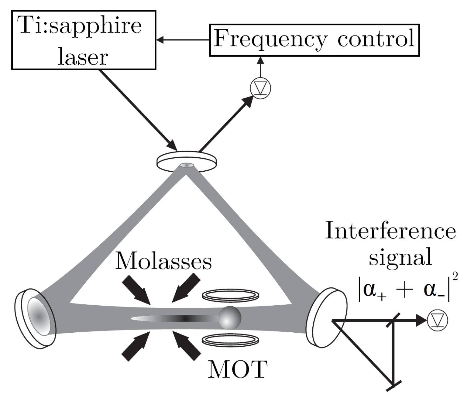
More specifically, a ring cavity supports a pair of degenerate, counterpropagating running-wave modes. The atomic gas is trapped at the position of the cavity modes, where one of them is pumped through one of the cavity mirrors (see Figure 10). Photons injected into the forward-propagating cavity mode are scattered back via the atoms into the unpumped, counterpropagating cavity mode, while the atoms recoil. Exponential gain of this unpumped, counterpropagating field then triggers the CARL instability.

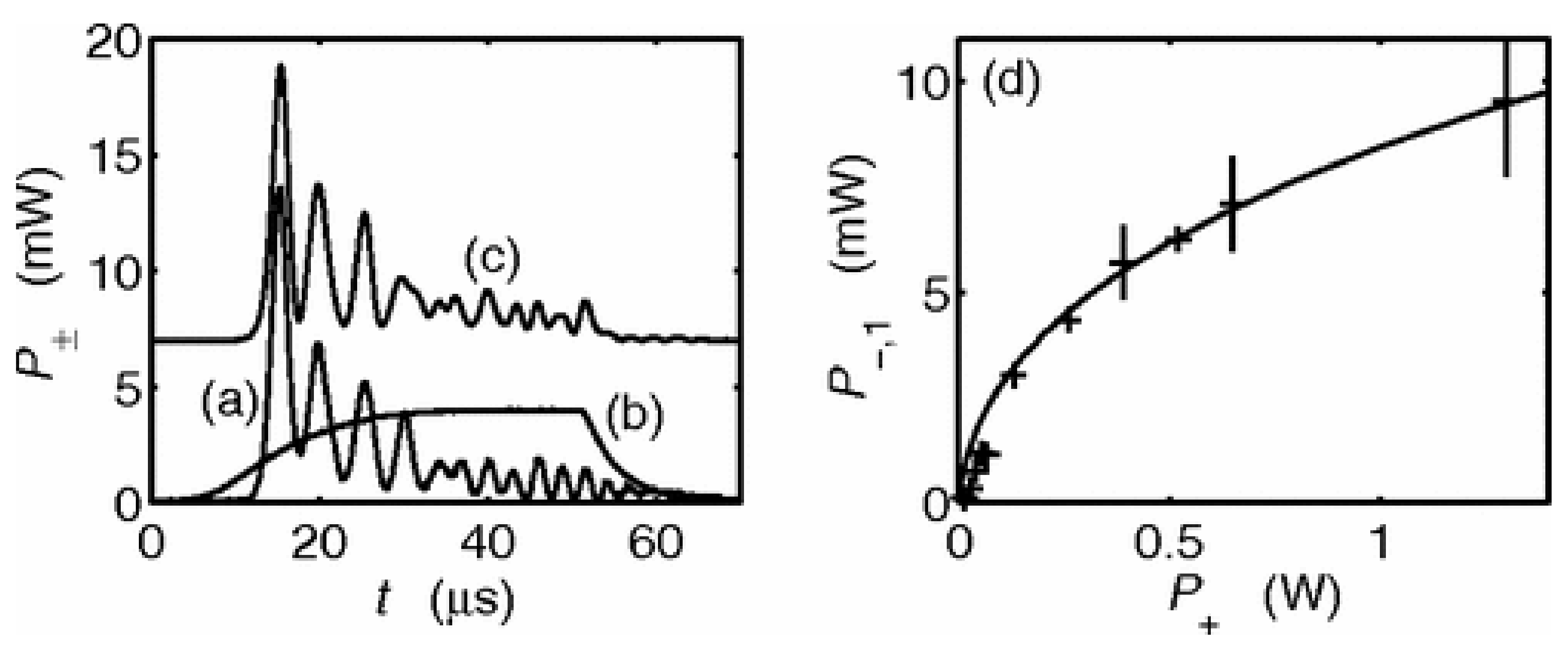
With the described setup, the Tübingen group observed CARL in both the bad-cavity and good-cavity regime [32]. The observed characteristics of the instability allowed for clear identification of the two regimes and showed the intrinsic connection between CARL and superradiant Rayleigh (SRyS) scattering [54]. In a former experiment with $T=100$ mK cold atoms [39] and in a successive experiment [40], where the temperature was varied between values of $T=1$ mK and $T=40\mathsf{\mu }$K [55,56] (see Figure 11 and Figure 12), the Tübingen group proved experimentally that CARL and hence also SRyS do not require quantum degeneracy of the atoms, but rely only on the cooperative behavior of the atoms [57].

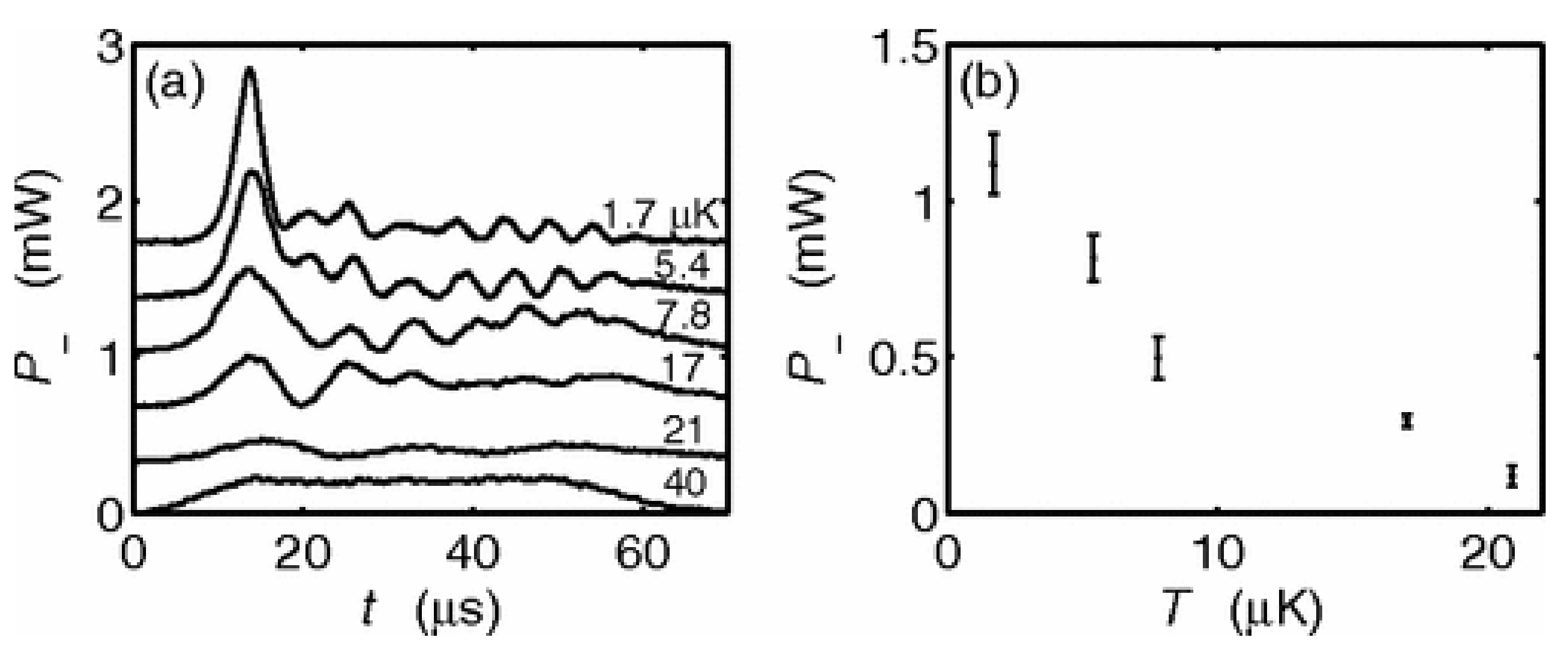
More specifically, the experiments [39,40] were able to examine the transition between the regimes described in the previous sections by changing the finesse of the cavity. As already discussed, what discerns the good-cavity from the bad-cavity regime is the size of the cavity linewidth compared with the recoil frequency ${\omega }_r$. The linewidth determines the density of states inside the cavity and limits the range of frequencies accessible for the probe light field. The frequency of the scattered photons is, on the other hand, Doppler shifted with respect to the pump light frequency, which is locked to a cavity resonance. The size of the shift is given by the momentum of the scattering atoms. For that reason, a cavity linewidth which is smaller than the recoil frequency limits the atomic dynamics to the momentum state $|p_z=0\rangle$ and its closest neighbors (good-cavity regime). Conversely, if linewidth is larger than the recoil frequency, all momentum states which are lying within the linewidth may participate in the CARL dynamics. However, how the dynamics take place is determined by the gain bandwidth (equal to $\Delta {\omega }_{CARL}=8{\omega }_r\rho$ in the good-cavity regime, $\overline{\kappa }\ll 1$ or to $G_{SR}$ in the bad-cavity regime, $\overline{\kappa }>1$. The ratio between the gain bandwidth and the recoil frequency determines how many momentum states are amplified at the same time. For example, if the ratio is smaller than one, which is called quantum regime, only two neighboring momentum states are coupled with each other. This leads to a coherent behavior, as in a two-level system, such that at any time, the momentum population is distributed to a maximum value of just two momentum states. However, if the ratio between the gain bandwidth and the recoil frequency is larger than one, which is called the semiclassical regime, several momentum states are coupled at a time. In this case, the initial momentum distribution, even if only one momentum state was occupied, as in a BEC, is spread over several momentum states by the dynamics. The occupation of more and more momentum states then leads to a decreasing bunching of the atoms and consequently to decoherence of the system.

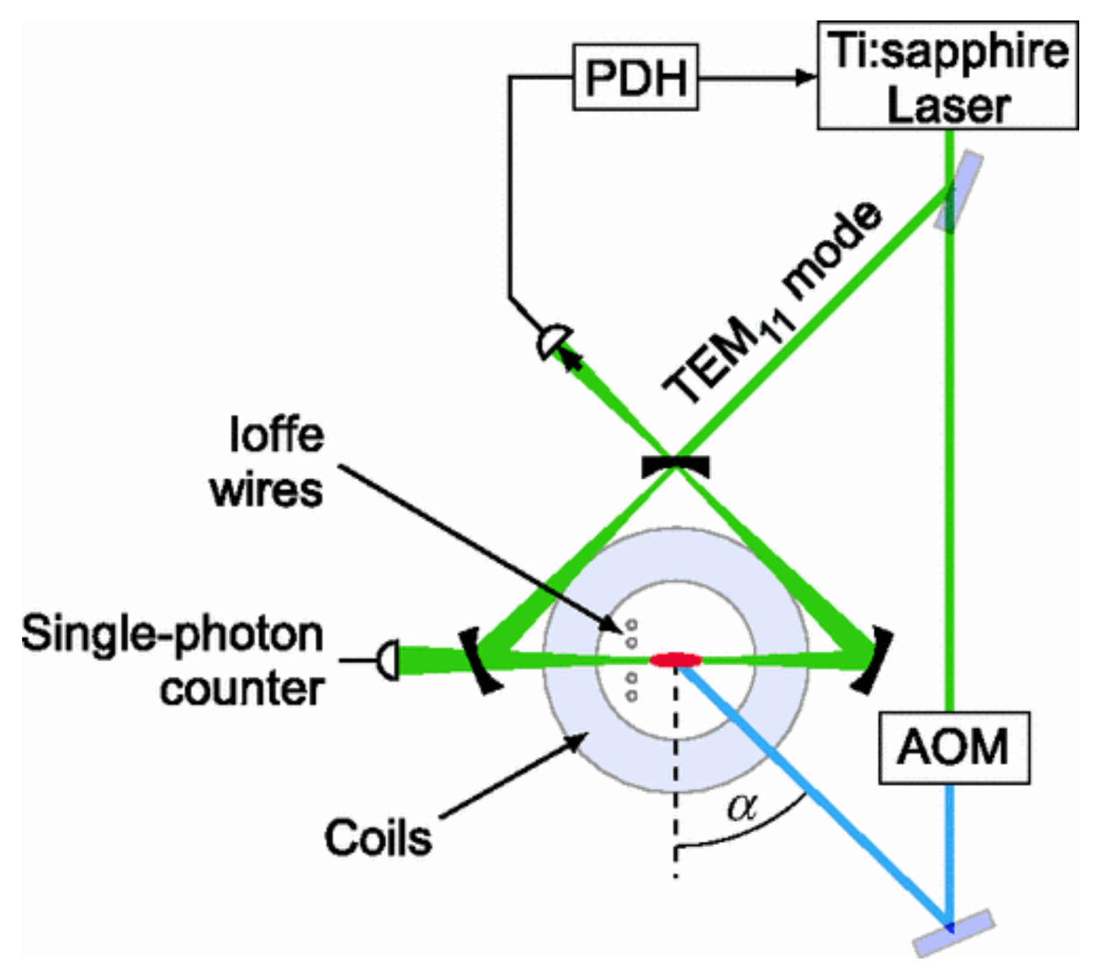
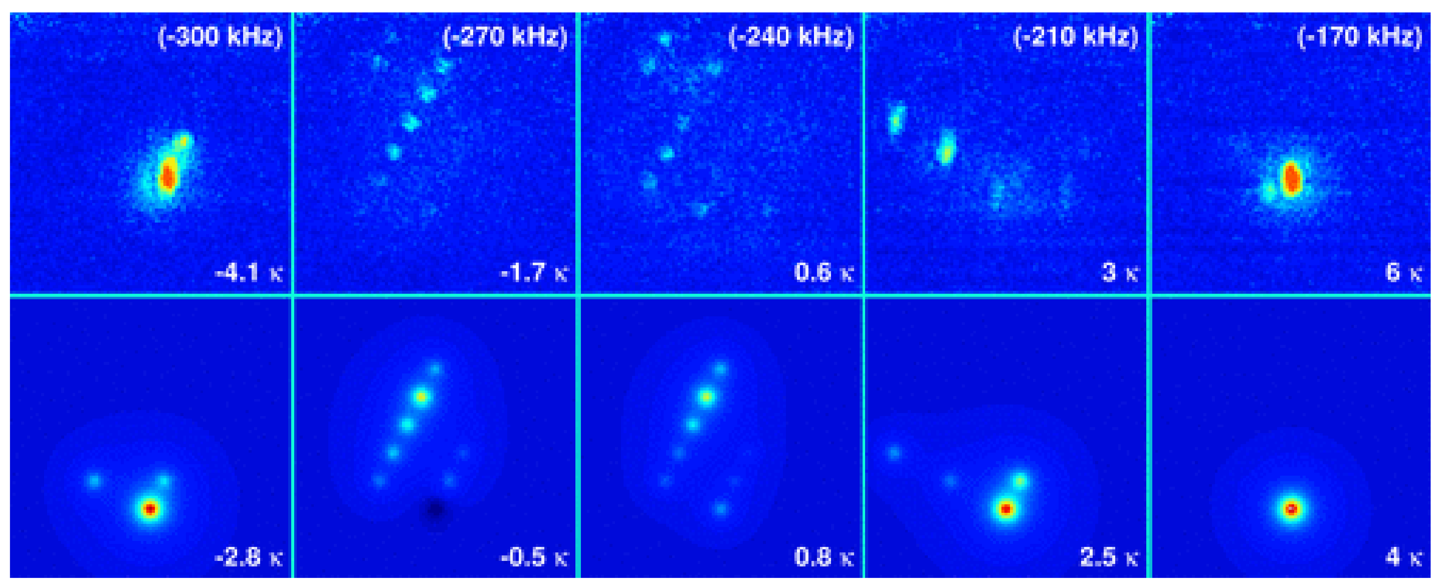
Further experiments investigated a new setup where a transversely pumped BEC cloud coupled to an initially empty ring resonator. Scattering from the transverse pump beam under an angle into the ring cavity leads to population of higher momentum modes. The main advantage of this configuration is that the pump frequency is no longer locked to a cavity resonance, so that the pump-cavity detuning can be experimentally controlled. The sideband-resolved regime, in which this resonator operates, allowed control of the population of specific momentum states by varying the detuning between the cavity resonance and the pump frequency [56,58] (see Figure 13 and Figure 14).

8. Conclusions

We conclude this review by mentioning some ways in which research on topics related to CARL have developed. CARL represents an early example of a phenomenon which involves the mechanical effects of light during its interaction with atoms and the backaction of the resulting atomic centre-of-mass motion on the optical field. It is, therefore, an early example of what would now be termed an optomechanical effect. Optomechanics is now a large and highly active field of research which encompasses the interaction between light and matter (ranging from microscopic atoms to macroscopic membranes or moving mirrors), involving the mechanical effect of light on matter and the consequent backaction of the moving matter on the optical field. Optomechanical interactions have been used as the basis for new nonlinear optical phenomena (e.g., spontaneous self-structuring of cold gases and BEC [59]) and potential applications as ultrasensitive detectors of inertial forces or displacements [60,61].

When CARL was first proposed in the mid-1990s, storing cold atoms in optical cavities was a significant challenge. Technical advances since then have realised many experiments worldwide which involve cold atoms and ultracold, quantum degenerate gases trapped in optical cavities, which have stimulated studies involving new methods for cooling atoms and other microscopic objects, self-organization processes, nonlinear dynamics, and quantum simulation. Details can be found in comprehensive reviews by Ritsch et al. [62,63]. However, as was demonstrated by the SRyS experiments, sufficient backaction for CARL and similar instabilities can occur in free space. Without a preferred scattering direction provided by a cavity axis, CARL interactions in free space generally involve scattering into multiple spatial modes rather than the single direction supported by a cavity. These multimode CARL interactions are the subject of current study for thermal clouds [64,65] and form part of recent advances in understanding of how large clouds of cold atoms interact collectively or cooperatively with light [66,67,68,69,70,71,72].