3.1. Ca II
Calcium (Ca) has 26 known isotopes, of which 5 are stable [
27].
43Ca has an abundance of only 0.135% but is the only stable isotope that has a hyperfine structure due to its non-zero nuclear spin
. The levels of interest in
43Ca II are the even [Ar]
and [Ar]
as well as the odd [Ar]
.
Due to its relatively simple electronic structure,
43Ca II has already been studied in depth theoretically by Silverans et al. [
28] and Yu et al. [
29] using the Relativistic Many-Body Perturbation Theory (RMBPT) approach, Itano [
8] with the MCDHF method, Chakraborty et al. [
30] with the Relativistic Coupled Cluster (RCC) method, and Safronova et al. [
31] using the relavistic all-order method, where all single, double, and partial-triple (SDpT) excitations of the wavefunctions are included to all orders of perturbation theory. Goble et al. [
9] and Nortershauser et al. [
1] performed optical spectroscopy experiments using hollow cathode discharge and fast ion beam collinear laser spectroscopy, whereas Garcia Ruiz et al. [
32] adopted bunched-beam collinear laser spectroscopy.
The MCDHF method used in this paper relies on the AS [
19] and LBL [
24] approaches, which enable the optimization of only a subset of orbitals in each calculation step. For example, for the ground
level, an initial Dirac–Hartree–Fock (DHF) layer is considered. This layer is built using the
spectroscopic orbitals in nonrelativistic notation, where the highest
n quantum number is quoted for each
l-symmetry, and no electron correlation is included at this stage. The ASs are then expanded with correlation orbitals up to
(
g-orbitals) to directly apply the Ba/Sr model [
15] and achieve high precision in the calculations [
33]. For each AS given in
Table 1, only the newly introduced orbitals are optimized, while the remaining orbitals are kept frozen. The mixing coefficients of the ASFs are then determined, and Quantum Electrodynamics (QED) corrections are included during the RCI step. Finally, the HFS constants are computed.
Following Bieroń et al.’s approach [
34], we investigated the impact of different classes of orbital substitutions. Via an DHF orbital basis, more correlations were accumulated by allowing single and double (SD) substitutions from deeper orbitals employing Single References (SRs) for each level using the fourth correlation layer (AS4) given in
Table 1.
In
Table 2, the individual contribution of single (S) orbital substitution to the magnetic dipole HFS constant of the ground level,
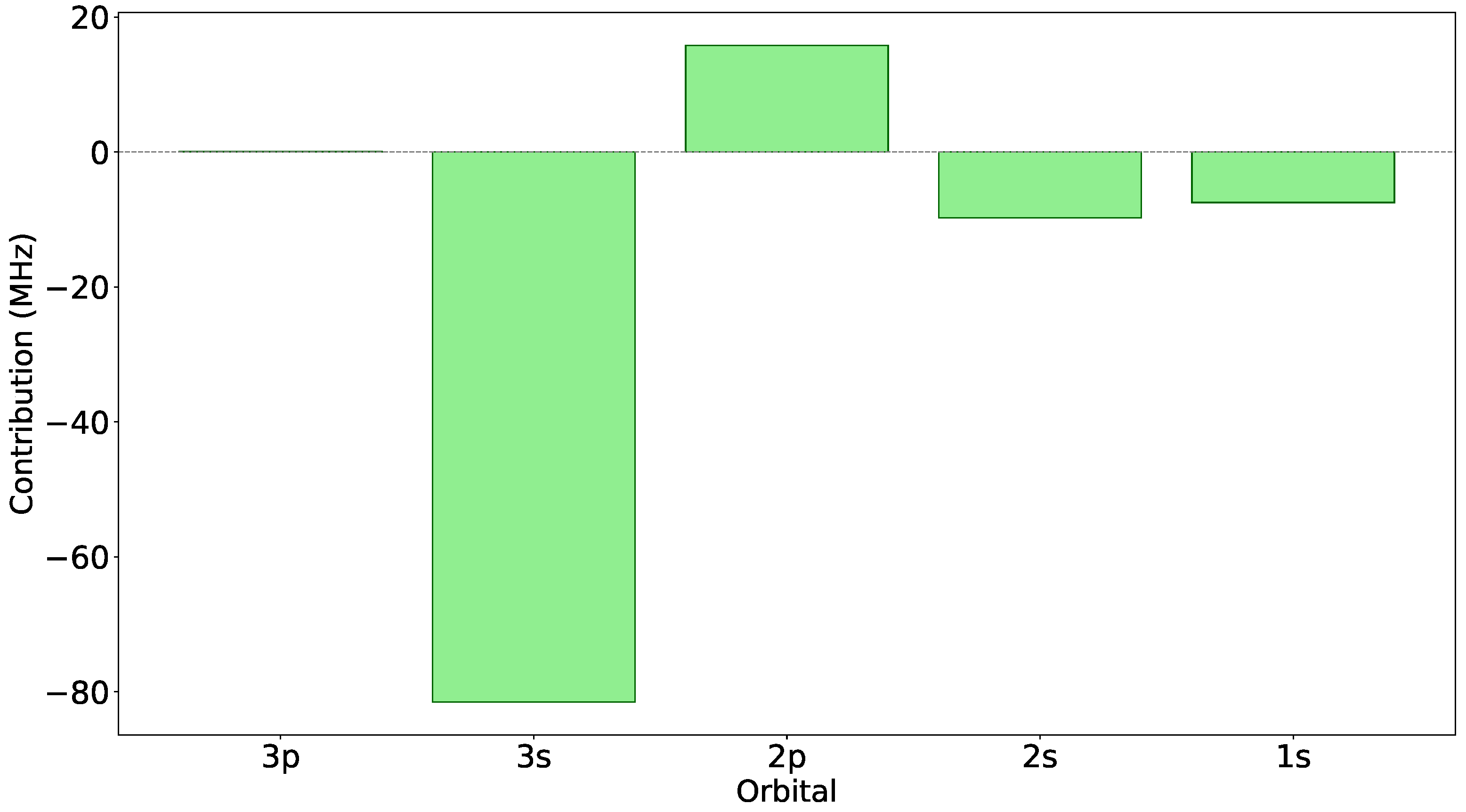
, is presented.
Figure 1 gives a more visual representation of these contributions.
While the contribution of the
orbital is negligible, namely, +0.08 MHz, the
s orbital substitutions dominate, with the
orbital contributing
MHz. This highlights the critical role of
s single substitutions in the HFS. To align with the Ba/Sr methodology [
15], the
and
orbitals are included in the optimization step, even though the
substitution contributes less than one percent. Consequently,
correlations are excluded from the optimization.
Table 2.
Contributions of occupied orbitals to the calculated values of A hyperfine constant for the level of 43Ca II. shows the individual contributions coming from the single (S) orbital substitutions.
Table 2.
Contributions of occupied orbitals to the calculated values of A hyperfine constant for the level of 43Ca II. shows the individual contributions coming from the single (S) orbital substitutions.
| Orbital | | A (MHz) | |
|---|
| | 1 | | |
| 32 | | |
| 2377 | | |
| 4303 | | |
| 12,455 | | |
| 16,468 | | |
Figure 1.
Contributions of single (S) orbital substitutions relative to the DHF constant in 43Ca II.
Figure 1.
Contributions of single (S) orbital substitutions relative to the DHF constant in 43Ca II.
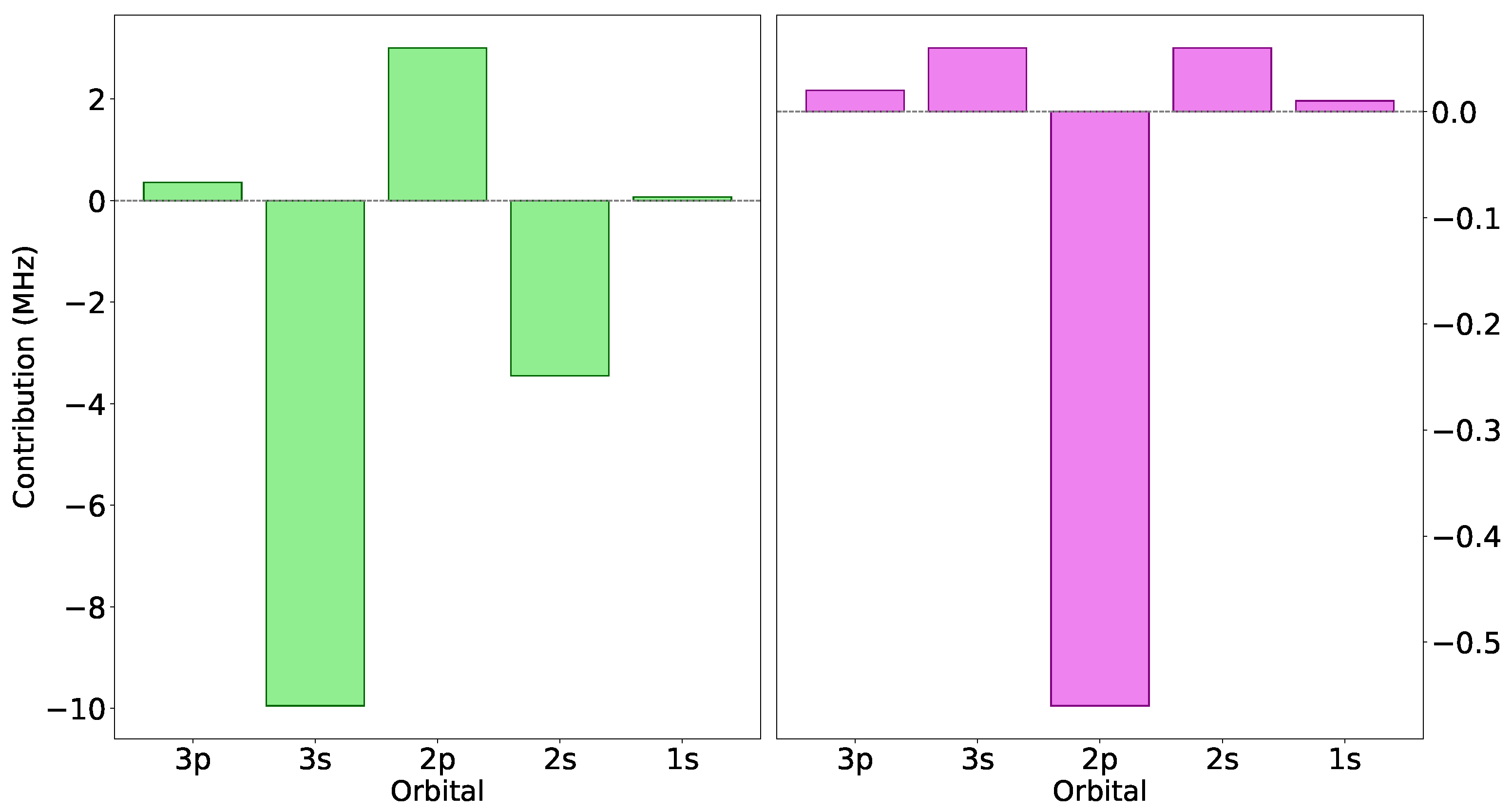
As shown in
Table 3 and
Figure 2, the contributions for the excited states are similar, with the
contribution being negligible compared to those of
and
. The contributions for the
B hyperfine constants indicate that the most important contribution comes from
correlations, which is mainly due to the orbital polarization or Sternheimer effect [
23]. The trends above are also observed in the
and the odd
P levels.
Thanks to this analysis, the optimization of the radial orbitals can be targeted for relevant correlations for the hyperfine structure. The GRASP package [
16] considers spectroscopic orbitals in two ways. Let us take the example of the ground
(or [Ar]
) level. The core orbitals are
, while the valence orbital is
. We can therefore build our MCDHF optimizations on core–valence (CV) correlations. To directly apply the MCDHF + RCI model developed for
87Sr II and
137Ba II [
15], we used the equivalent CV single and restricted double (SrD) orbital optimization strategy with
substitutions. Here, “restricted” means at most one hole per active core orbital, i.e., allowing substitutions from
and
to
, with a maximum of one substitution from each core orbital to the valence one [
35]. A second optimization strategy (MCDHF CV SrD
) addressing the
and
core orbitals important for correctly describing the HFS for the excited levels was also considered. With the ASs described in
Table 1, seven layers of correlation orbitals were considered in order to achieve convergence in our results. The latter is obtained when the HFS constants do not vary within some a priori-accepted variation interval. The results for the HFS constants in each optimization step are given in
Table 4.
Figure 2.
Contributions of single (S) orbital substitutions relative to the DHF (left, in light green) and (right, in violet) constants in 43Ca II.
Figure 2.
Contributions of single (S) orbital substitutions relative to the DHF (left, in light green) and (right, in violet) constants in 43Ca II.
As expected, CV correlations are crucial for describing the hyperfine interaction. The MCDHF CV SrD
shows a stable value that was achieved for the fourth active set (AS4). The ground-level results already agree with the experimental results to within
7 MHz (0.5%). This agreement was observed for each HFS constant except the
value with a persistent
9 MHz difference (223%). This behavior is well known from the Sr/Ba study [
15]. To try to overcome this discrepancy, the second orbital set, MCDHF CV SrD
, is considered. The agreement worsened for all HFS constants but improved for the
constant, which still shows a
3 MHz (
89%) difference.
After the MCDHF calculations are performed, deeper core–core (CC) correlations are added in the RCI step. The first RCI CC SD
model allows SD substitutions from
and
orbitals to the valence orbital, with no substitutions between the core orbitals in order to save computational time by decreasing the number of CSFs by a factor of two. As we want to account for as much correlation as possible, a second RCI strategy based on CC SD
substitutions is considered. Adding correlations from the
core orbital was shown to have a negligible effect, with a less-than-one-percent-change in the values for the ground level. Therefore, they were also omitted. Using the MCDHF CV SrD nl
optimization, the extended RCI CC SD
model modifies the electric quadrupole
A hyperfine constants by
5% for the ground level. The largest change appears for
, which varies by
60%. For the magnetic dipole
B constant, we observed shifts of
1 MHz for the
D levels, while
remained unchanged. The second MCDHF CV SrD
optimization yielded identical results with the same RCI approach.
Table 4.
Magnetic dipole
A and electric quadrupole
B hyperfine structure constants (in MHz) of
[
36] obtained in this work along with other theoretical and experimental data available in the literature. The recommended values are presented in the form
, with a
confidence level.
★: Number of CSFs retained after reduction employing the rcsfginteract_csfg code.
a: Th. Silverans et al. (RMBPT) [
28];
b: Th. Yu et al. (RMBPT) [
29];
c: Th. Itano (MCDHF) [
8];
d: Th. Chakraborty et al. (RCC) [
30];
e: Th. Safronova et al. (SDpT) [
31];
f: Expt. Goble et al. [
9];
g: Expt. Nortershauser et al. [
1];
h: Expt. Garcia Ruiz et al. [
32];
i: Expt. Silverans et al. [
28].
Table 4.
Magnetic dipole
A and electric quadrupole
B hyperfine structure constants (in MHz) of
[
36] obtained in this work along with other theoretical and experimental data available in the literature. The recommended values are presented in the form
, with a
confidence level.
★: Number of CSFs retained after reduction employing the rcsfginteract_csfg code.
a: Th. Silverans et al. (RMBPT) [
28];
b: Th. Yu et al. (RMBPT) [
29];
c: Th. Itano (MCDHF) [
8];
d: Th. Chakraborty et al. (RCC) [
30];
e: Th. Safronova et al. (SDpT) [
31];
f: Expt. Goble et al. [
9];
g: Expt. Nortershauser et al. [
1];
h: Expt. Garcia Ruiz et al. [
32];
i: Expt. Silverans et al. [
28].
| Step | | | | | |
|---|
| | | | | | | | | | | | |
|---|
| | |
| DHF | 1 | −606.08 | 1 | −34.31 | −2.67 | 1 | −14.61 | −3.77 | 1 | −108.90 | 1 | −21.11 | −4.93 |
| MCDHF (+AS1) | 37 | −740.61 | 120 | −45.94 | −1.92 | 130 | −11.57 | −2.74 | 53 | −133.06 | 74 | −25.64 | −6.75 |
| MCDHF (+AS2) | 152 | −774.30 | 433 | −48.78 | −2.67 | 496 | −12.32 | −3.79 | 181 | −142.25 | 278 | −32.92 | −7.19 |
| MCDHF (+AS3) | 380 | −802.39 | 944 | −50.54 | −2.65 | 1100 | −12.12 | −3.77 | 423 | −145.46 | 688 | −34.14 | −7.29 |
| MCDHF (+AS4) | 722 | −796.91 | 1653 | −50.63 | −2.78 | 1942 | −12.52 | −3.94 | 781 | −146.26 | 1300 | −33.58 | −7.33 |
| MCDHF (+AS5) | 1178 | −800.83 | 2560 | −50.81 | −2.72 | 3022 | −12.20 | −3.87 | 1255 | −147.96 | 2114 | −33.77 | −7.36 |
| MCDHF (+AS6) | 1748 | −800.26 | 3665 | −50.93 | −2.76 | 4340 | −12.33 | −3.92 | 1845 | −147.82 | 3130 | −33.76 | −7.35 |
| MCDHF (+AS7) | 2432 | −801.87 | 4968 | −50.91 | −2.75 | 5896 | −12.26 | −3.90 | 2551 | −146.87 | 4348 | −33.79 | −7.35 |
| RCI CC SD (+AS7) | 9407 ★ | −737.72 | 27,462 ★ | −44.88 | −2.75 | 38,541 ★ | −9.50 | −3.91 | 9825 ★ | −125.47 | 23,013 ★ | −28.59 | −6.33 |
| RCI CC SD (+AS7) | 18,806 ★ | −763.60 | 54,916 ★ | −44.63 | −4.64 | 77,074 ★ | −4.94 | −4.00 | 19,642 ★ | −131.02 | 46,018 ★ | −30.50 | −6.68 |
| RCI CC SD (+AS7, NO) | 9407 ★ | −764.91 | 27,462 ★ | −46.83 | −2.85 | 38,541 ★ | −10.47 | −4.06 | 9825 ★ | −126.58 | 23,013 ★ | −28.81 | −6.35 |
| RCI CC SD (+AS7, NO) | 18,806 ★ | −810.51 | 54,916 ★ | −48.34 | −3.48 | 77,074 ★ | −5.23 | −4.95 | 19,642 ★ | −133.17 | 46,018 ★ | −31.30 | −6.76 |
| | |
| DHF | 1 | −606.08 | 1 | −34.31 | −2.67 | 1 | −14.61 | −3.77 | 1 | −108.90 | 1 | −21.11 | −4.93 |
| MCDHF (+AS1) | 72 | −745.89 | 238 | −46.16 | −2.05 | 258 | −9.52 | −2.90 | 104 | −135.35 | 146 | −25.82 | −6.89 |
| MCDHF (+AS2) | 301 | −782.91 | 863 | −49.68 | −3.11 | 989 | −8.55 | −4.42 | 359 | −145.30 | 553 | −33.02 | −7.37 |
| MCDHF (+AS3) | 756 | −841.46 | 1884 | −52.18 | −3.19 | 2196 | −7.10 | −4.54 | 842 | −155.70 | 1372 | −35.74 | −7.89 |
| MCDHF (+AS4) | 1439 | −845.50 | 3301 | −53.03 | −3.47 | 3879 | −7.34 | −4.94 | 1557 | −157.58 | 2595 | −36.59 | −8.00 |
| MCDHF (+AS5) | 2350 | −854.23 | 5114 | −53.21 | −3.36 | 6038 | −7.08 | −4.79 | 2504 | −158.81 | 4222 | −37.50 | −8.02 |
| MCDHF (+AS6) | 3489 | −854.63 | 7323 | −53.33 | −3.41 | 8673 | −7.26 | −4.86 | 3682 | −159.24 | 6253 | −37.52 | −8.00 |
| MCDHF (+AS7) | 4856 | −854.43 | 9928 | −53.33 | −3.39 | 11,784 | −7.18 | −4.81 | 5094 | −159.55 | 8688 | −37.51 | −8.02 |
| RCI CC SD (+AS7) | 11,831 ★ | −782.79 | 32,422 ★ | −46.82 | −3.29 | 44,429 ★ | −5.30 | −4.70 | 12,368 ★ | −135.67 | 27,353 ★ | −31.58 | −6.87 |
| RCI CC SD (+AS7) | 18,806 ★ | −760.96 | 54,916 ★ | −44.42 | −3.25 | 77,074 ★ | −4.61 | −3.98 | 19,642 ★ | −130.84 | 46,018 ★ | −30.35 | −6.61 |
| RCI CC SD (+AS7, NO) | 11,831 ★ | −815.92 | 32,422 ★ | −49.24 | −3.42 | 44,429 ★ | −5.29 | −4.88 | 12,368 ★ | −136.23 | 27,353 ★ | −32.12 | −6.64 |
| RCI CC SD (+AS7, NO) | 18,806 ★ | −810.50 | 54,916 ★ | −48.34 | −3.48 | 77,074 ★ | −5.23 | −4.95 | 19,642 ★ | −133.17 | 46,018 ★ | −31.30 | −6.76 |
| This work (LBL) | −763.16 ± 2.85 | | −44.51 ± 0.32 | −2.81 ± 0.02 | | −4.91 ± 0.12 | −3.99 ± 0.03 | | −130.93 ± 0.25 | | −30.43 ± 0.21 | −5.73 ± 0.10 |
| This work (NO), recommended | −811.38 | | −48.32 | −3.00 | | −5.24 | −4.27 | | −133.17 | | −31.30 | −5.83 |
| Th. a | −819 | | | | | | | | −148 | | −30.9 | −6.7 |
| Th. b | −805.35 | | −47.82 | −3.0 | | −3.55 | −4.4 | | −143.07 | | −30.49 | −6.7 |
| Th. c | | | −47.27 | −2.94 | | −4.84 | −4.18 | | | | | |
| Th. d | −806 ± 3 | | −47.8 ± 0.3 | −3.06 ± 0.07 | | −3.30 ± 0.04 | −4.24 ± 0.09 | | | | | |
| Th. e | −801.28 | | −47.63 | −2.87 | | −4.24 | −4.08 | | −144.96 | | −30.34 | −6.64 |
| Expt. f | −797.5 ± 2.4 | | | | | | | | −158.0 ± 3.3 | | −29.7 ± 1.6 | |
| Expt. g | | | −47.3 ± 0.2 | −3.7 ± 1.9 | | −3.8 ± 0.6 | −3.9 ± 6.0 | | −145.4 ± 0.1 | | −31.0 ± 0.2 | −6.9 ± 1.7 |
| Expt. h | −806.87 ± 0.42 | | | | | | | | | | −31.10 ± 0.30 | −4.2 ± 1.3 |
| Expt. i | −805 ± 2 | | | | | | | | −145.5 ± 1.0 | | −31.9 ± 0.2 | −6.7 ± 1.4 |
The uncertainty in the theoretical HFS values can be evaluated through multiple approaches. One method involves treating the largest RCI calculations derived from distinct MCDHF optimizations as independent values. A mean value and standard deviation are then calculated from this set. The final result is expressed as , which corresponds to a 95% confidence interval.
However, this uncertainty estimation could only be applied to the layer-by-layer (LBL) calculation. The presented MCDHF + RCI methods were originally developed for barium (Ba) [
15], which has a larger electronic core including
d orbitals. When directly applied to lighter elements (such as calcium, with a lower atomic number
Z), the largest MCDHF + RCI method encountered limitations. Specifically, for calculations using the Natural Orbital (NO) basis, single (S) substitutions from all orbitals were included. In this case, both RCI calculations produced identical results. As a consequence, no uncertainty estimate could be obtained. This highlights a limitation of the model when applied to lighter elements.
Recent studies by Sahoo et al. [
14] and Atalay [
22] suggested a different approach for the use of an NO basis for HFS calculations. In contrast to Nezosi et al.’s approach [
15], wherein the biggest optimized MCDHF orbitals resulting from traditional single and restricted double (SrD) substitutions are transformed into NOs using the rdensity program [
17], here, the NO basis is obtained via S substitutions (with a maximum of one substitution from all core orbitals) from a multi-reference (MR) for the
S,
D and
P levels studied in this paper. The largest MCDHF optimization calculation following this approach is then transformed into natural orbitals and then used in RCI calculations. This new approach is appealing, as it can relax all orbitals in a single, compact calculation, as only a total of 4196 CSFs were needed, which can be compared to the 4858 CSFs required for the MCDHF CV
optimization just for the
HFS calculations at AS7. This approach is especially suitable for a high
Z, as the number of CSFs grows rapidly with the number of active orbitals.
At first glance, Equations (
17) and (18) show that
and
. Johnson [
37] showed, in the Pauli approximation where the small
and the large
can be linked by
that
is linked to
, indicating that the
A and
B HFS constants are both
in the Pauli approximation.
Any modification in
caused by the transformation into NOs could result in a modification in
.
Table 5 compares the change in these expectation values for each
d-subshell for a layer-by-layer (LBL) calculation and after transformation into NOs. The spectroscopic
orbital is highlighted. Even the smallest change in
induces variation in
, as can be seen for the
valence orbital
inducing a direct change in
and
:
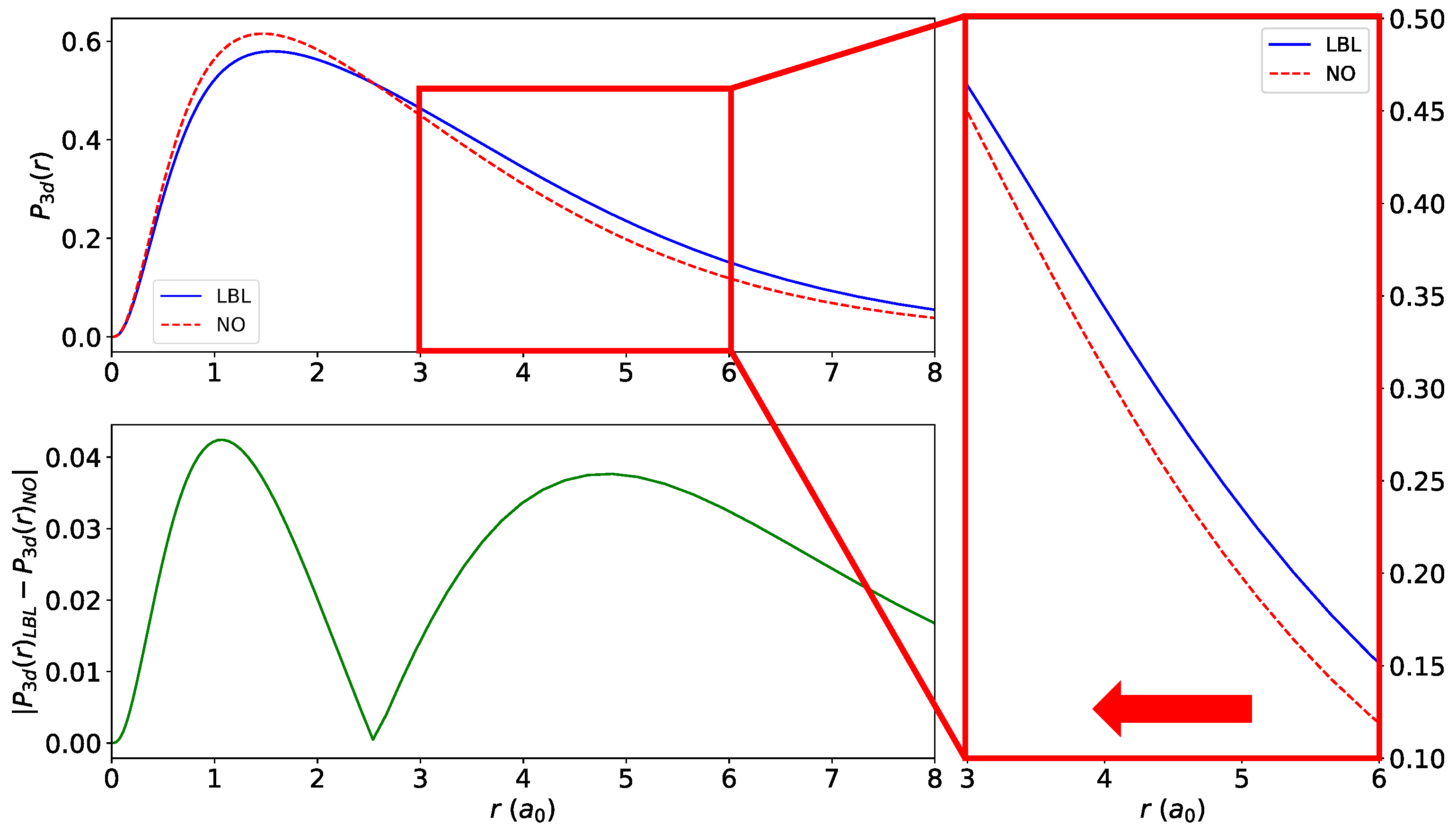
The orbital contraction is more visible in
Figure 3 between 3 and
. The top-left graph shows the large component
of the valence orbital as a function of
r for the LBL calculation (in blue) and the transformed NO (in dashed red) obtained from the S substitution MR calculation. The bottom-left graph shows the absolute difference between these two orbital bases. There are multiple zones where the NO valence orbital is more contracted than the LBL one. On the right-hand side, the
region is magnified, where the contraction is clearly denoted by the red arrow. Even this small contraction (about
in this region) can cause a difference in the
A HFS constants. The same behavior applies for the valence orbitals of the ground and the
P excited levels, as well as in the
B HFS constants.
Table 5.
Comparison of (in ) and (in ) for the levels of 43Ca II between layer-by-layer (LBL) (MCDHF CV ) and natural orbital (NO) calculations. The spectroscopic orbital is highlighted in grey.
Table 5.
Comparison of (in ) and (in ) for the levels of 43Ca II between layer-by-layer (LBL) (MCDHF CV ) and natural orbital (NO) calculations. The spectroscopic orbital is highlighted in grey.
| Subshell | | |
|---|
| LBL | NO | LBL | NO |
|---|
| 2.5227 | 2.3033 | 0.5937 | 0.6947 |
| 2.3718 | 2.3325 | 1.7532 | 1.5547 |
| 2.4586 | 2.9116 | 2.4162 | 1.9883 |
| 2.5629 | 3.0360 | 4.7478 | 5.5875 |
| 3.0079 | 3.1761 | 6.3437 | 7.0810 |
| 2.2484 | 3.8998 | 12.0424 | 5.4211 |
| 5.2031 | 1.8125 | 2.4986 | 23.4276 |
| 1.5182 | 5.1953 | 20.3480 | 6.1427 |
Figure 3.
Comparison between the large valence orbital component of the 43Ca II MCDHF CV SrD LBL calculation in solid blue and multi-reference (MR) with allowed single (S) substitutions from all core orbitals transformed into natural orbitals (NOs) in dashed red (top-left corner). The absolute difference , given in green (bottom-left corner), shows the NO contraction in multiple areas between 0 and . A magnified view is given on the right-hand side; it provides a clearer image of the orbital contraction with the red arrow in the region.
Figure 3.
Comparison between the large valence orbital component of the 43Ca II MCDHF CV SrD LBL calculation in solid blue and multi-reference (MR) with allowed single (S) substitutions from all core orbitals transformed into natural orbitals (NOs) in dashed red (top-left corner). The absolute difference , given in green (bottom-left corner), shows the NO contraction in multiple areas between 0 and . A magnified view is given on the right-hand side; it provides a clearer image of the orbital contraction with the red arrow in the region.
Using the NO basis, we repeated all RCI calculations (labeled NO in
Table 4). The results for both optimizations differ by only a few MHz. We recommend the final NO values, as they account for orbital contraction and show better agreement with experimental values, except for
.
For an accurate theoretical determination of the HFS constants, one should account for the Bohr–Weisskopf (BW) effect [
38], a correction of the finite nuclear magnetization distribution of the nucleus, making a contribution to the HFS. Chakraborty et al. [
30] studied the effect of BW correction on the calculated HFS constants in
43Ca II, with limited correction (at most 0.30% for the
level). The BW-corrected
A HFS constants for the
and
levels are given in
Table 6, but the BW effect could not correct the fact that the values calculated with the LBL orbital basis are closer to the experimental values than the ones calculated with the NO orbitals.
3.2. Ra II
Radium (Ra) is the heaviest alkaline earth metal, with 34 known radioactive isotopes. The most stable,
226Ra, has a half-life of 1600 years [
27]. The isotopes
223Ra and
225Ra, with nuclear spin
and half-lives of
and
days, respectively, only exist in trace amounts. Their short half-lives make experiments challenging, so theoretical hyperfine structure calculations are needed to provide experimental bounds. The levels of interest are the even [Rn]
and [Rn]
levels, as well as the odd [Rn]
levels, for which only a few experimental values are available. Using collinear fast-beam laser spectroscopy, Wendt et al. [
40] determined the HFSs of both
levels, while Neu et al. [
41] studied both the ground
and
levels. Theoretical values were obtained using RCC [
42,
43], Atomic Many-Body Perturbation Theory in the Screened Coulomb Interaction (AMPSCI) [
44], or the relativistic all-order SDpT method [
45]. This is the first paper to compute HFS constants using the MCDHF and RCI methods and to benchmark the new GRASPG [
25] package for high-
Z ions.
With the AS given in
Table 7, the code limited the investigation of orbital substitutions to those no higher than
.
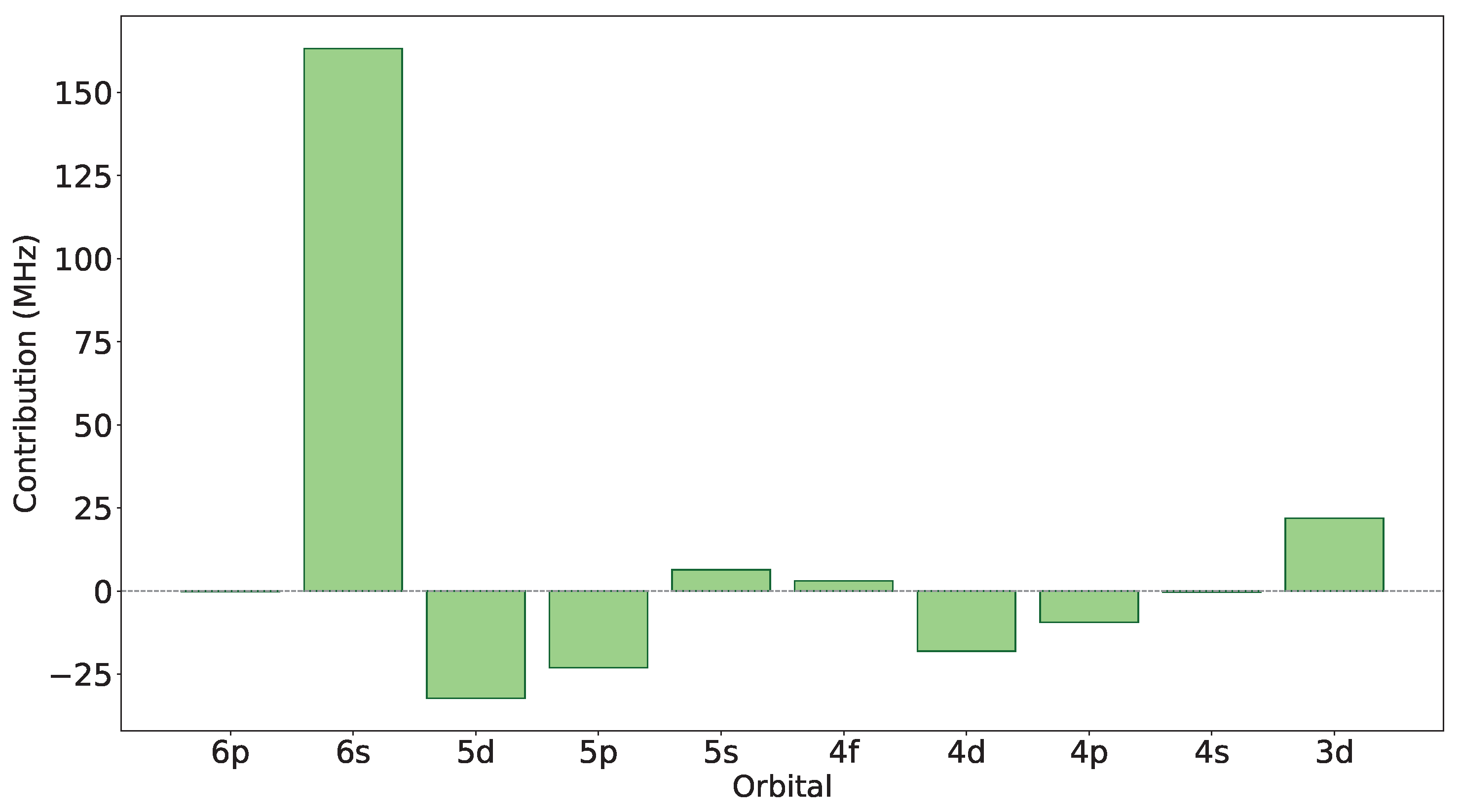
Table 8 and
Figure 4 show that, for the ground level, the highest contribution comes from
substitutions.
and
substitutions can be added to the optimization model in order to follow the Ba/Sr [
15] strategies.
With this understanding, the first MCDHF CV SrD
is already able to give electric quadrupole
A HFS constants that are near the values in the literature, with a maximum difference of
for
. However, more correlations are needed for the magnetic dipole
B constants to be accurately determined, as shown by the discrepancies in the
D levels (
50%). However, when an experimental value exists, the calculated value agrees with only
9% difference for the
constant. Adding deeper correlations with the second MCDHF CV SrD
deteriorates the agreement with the experimental values [
40,
41] and the other theoretical values [
42,
43,
44] for all the
A HFS constants except
. The
B HFS constants are
closer to the calculated theoretical values reported by Sahoo et al. [
42] (RCC). The agreement is preserved for the
constant (
9%) but is now too large compared to the experiment value. We are still convinced that adding correlation orbitals with higher
l encapsulates the orbital polarization that was neglected in the first MCDHF CV SrD
strategy and is important for reliable determination of the
B hyperfine constant [
23].
After the MCDHF calculations, higher-order core–core (CC) correlations are added using RCI. Like in the Ca II case, two models are considered for each optimization strategy by allowing single and double (SD) substitutions. For all
A HFS constants and for each orbital basis, both RCI models (RCI CC SD
and RCI CC SD
) lower the positive values and increase the negative values. However, the added CC correlations are not sufficient to yield a significantly better agreement for the
B HFS constants for the
D levels while using the MCDHF CV SrD
orbital basis. The agreement even worsened for the
level, with nearly a 100 MHz difference with respect to the experimental value. Overall, the best agreement was obtained with the MCDHF CV SrD
+ RCI CC SD
strategy. The agreement between the calculated value and RCC value [
42] is still satisfactory for the
constant.
We recall that, for Sr (Z = 38) and Ba (Z = 56), the
HFS constant was problematic, with an opposite sign between calculated values and those from the literature [
15]. For Ra (Z = 88), the HFS constant does not show the same behavior. To understand this more clearly, we again move to the non-relativistic formalism, where the magnetic dipole HFS constant
A is given as a sum of orbital, spin-dipole, and Fermi contact terms [
46].
Table 9 shows the contribution of the different nonrelativistic hyperfine factors to the total
A constant. For the Hartree–Fock (HF) calculation, the contact term is zero. Adding core–valence (CV) correlations by opening
and
for substitutions to one layer of correlation orbitals
, we see positive interference for the
level and negative interference for the
level. Compared with Sr and Ba, the negative interference between the different terms is less pronounced for Ra, making it less sensitive to neglected higher-order correlation effects derived from triple (T) and quadruple (Q) substitutions, which are the likely cause of the lack of agreement with the experiment for the former elements.
In Ca II, the recommended values for this work were obtained using an NO basis. Following the same approach for Ra II, RCI calculations were repeated, with the results presented in
Table 10. While the LBL orbital basis remains suitable for the ground level, the NO basis provides better agreement for all excited levels, with an outstanding <1% difference with an experimental value of
. Nevertheless, the uncertainty calculation for
encompasses both the NO result and the experimental value.
The Bohr–Weisskopf (BW) effect could significantly affect our HFS
A constants in heavy elements such as radium [
43,
44].
Table 11 reports and compares our BW-corrected values, as determined by using the extracted relative BW corrections reported by Cserveny et al. [
44], with the available theoretical and experimental data. These corrections are more important for the
S and
D states than for the
P states [
44]. It can be seen that our BW-corrected NO values are now closer to the experimental values than our LBL ones, as expected.
Nuclear physicists are also interested in
225Ra. As
strictly implies that
according to the Wigner–Eckart theorem [
23], only the
A hyperfine structure constant can be evaluated for this isotope. Using
223Ra II hyperfine constants in
Table 10, the
225Ra II constants were determined via the HFS electronic constants [
26]:
Table 11 reports the BW-corrected values for the
A HFS constants of
225Ra II, obtained through the use of the extracted relative BW corrections reported by Cserveny et al. [
44], compared with the data from the literature. It shows the overall better agreement of the HFS constants calculated with the transformed NO basis, with the notable exception of the
ground level, where our LBL value is closer to the experimental results. This exception remains unexplained, as it was not the case for
and as these values were calculated using Equation (
23).
Table 11.
Bohr–Weisskopf (BW)-corrected magnetic dipole
A hyperfine structure constants (in MHz) of
223Ra II and
225Ra II
and
, respectively [
39]), determined using the extracted relative BW corrections reported by Cserveny et al. [
44], obtained in this work along with theoretical and experimental data available in the literature. The recommended values are presented in the form of
, with a
confidence level.
a: Th. Sahoo et al. (RCC) [
42];
b: Th. Cserveny et al. (AMPSCI) [
44];
c: Th. Li et al. (RCC) [
43];
d: Th. Pal et al. (SDpT) [
45];
e: Th. Skripnikov et al. (RCC) [
47];
f: Expt. Wendt et al. [
40];
g: Expt. Neu et al. [
41].
Table 11.
Bohr–Weisskopf (BW)-corrected magnetic dipole
A hyperfine structure constants (in MHz) of
223Ra II and
225Ra II
and
, respectively [
39]), determined using the extracted relative BW corrections reported by Cserveny et al. [
44], obtained in this work along with theoretical and experimental data available in the literature. The recommended values are presented in the form of
, with a
confidence level.
a: Th. Sahoo et al. (RCC) [
42];
b: Th. Cserveny et al. (AMPSCI) [
44];
c: Th. Li et al. (RCC) [
43];
d: Th. Pal et al. (SDpT) [
45];
e: Th. Skripnikov et al. (RCC) [
47];
f: Expt. Wendt et al. [
40];
g: Expt. Neu et al. [
41].
| Reference | | | | | |
|---|
| 223Ra II |
|---|
| This work (LBL) | 3329 ± 359 | 68 ± 15 | −21 ± 4 | 603 ± 63 | 52 ± 4 |
| This work (NO) | 3451 ± 331 | 72 ± 18 | −24 ± 4 | 640 ± 61 | 55 ± 3 |
| Th. a | 3567 | 77 | −24 | | |
| Th. b | 3424 ± 71 | 95 ± 20 | −29 ± 10 | 675 ± 13 | 57.7 ± 60 |
| Th. c | 3426 ± 82 | 79.9 ± 1.7 | ± 2.3 | 660 ± 11.4 | 56.5 ± 1.2 |
| Th. d | 3450 | 80 | −24 | 672 | 54 |
| Expt. f | 3398.3 ± 2.9 | | | 667 ± 2.1 | |
| Expt. g | 3404 ± 1.9 | | | | 56.5 ± 8 |
| | 225Ra II |
| This work (LBL) | −27,424 ± 3038 | −560 ± 110 | 158 ± 37 | −4984 ± 534 | −442 ± 24 |
| This work (NO) | −29,233 ± 4193 | −612 ± 144 | 166 ± 37 | −5478 ± 823 | −487 ± 59 |
| Th. a | −28,978 | −626 | 194 | | |
| Th. e | −27,731 | | | −5451 | −461 |
| Expt. f | | | | −5446 ± 7 | |
| Expt. g | −27,731 ± 13 | | | | −466.4 ± 4.6 |
3.3. Ra I
Neutral radium (Ra I) has two valence electrons. Only a few levels have had their HFSs experimentally studied. The odd [Rn]
was studied by Lynch et al. [
48] at the ISOLDE facility, and [Rn]
,
1 were studied by Wendt et al. [
40]. The HFSs of the even [Rn]
,
3 levels are only known theoretically. Hassouneh et al. [
49] and Bieroń et al. [
50] studied them using the MCDHF method, while Dzuba et al. [
51] used a Relativistic Hartree–Fock + Configuration Interaction (RHF + CI) method to determine the HFS of
213Ra I
. Their values were used to compute the HFS constants for
225Ra II using Equation (
23). The latter two were computationally limited by the number of CSFs or by using a pseudo-relativistic Schrödinger Hamiltonian that would not be sufficient for studying the intense relativistic effects of electrons in heavy atoms.
Nezosi et al.’s [
15] Ba I HFS study highlighted that a multi-reference (MR) is needed for heavy neutral elements such as Ra I when using the MCDHF method. As the main goal of this paper is mainly to transpose Sr II/Ba I–II MCDHF strategies, the configuration that interacts the most with the reference is added for both studied parities. The even [Rn]
,
3 levels were augmented by a [Rn]
configuration, while the odd [Rn]
,
1 levels were augmented by a [Rn]
configuration. Seven correlation layers were considered, as shown in
Table 12, for the optimization of the MR formed by the two parity configurations.
The first calculations were performed using the layer-by-layer (LBL) approach, and the results are displayed in
Table 13. Due to the two-valence-electron structure of Ra I, an additional optimization strategy could be considered based on valence–valence (VV) correlations. Computations showed that the MCDHF VV SrD optimization strategy is not sufficient to account for the core polarization needed for an accurate determination of the hyperfine structure, with differences ranging from
40 MHz for
to
260 MHz for
. Adding core–valence (CV) correlations in the MCDHF VV SrD + CV SrD
strategy adds the important polarization of the core caused by the valence electrons with already satisfactory agreement with values from the literature for the
A constants. The cost of including these important correlations is an increase in the number of CSFs by nearly 70-fold for the even levels and 100-fold for the odd levels. One final layer of optimization in MCDHF VV SrD + CV SrD
was added to match the Ba I [
15] model. It again shows that the more correlations there are, the better the outcome, especially for the
B hyperfine constants, when asymmetrical
d (
) core orbital substitutions are allowed. This behavior was already observed in Ba, and it reinforces the idea that substitutions from orbitals with a higher
l take into account the orbital polarization that was previously neglected and are therefore important for reliable determination of
B [
23]. This third layer of optimization increases the HFS constants for all the levels in terms of the absolute values.
Adding higher-order correlations with SD substitutions in an RCI step greatly increases the number of CSFs to a total of 2,933,035 for the biggest MCDHF VV SrD + CV SrD
+ RCI CC SD
step. Therefore, even if T substitutions are known, in Na I, to correct CC correlations with the HFS [
21], they could not be added in Ra I. Nevertheless, the largest model shows the best agreement for this approach, with a discrepancy of only 1 MHz for
, but can still under-perform for
or
, with
60 and
20% differences with respect to values from the literature, respectively.
Taking the LBL picture as a whole when determining the final values in the
format yields satisfactory results for
, with an only
difference with respect to the latest available MCDHF values [
49]. Our calculations are in agreement with the available experimental value for
[
40], with an
2% discrepancy, and outperform Hassouneh et al.’s [
49] MCDHF calculations for this level while giving an uncertainty estimation.
Moving to the NO basis allows us to attain overall better agreement than the LBL calculation, as was already the case for 43Ca II and 223Ra II. The final values with uncertainty estimates cover other theoretical calculations. When the NO basis degrades the values relative to the LBL basis, it is always only by a few percentage points.
Using the correction factor reported by Bieroń [
50], our results for
223Ra I in
Table 13 now include the BW effect. A rescaling of the
A hyperfine constants using Equation (
23) for
225Ra I was also done. The corrected results are shown in
Table 14. The situation is less clear than in the case of Ra II. There is no evidence of a quasi-systematic improvement in the agreement with the measurements when one transforms LBL orbitals into NO orbitals. Now, one can see from
Table 14 that the BW-corrected MCDHF-RCI calculations reported by both Hassouneh and Salah [
49] and Bieroń [
50] show better general agreement with experimental results than our BW-corrected values. There are still two exceptions: the
level in
223Ra I and the
level in
225Ra I. For these levels, our BW-corrected NO and LBL HFS
A constants are in better agreement with the measurements reported by Wendt et al. [
40] and Guest et al. [
52], respectively. This shows that the differences seen here in Ra I are more due to the correlation model adopted than the BW effect. However, this BW correction factor (
0.96) reported by Bieroń [
50], when applied to each level, is a limited approach, as [
30,
43,
44] showed the dependence of the BW effect on the level studied.
Table 13.
Magnetic dipole
A and electric quadrupole
B hyperfine structure constants (in MHz) of
[
39]) compared to available theoretical and experimental data. The recommended values are given in the form of
, exhibiting a
confidence level.
★: Number of CSFs obtained after reduction using the rcsfginteract_csfg code;
a: Th. Hassouneh et al. (MCDHF) [
49];
b: Th. Bieroń et al. (MCDHF) [
50];
c: Th. Calculated from Dzuba et al. (RHF + RCI) [
51];
d: Expt. Lynch et al. [
48];
e: Expt. Wendt et al. [
40].
Table 13.
Magnetic dipole
A and electric quadrupole
B hyperfine structure constants (in MHz) of
[
39]) compared to available theoretical and experimental data. The recommended values are given in the form of
, exhibiting a
confidence level.
★: Number of CSFs obtained after reduction using the rcsfginteract_csfg code;
a: Th. Hassouneh et al. (MCDHF) [
49];
b: Th. Bieroń et al. (MCDHF) [
50];
c: Th. Calculated from Dzuba et al. (RHF + RCI) [
51];
d: Expt. Lynch et al. [
48];
e: Expt. Wendt et al. [
40].
| Strategy | | | | | | | |
|---|
| | | | | | | | | | | | | | | | | | |
|---|
| | Layer-by-layer (LBL) |
| MCDHF VV SrD | 626 | −458 | 91 | 910 | 292 | 135 | −81 | 303 | 898 | 350 | 199 | 635 | 896 | −323 | −225 | 228 | 852 | 565 | 425 |
| RCI CC SD | 85,320 ★ | −559 | 78 | 266,206 ★ | 272 | 133 | −75 | 272 | 189,081 ★ | 382 | 211 | 172,279 ★ | 963 | −322 | −219 | 353 | 320,622 ★ | 637 | 447 |
| RCI CC SD | 170,014 ★ | −567 | 98 | 531,502 ★ | 273 | 162 | −73 | 320 | 377,264 ★ | 388 | 264 | 353,923 ★ | 976 | −327 | −220 | 375 | 640,392 ★ | 646 | 459 |
| MCDHF VV SrD + CV SrD | 41,956 | −596 | 70 | 59,801 | 367 | 127 | −136 | 285 | 65,843 | 425 | 188 | 64,276 | 1221 | −421 | −362 | 395 | 91,187 | 717 | 625 |
| RCI CC SD | 123,653 ★ | −572 | 79 | 322,284 ★ | 320 | 134 | −100 | 250 | 248,578 ★ | 404 | 209 | 237,283 ★ | 1059 | −344 | −274 | 347 | 404,447 ★ | 666 | 477 |
| RCI CC SD | 208,347 ★ | −583 | 101 | 587,580 ★ | 320 | 166 | −98 | 302 | 436,761 ★ | 410 | 267 | 413,927 ★ | 1070 | −345 | −274 | 371 | 724,217 ★ | 675 | 483 |
| MCDHF VV SrD + CV SrD | 116,496 | −658 | 129 | 167,242 | 421 | 212 | 212 | 396 | 186,546 | 477 | 328 | 177,207 | 1385 | −477 | −416 | 464 | 253,427 | 805 | 719 |
| RCI CC SD | 197,118 ★ | −623 | 129 | 429,417 ★ | 364 | 206 | −116 | 357 | 355,757 ★ | 447 | 330 | 349,045 ★ | 1180 | −389 | −311 | 404 | 563,936 ★ | 735 | 548 |
| RCI CC SD | 280,602 ★ | −628 | 129 | 693,084 ★ | 362 | 204 | −113 | 343 | 553,300 ★ | 449 | 330 | 524,247 ★ | 1179 | −372 | −309 | 397 | 881,802 ★ | 738 | 523 |
| | Natural orbitals (NOs) |
| MCDHF VV SrD | 626 | −458 | 91 | 910 | 292 | 135 | −81 | 303 | 898 | 350 | 199 | 635 | 896 | −323 | −225 | 228 | 852 | 565 | 425 |
| RCI CC SD | 85,320 ★ | −581 | 77 | 266,206 ★ | 280 | 134 | −76 | 278 | 189,081 ★ | 398 | 210 | 172,279 ★ | 1000 | −384 | −202 | 444 | 320,622 ★ | 657 | 554 |
| RCI CC SD | 170,014 ★ | −607 | 112 | 531,502 ★ | 291 | 184 | −79 | 369 | 377,264 ★ | 416 | 298 | 353,923 ★ | 1048 | −407 | −208 | 480 | 640,392 ★ | 691 | 600 |
| MCDHF VV SrD + CV SrD | 41,956 | −599 | 72 | 59,801 | 369 | 129 | −135 | 290 | 65,843 | 427 | 192 | 64,276 | 1216 | −429 | −353 | 410 | 91,187 | 714 | 639 |
| RCI CC SD | 123,653 ★ | −595 | 80 | 322,284 ★ | 331 | 136 | −104 | 257 | 248,578 ★ | 420 | 212 | 237,283 ★ | 1093 | −400 | −256 | 422 | 404,447 ★ | 686 | 569 |
| RCI CC SD | 208,347 ★ | −621 | 117 | 587,580 ★ | 342 | 189 | −107 | 354 | 436,761 ★ | 437 | 305 | 413,927 ★ | 1138 | −421 | −262 | 480 | 724,217 ★ | 718 | 613 |
| MCDHF VV SrD + CV SrD | 116,496 | −664 | 132 | 167,242 | 425 | 216 | −157 | 403 | 186,546 | 481 | 334 | 177,207 | 1377 | −492 | −400 | 494 | 253,427 | 800 | 746 |
| RCI CC SD | 197,118 ★ | −638 | 147 | 429,417 ★ | 374 | 231 | −119 | 409 | 355,757 ★ | 459 | 370 | 349,045 ★ | 1202 | −458 | −284 | 505 | 563,936 ★ | 748 | 668 |
| RCI CC SD | 280,602 ★ | −662 | 147 | 693,084 ★ | 385 | 231 | −123 | 400 | 553,300 ★ | 474 | 370 | 524,247 ★ | 1237 | −450 | −292 | 506 | 881,802 ★ | 776 | 658 |
| This work (LBL) | −593 ± 63 | 109 ± 35 | | 318 ± 89 | 177 ± 46 | −95 ± 40 | 322 ± 41 | | 416 ± 62 | 287 ± 74 | | 1075 ± 203 | −348 ± 45 | −267 ± 89 | 381 ± 28 | | 686 ± 94 | 488 ± 65 |
| This work (NO), recommended | −630 ± 57 | 125 ± 38 | | 339 ± 94 | 201 ± 52 | −103 ± 45 | 374 ± 47 | | 442 ± 59 | 324 ± 79 | | 1141 ± 189 | −426 ± 44 | −254 ± 85 | 489 ± 29 | | 728 ± 87 | 624 ± 61 |
| Th. a | −607 | 130 | | 218 | 213 | −143 | 388 | | 428 | 346 | | 1207 | −468 | −341 | 419 | | 622 | 655 |
| Th. b | −612 | 125 | | 382 | 210 | −140 | 382 | | 428 | 346 | | 1252 | −476 | −330 | 419 | | | |
| Th. c | −604 | | | 257 | | −47 | | | 403 | | | 1185 | | −242.3 | | | | |
| Expt. d | | | | | | | | | | | | 1202.5 ± 3.0 | −472.1 ± 2.0 | | | | | |
| Expt. e | | | | | | | | | | | | 1202.1 ± 0.6 | −470.2 ± 1.2 | −344.5 ± 0.9 | 421.5 ± 1.6 | | 699.6 ± 3.3 | 688.5 ± 4.0 |