Abstract
Lithium (Li)-rich continental brines found in the Lithium Triangle region in South America are a natural resource of paramount importance. In the present research, the analytical performance of laser-induced breakdown spectroscopy (LIBS) technology was assessed for the quantitative analysis of Li in natural brines aimed at enhancing the efficient exploration of salt flats (called salars). Brine samples were collected from different salars located in the Puna plateau (Northwest Argentina) and analyzed by LIBS in the form of solid pressed pellets. Broadband emission spectra (180–900 nm) were recorded and spectrally analyzed by specially designed computational algorithms. The laser-induced plasmas were characterized by calculating the electron density and the temperature. The Li elemental concentrations in the brines were determined through univariate calibration with the Li I emission line at 670.77 nm by using a suitable set of standards with Li concentrations up to 1300 µg/g. The calculated limit of detection was LoD = 0.2 ± 0.1 µg/g. The Li content in the brines determined with LIBS showed a good agreement (normalized standard deviation: σN = 25%) with the concentrations measured with atomic absorption spectroscopy. The results demonstrated the feasibility of the LIBS technique for the quantitative analysis of Li in natural brines, thus contributing to advancing the exploration of Li-rich resources.
1. Introduction
In the last decade, lithium (Li) has emerged as a strategic element mainly due to the fast-growing demand of Li salts for the battery industry (i.e., computers, phones, and electric/hybrid vehicles), as well as for the storage of green energy (i.e., solar, wind, and waves) [1]. Nowadays, 58% of the global Li resources are contained in continental brines from salt flats (locally known as salars) and, in a minor extent, within granite pegmatite deposits (i.e., spodumene and petalite ores), seawaters, and geothermal waters [2]. Continental brines are highly saline solutions containing large quantities of Na together with variable contents of Li and other minor elements, including K, Mg, Ca, Sr, Ba, Rb, and Cs. In South America, Argentina, Bolivia, and Chile constitute the so-called Lithium Triangle, an extensive region where numerous salars with Li-rich brines are found [3]. All together, these salars account for about 80% of the Li resources in brines worldwide. The major deposit of Li in Argentina is located in the Puna region (a high-altitude plateau with an average elevation of 3600 m.a.s.l.) within the provinces of Jujuy, Salta, and Catamarca, occupying the third place of the overall world Li production from brines [4]. Salars have distinctive geological characteristics; consequently, the Li concentration in the brines varies spatially in each salar, ranging on average from 10 to 1000 µg/g [1,3]. However, reliable data about the availability of raw materials in salars, i.e., Li salt concentrations, are still quite limited. As outlined in the recent review by López Steinmetz et al. [5], a better knowledge of the Andean salars and their Li endowment is essential to carry out a feasible, integral, and efficient exploration to recover the resource while avoiding, minimizing, or remediating potential adverse effects. In fact, the unplanned mining of salars may have negative side effects on the ecosystem and the human population in the region. Consequently, national policies have been triggered by local governments to protect the resource and foster the development of new disruptive technologies for sustainable Li exploitation [6].
Among laser-based technologies, laser-induced breakdown spectroscopy (LIBS) is a useful analytical tool which is very attractive to complement the conventional techniques currently in use for Li determination in brines, such as atomic absorption spectroscopy (AAS) and inductively coupled plasma–atomic emission spectroscopy (ICP–AES) [7]. LIBS is based on the spectral measurement of the radiation emitted by a plasma generated from the laser-ablated target material, which emits characteristic spectral lines in the UV–Vis spectral range (200–900 nm). Due to its inherent features of simplicity and versatility, LIBS has the capacity to accomplish rapid, in situ, multi-element measurements requiring a minimum sample treatment [8]. Furthermore, it is able to detect light elements, i.e., Li, which are hardly detected by other analytical methods [9]. LIBS is a very active field of research worldwide, with a widespread range of applications [10]. The usual approach to accomplish quantitative LIBS analysis relies on the construction of calibration curves employing matrix-matched standards under the assumption of a homogeneous plasma in local thermodynamic equilibrium (LTE) [11]. Nevertheless, those standards are often limited or unavailable for geological and environmental targets due to the occurrence of non-negligible matrix effects [12].
Regarding geochemical studies, LIBS has been mainly applied to the analysis of Li in different geological matrices, such as rocks and minerals, e.g., muscovite and other Li-bearing minerals [13,14]. On the other hand, the application of the LIBS technique for the elemental characterization of Li content in brines has been poorly explored. This is mainly due to the well-known drawbacks (i.e., splashing, bubbles, surface ripples, and lower emitted intensity) of LIBS analysis of liquid samples, such as brines, which worsen its analytical performance in comparison to solid samples [15]. To overcome these issues, different approaches have been reported [16,17,18]. Erbetta et al. [19] analyzed natural brines extracted from the Atacama Desert in Chile (0.5–1.75% wt. Li) by using a handheld LIBS system. Xing et al. [20] reported the quantitative analysis of natural brines (5–40 µg/g Li) achieved via the combination of LIBS and Convolutional Neural Network (CNN). In the latter, the authors mentioned matrix effects as a main factor affecting the measurements. In both studies, the potentialities of LIBS for the quantitative analysis of brines measured as sprays and featuring Li concentrations at either very low (trace) or high levels (%wt.) were clearly evidenced. Nevertheless, many Li-rich salars usually present intermediate concentrations of ~1000 µg/g Li [3].
In this context, more research is still needed to further extend the LIBS analytical range for Li determination, as well as minimizing the matrix effects usually present in the analysis of environmental samples. In a previous study by our group, it was shown that the approach of sample preparation in the form of pressed pellets from pure calcium hydroxide produced suitable quantitative results, minimizing possible matrix effects [21]. Even though the solid pellets required some minimum preparation, which prevents onsite analysis, this procedure is commonly used since it matches the inherent advantages of solid targets, together with simplicity, a low cost, repeatability, and sensitivity to trace monitoring of liquid environmental samples. In later works, this method was successfully applied for the elemental analysis of different elements of interest [22,23,24,25]. In the present work, the analytical capability of the LIBS technique for the determination of Li in brines was further extended and assessed by analyzing natural samples collected from different salars of the Lithium Triangle. The analytical procedure was carried out by specially designed algorithms which conducted the pre-treatment of the recorded data, spectral analysis, plasma characterization, and the determination of the Li elemental concentration by univariate external calibration with a suitable set of standard samples. Moreover, the analytical performance of the LIBS technique was evaluated by comparing the obtained results with the conventional AAS technique.
2. Materials and Methods
2.1. Samples
The samples employed in this study were brines collected from ponds or mechanically dug exploration test pits within different salars located in the Puna region of Argentina. The collected samples were stored in pre-cleaned 10 mL plastic bottles, avoiding the inclusion of salts or sediments. The analytical set was composed of 11 samples (i.e., #1–#11; 12 mL volume), which were transported to the laboratory for subsequent analysis by LIBS and AAS techniques. The AAS measurements were performed following standard procedures described in Reference [26]. For LIBS analysis, the samples were prepared in pressed pellets from pure calcium oxide (CaO, Aldrich Powder 98%) in powder form, as reported previously [21]. Each pellet was prepared by mixing the brines with 6 g of CaO. The mixture was stirred well in such a way that the elements resulted in being uniformly distributed inside the solid matrix; dried in an oven (at 70 °C) until constant weight was attained; finely grinded; and pressed in a steel die at ≈10 ton/cm2 for about 10 s to form pellets of approximately 3 cm in diameter, 1 cm in thickness, and 8 g in weight. Following the same procedure, 11 reference samples were manufactured for calibration purposes by using standard solutions with Li concentrations in the range of 0–1300 µg/g. The Li standard solutions were prepared by diluting a stock solution (lithium carbonate, Li2CO3, provided by Agilent) with appropriate volumes of doubly distilled water (σ < 5 μS/cm). In addition, a blank sample was included.
2.2. LIBS Measurements and Analysis
The LIBS equipment employed for Li analysis in brines is shown in Figure 1. A Q-switched Nd: YAG laser (CNI Tech. Co., Ltd., Seoul, Republic of Korea, model DPS–1064–BS–DD, wavelength 1064 nm, pulse width 9 ns, pulse energy 20 mJ, repetition rate 25 Hz) was focused on right angles to the sample surface to generate the plasmas in air at atmospheric pressure. The focusing lens (100 mm focal length) was placed at a distance of 95 mm from the sample surface. The estimated incident laser irradiance on the sample surface was about 10 GW/cm2. During the measurements, the samples rotated at 500 rev min–1 to avoid the formation of a deep crater due to delivering too many laser shots at the same point. A plastic nozzle of 4 mm in diameter was used to blow air over the ablation area (pressure < 1 psi) to get rid of the dust released by laser shots, thus avoiding the spark of the breakdown in the air above the samples’ surface and improving the repeatability of the measurements. The whole plasma emission was collected using fiber optics (100 μm core diameter) placed at a 5 mm distance from the laser spot on the target at a 45-degree angle and transmitted to the entrance of an eight-channel spectrometer (Avantes, Apeldoorn, The Netherlands, model AvaSpec–ULS2048–USB2) equipped with a charge-coupled device (CCD) with a total spectral range from 180 to 888 nm and a spectral resolution from 0.6 nm to 0.22 nm. The LIBS spectra were acquired with a delay of 1.04 μs and an integration time of 1.05 ms in such a way that the initial continuous background, mainly caused by bremsstrahlung radiation, was minimized. After that, the plasma emission during its entire lifetime was recorded. To reduce the statistical error and to improve the signal-to-noise ratio, each measurement was replicated at 5 different positions in the samples. On each position, the recorded spectrum was the result of the in-software accumulation of individual spectra generated from 100 consecutive laser shots after discarding 250 cleaning shots.
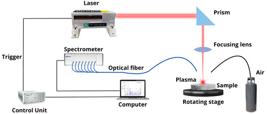
Figure 1.
Experimental LIBS setup.
After the acquisition, the raw spectral data (i.e., 1024 pixels vs. emission intensity) were pre-processed in software. Specifically, this initial data processing comprised automated routines for wavelength calibration, removal of the “dark” background (i.e., non-laser-induced spectrum), and correction by the spectral efficiency of the optical system, as explained in the following. Wavelength calibration was carried out by recording the spectrum of a standard Hg pencil lamp to establish a pixel-to-wavelength relationship which was applied to the X-axis of all spectra. The dark background was measured under the same spectrometer settings but without laser firing, and it was subtracted from the intensities of all wavelengths in the spectra. The spectral efficiency was measured using calibrated standard deuterium and tungsten lamps (Avalight from Avantes) and applied to the Y-axis of the spectra. To validate the analytical results of LIBS, the Li concentrations in natural brine solutions were also determined by AAS (Shimadzu AA700) in triplicate by diluting with ultrapure water (Milli-Q®) and further averaged.
3. Results and Discussion
In this section, we describe the processing and spectral analysis of the recorded data (Section 3.1), the plasma characterization (Section 3.2), and the quantitative analysis of Li in the natural brine samples, together with the evaluation of its accuracy (Section 3.3).
3.1. Processing and Spectral Analysis
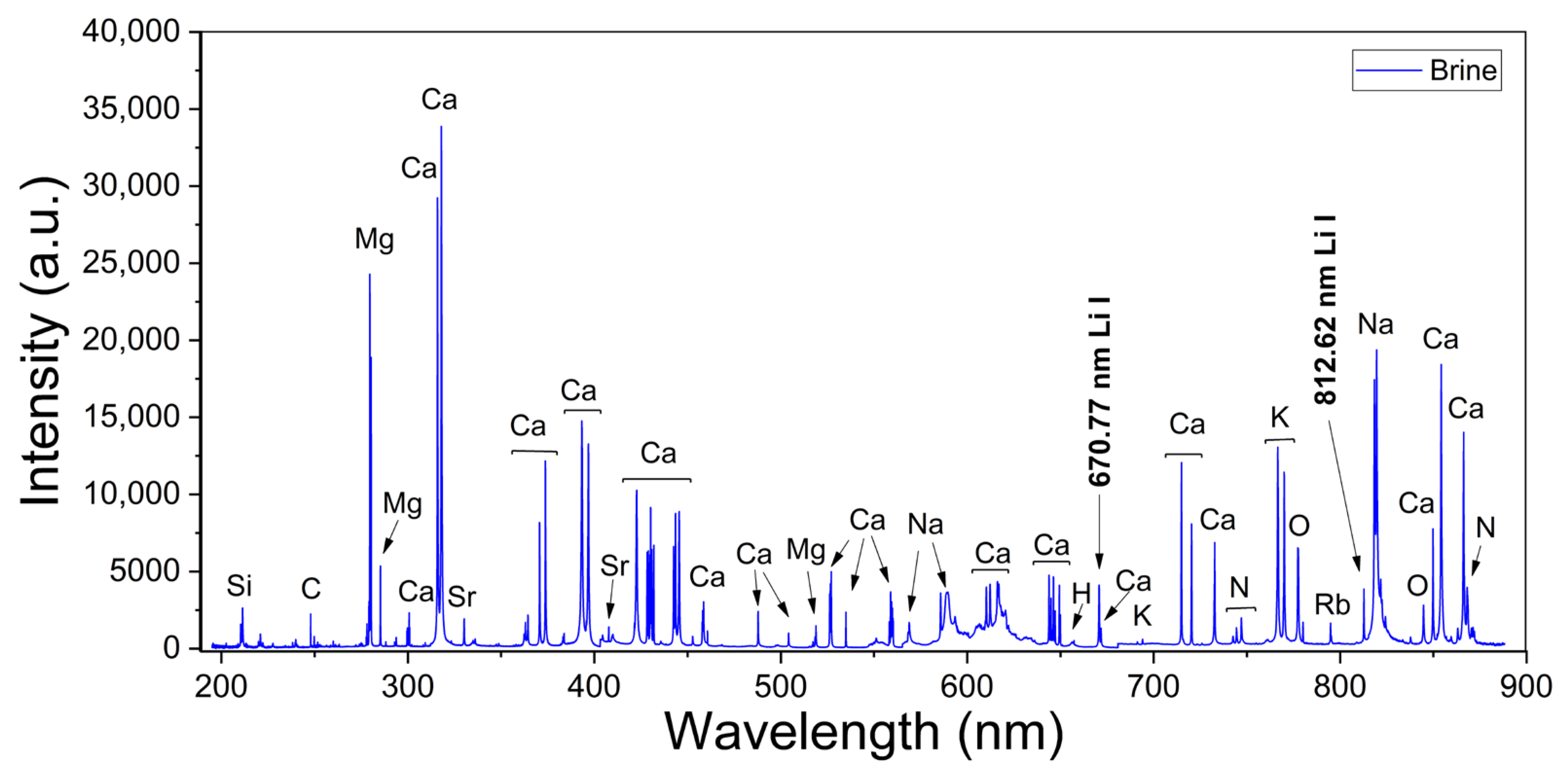
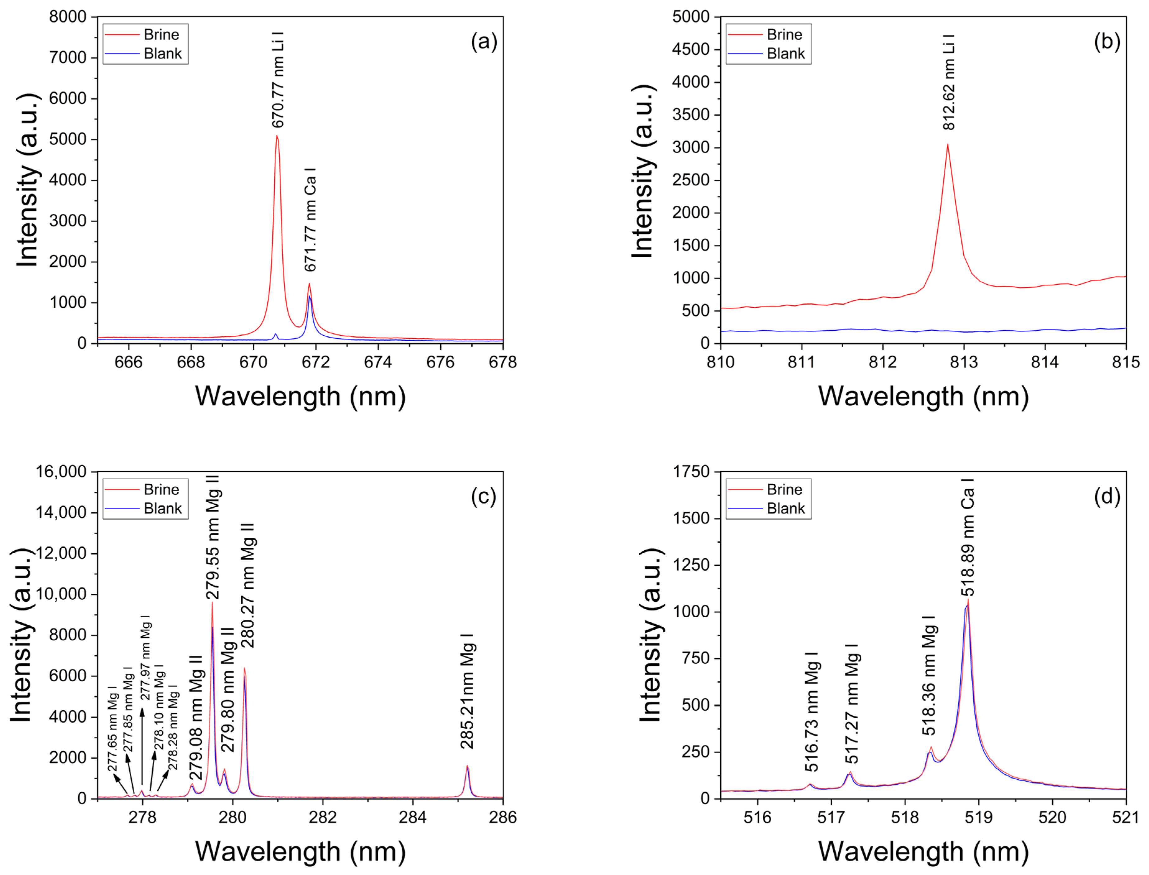
Broadband LIBS spectra were measured from both calibration and analytical brine samples. A typical spectrum recorded from brines is shown in Figure 2, where the main emission lines for the detected elements are indicated. The spectral lines measured for each element corresponded to transitions belonging to neutral atomic and singly ionized species which were identified with the atomic data from the NIST Atomic Spectra Database [27]. The spectra show intense emission peaks of Ca and Na, which are the major elements of the sample matrix and the brines, respectively, as well as several weaker peaks from Li, C, Mg, K, Si, and Rb that are present in the brines at a trace level. In addition, peaks from H, N, O, and Sr are detected due to contributions of both the surrounding ambient air excited by the plasma plume and the sample’s matrix. In our experimental conditions, the measured spectral lines of Li I, Ca I, Mg I–II, and H I were used for quantification and characterization of the plasmas (Table 1). Two Li I spectral lines were measured at 670.77 nm (Figure 3a) and at 812.62 nm (Figure 3b) from all the samples with different emission intensities related to their Li concentrations. The adjacent Ca I spectral line at 671.77 nm was used for normalization purposes. A selected set of Mg I–II lines and the Hα line was used for plasma characterization. The recorded spectral lines were isolated, free from spectral interference of other emission lines, and had suitable SNR. The analysis of the spectra was carried out by computational algorithms specially designed in MATLAB R2024b® and Python 3.13.1® environments. The algorithms comprised routines for (i) fitting of line profiles, (ii) plasma characterization, and (iii) quantitative analysis of the Li content in the analyzed brines.
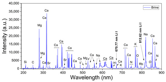
Figure 2.
Broadband LIBS spectrum from brines (sample #11). The main detected peaks, including Li, are indicated.
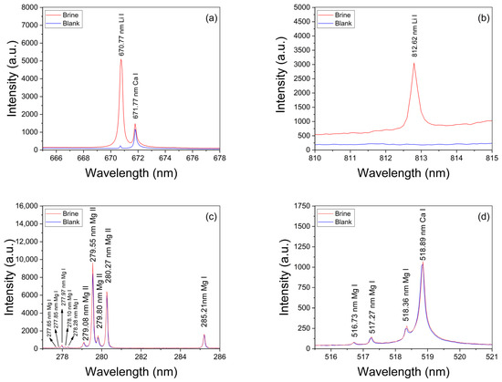
Figure 3.
Spectral lines of Li I measured in brines (sample #11) at (a) 670.77 nm and (b) at 812.62 nm. Ca I line at 671.77 nm was used for normalization. (c,d) Mg I–II emission lines used for calculation of the plasma temperature via the Saha–Boltzmann plot. The spectrum from the blank is also included for comparison.
The Doppler broadening estimated for a typical range of plasma temperatures (i.e., kT = 1 eV) was lower than wD ≈ 0.05 nm, whilst the estimated instrument broadening was wInstr ≈ 0.16 nm. Hence, taking into account the typical values for the electron density achieved in LIBS experiments (Ne~1017 cm−3), the dominant broadening mechanisms that determined the observed line shapes were due to both the instrument and the Stark effect [28]. The estimated instrument broadening was wInstr ≈ 0.16 nm. Non-hydrogenic lines from neutral atoms and ions (quadratic Stark effect) have Stark widths typically less than 0.01 nm. Conversely, the Hα line (linear Stark effect) presents a considerably larger Stark width, typically ≥1 nm. For these reasons, the line shapes of Li, Ca, and Mg transitions were dominated by the instrumental broadening, while the Hα line profile was mainly given by the Stark broadening and, thus, it was employed for the calculation for the electron density of the plasma.
The line intensities were obtained from the spectra (pre-processed) by fitting the measured peaks with a Lorentzian function (mainly due to the instrumental profile) to obtain their net intensities given by the integrated areas of the line profiles with background discount. For each sample, the net intensities of the elements of interest (i.e., Mg, H, Ca, and Li) were averaged over the different measurement positions, and the associated errors corresponded to the standard deviation of the mean values. Moreover, the coefficients of variation (CVs) were calculated as the relative standard deviations (i.e., standard deviation over mean value expressed as a percentage).
3.2. Plama Characterization
The laser-induced plasma was characterized through the determination of the temperature and the electron density, assuming that it was homogeneous and close to LTE conditions [11]. The latter is generally fulfilled in LIBS experiments by the relatively high electron densities achieved (~1017 cm–3), which is above the critical value required by McWhirter’s criterion [29]. McWhirter’s criterion is necessary for but not sufficient to assure LTE. The plasma electron density was measured from the Stark broadening of the Balmer Hα line (at λ = 656.30 nm) by using the diagnosis tables of Gigosos and Cardeñoso [30], thus providing the electron density (Ne [m–3]) as a function of the Stark width (wStark [nm]) of the Balmer series. Namely,
Self-absorption of a spectral line is governed by its optical thickness (τλ), which reaches its maximum value at the line center (λ0) [31]. As investigated in our previous works [22,32], given the large Stark broadening of the Hα line, self-absorption tends to spread out toward the line wings at the expense of the line center; thus, τλ0 decreases at the line center, making it sufficiently too low (i.e., τλ0 << 1) to consider the self-absorption of the line negligible.
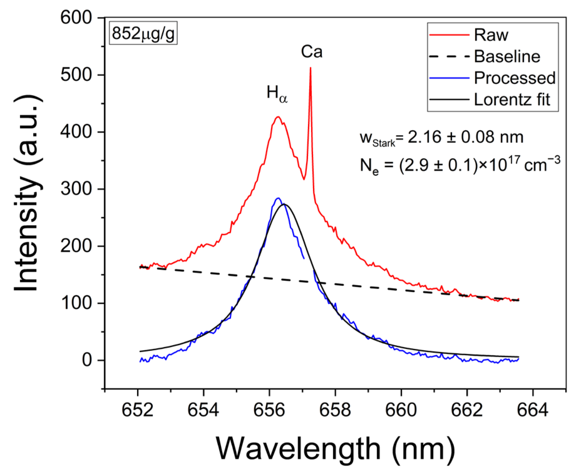
The experimental Hα profiles were fitted with a Lorentzian function related to its Stark broadening. The Stark widths obtained were in the range of wStark = 2.0–2.2 nm, making them compatible with the values reported in other works [33,34]. An example of such a fitting is shown in Figure 4. Despite the fact that it is observed that the Hα profile is weakly interfered by a Ca I line at 657.28 nm, the contribution of this peak did not affect the fitting, and it was removed by the algorithm. After the electron density was calculated, the temperature was determined from the Saha–Boltzmann plot. The Saha–Boltzmann plot was constructed with a set of 10 Mg I–II selected spectral lines (Figure 3c,d), with energy levels in the range of 4.422–8.864 eV, and reported transition probabilities (Table 1) [27]. Mg was selected since it was present at a trace level, and then self-absorption is expected to be not important, as shown below. On the other hand, the use of the measured Ca I–II spectral lines was discarded because of the high Ca content of the sample’s matrix, which will cause a significant self-absorption of its emission lines.
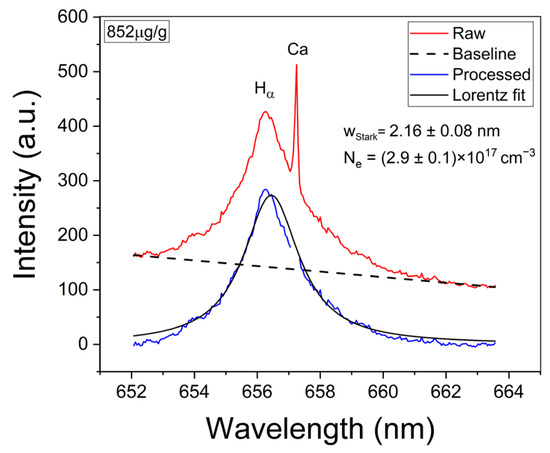
Figure 4.
Example of analysis of the Hα spectral line. The obtained values for wStark and the calculated electron density (Ne) are shown (sample: Reference Li 852 µg/g).
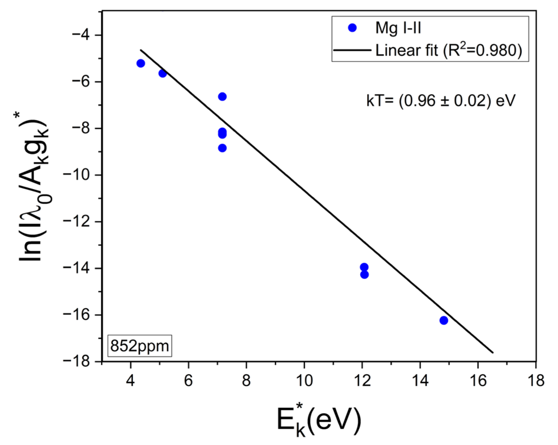
To evaluate a possible self-absorption of the measured Mg I–II emission lines, the experimental ratios of the resonant lines 279.55 Mg II and 280.27 Mg II, which belong to the same multiplet, were compared with the corresponding theoretical intensity ratio expected for an optically thin plasma. Namely, I2795.5/I2802.7 = (Aji2795.5 gj2795.5)/(Aji2802.7 gj2802.7) ≈ 2. In this way, a reduction in the experimental ratio would be indicative of self-absorption. Conversely, if the ratio remains approximately constant, then self-absorption is negligible [23,35]. The mean experimental ratio calculated for all the samples was 1.52 ± 0.03, where the associated error was the standard deviation. It was deduced that self-absorption of these Mg II lines was low to moderate in our experiment and, consequently, also for the other less intense Mg I-II spectral lines of Table 1, being suitable for plasma characterization. An example of an obtained Saha–Boltzmann plot is shown in Figure 5, where the plasma temperature deduced from the slope of the linear regression is indicated. For all the analyzed samples (i.e., calibration and brines), the obtained mean values for the electron density and the temperature were Ne = (2.8 ± 0.1) × 1017 cm–3 and kT = (0.88 ± 0.01) eV, respectively. The errors corresponded to the standard deviations of the mean values.

Figure 5.
Example of Saha–Boltzmann plot constructed with Mg I–II lines of Table 1. The calculated temperature (kT) is shown (sample: reference Li 852 µg/g).
The calculated minimum electron number density necessary to satisfy LTE conditions following McWhirter’s criterion was Ne0 = (1.4 ± 0.1) × 1016 cm−3. The criterion was satisfied for all the measured transitions, suggesting that LTE may exist. The kT and Ne parameters obtained for the different samples were the same within the experimental error (i.e., CVkT ≤ 1.5%, and CVNe ≤ 3.0%); hence, matrix effects were negligible in our experiment. It should be mentioned that the electron density and temperature values were derived from spectra obtained via time integration and spatial integration of the measured emission intensities along the line of sight from a near homogeneous plasma. Hence, the calculated plasma parameters corresponded to apparent values as a result of population-averaged values over the real spatial–temporal distribution of species emissivity [36].

Table 1.
Spectral lines used for plasma characterization (Mg I–II and H I), compositional analysis (Li I), and normalization (Ca I). Spectroscopic data from NIST Database [31].
Table 1.
Spectral lines used for plasma characterization (Mg I–II and H I), compositional analysis (Li I), and normalization (Ca I). Spectroscopic data from NIST Database [31].
| Species | λ0 (nm) | Aki (108 s–1) | Ei (eV) | Ek (eV) | gi | gk |
|---|---|---|---|---|---|---|
| Mg I | 277.65 | 1.32 | 2.712 | 7.175 | 3 | 5 |
| Mg I | 277.85 | 1.82 | 2.709 | 7.170 | 1 | 3 |
| Mg I | 277.97 | 1.36 | 2.712 | 7.170 | 3 | 3 |
| Mg I | 278.10 | 5.43 | 2.717 | 7.173 | 5 | 3 |
| Mg I | 278.28 | 2.14 | 2.717 | 7.170 | 5 | 3 |
| Mg I | 285.21 | 4.91 | 0.000 | 4.345 | 1 | 3 |
| Mg I | 516.73 | 1.13 | 2.709 | 5.107 | 1 | 3 |
| Mg I | 517.27 | 3.37 | 2.712 | 5.108 | 3 | 3 |
| Mg I | 518.36 | 5.61 | 2.717 | 5.108 | 5 | 3 |
| Mg II | 279.08 | 4.01 | 4.422 | 8.864 | 2 | 4 |
| Mg II | 279.55 | 2.60 | 0.000 | 4.434 | 2 | 4 |
| Mg II | 279.80 | 4.79 | 4.434 | 8.863 | 4 | 6 |
| Mg II | 280.27 | 2.57 | 0.000 | 4.422 | 2 | 2 |
| H I | 656.30 | 0.44 | 10.199 | 12.087 | 8 | 18 |
| Li I | 670.77 | 0.37 | 0.000 | 1.848 | 2 | 4 |
| Ca I | 671.77 | 0.12 | 2.709 | 4.554 | 5 | 3 |
3.3. Quantitative Li Analysis
The reproducibility of the LIBS measurements was assessed by the CV of the net intensities of the spectral lines measured at different positions in the sample. The CV coefficients obtained for all the analyzed elements (Li, Ca, Mg, and H) were ≤28%. Since Ca is the major element of the matrix and its concentration can be considered constant, these CV values can be related to variations intrinsic to LIBS experiments mainly due to laser energy fluctuations. To compensate for these laser energy variations, the experimental net intensities of the Li I line were normalized by those of the corresponding Ca I line (internal standard normalization). The normalized intensity ratios had CV ≤ 8.5%, showing an improved reproducibility and, thus, leading to a better accuracy of the Li quantitative results. The CV calculated with the normalized net intensities of Li for the analytical brine was 36%, which is significantly larger than that of Ca (i.e., 8.5%); thus, it was linked to the variation in the Li concentration for the different analytical samples.
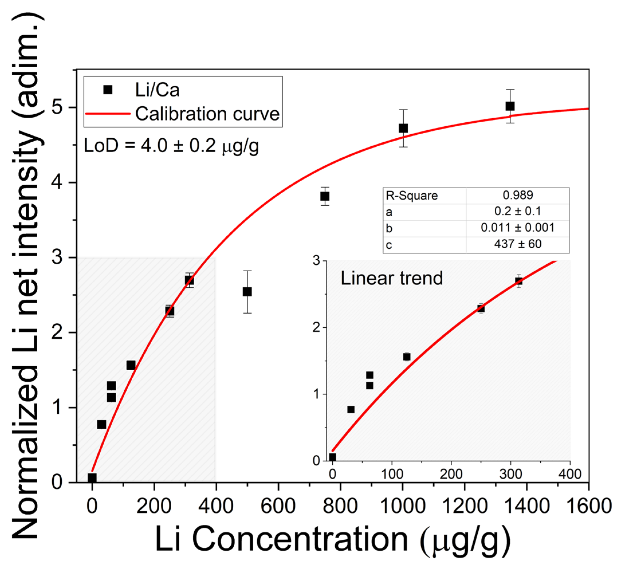
Quantitative analysis of Li in the brine samples was carried out through a calibration curve constructed with the most intense Li I line at 670.77 nm normalized to the neighbor Ca I line at 671.77 nm. The plot of the normalized net intensities of the line 670.77 nm Li I measured from the calibration samples versus the corresponding Li concentrations is shown in Figure 6. The experimental data were fitted to the non-linear function,
where a, b, and c are constant fitting parameters; x represents the concentration; and y is the corresponding normalized intensity [25]. For low concentrations (x << c), Equation (2) is reduced to
which gives the lineal behavior obtained in optically thin plasma conditions. The parameters in Equations (2) and (3) are interpreted as follows: a is the intensity related to zero concentration of the analyte; b is the sensitivity, which is given by the slope of the line in the low concentration region; and c refers to the concentration at which self-absorption of the line becomes noticeable. Moreover, a negative value at the x-axis (i.e., y = 0 and x0 = −a/b) indicated that an initial concentration of Li was detected in the sample matrix as an impurity. The initial Li concentration was 16.4 ± 0.2 µg/g, which was taken into account in the calibration samples. In the calibration curve (Figure 6), it is observed that a linear growth takes place for lower Li concentrations (x ≤ 400 µg/g), where the plasma can be considered as optically thin; then, self-absorption starts to increase at Li concentrations close to xc = 440 µg/g; finally, self-absorption is evident for higher Li concentrations (x ≥ 800 µg/g) as the plasma becomes optically thick.
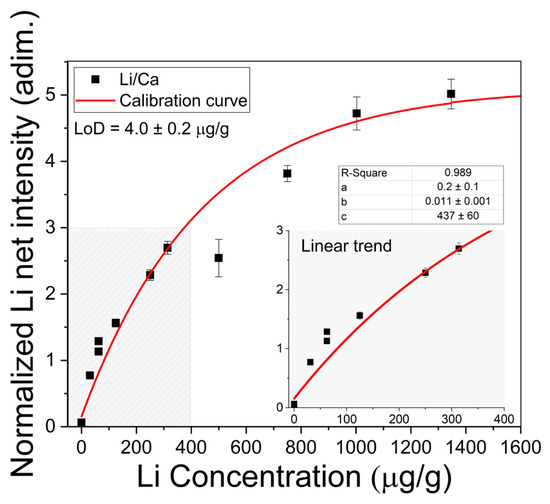
Figure 6.
Calibration curve for Li content with measured Li I 670.77 nm line intensities normalized to Ca I 671.77 nm line intensities. The obtained values for the fitting parameters (a, b, and c) in Equation (2) and the limit of detection (LoD) calculated for brines with Equation (4) are shown. Inset: Linear trend for low Li concentrations.
The detection limit, defined as the concentration that originates a net line intensity equivalent to three times the standard deviation of the background (σB) measured for low concentrations and close to the line profile, was calculated. It was determined by means of the expression [37]
where b is the slope of the linear region of the calibration curve. In our experimental conditions, the calculated limit of detection for Li was LoD = 0.2 ± 0.1 µg/g. The Li concentrations (µg/g) determined in the natural brines are exposed in Table 2. The errors corresponded to the standard deviations of the concentrations obtained for the different measurements in each sample. To assess the accuracy of the LIBS quantitative results, the Li concentrations in the liquid brine solutions were also determined by the conventional AAS technique (Table 2). In Figure 7, it is observed that the results obtained by LIBS and AAS presented similar trends for the different brine samples, denoting the consistency between both techniques. The relatively large difference between LIBS and AAS concentrations observed for sample #11 is attributed to the self-absorption effect due to the higher Li content of this sample. The overall accuracy of the LIBS methodology was evaluated by the averaged quantification error calculated as the normalized standard deviation σN (%),
where qLIBS and qAAS are the Li concentration values calculated with LIBS and AAS techniques, respectively, and n is the number of samples (i.e., n = 11) [22]. A value of σN = 25% was obtained for all the samples analyzed, indicating that the compositional results obtained by LIBS were in a good general agreement with those obtained by AAS (Figure 8).
Table 2.
Li concentrations determined in natural brines by LIBS and AAS techniques.
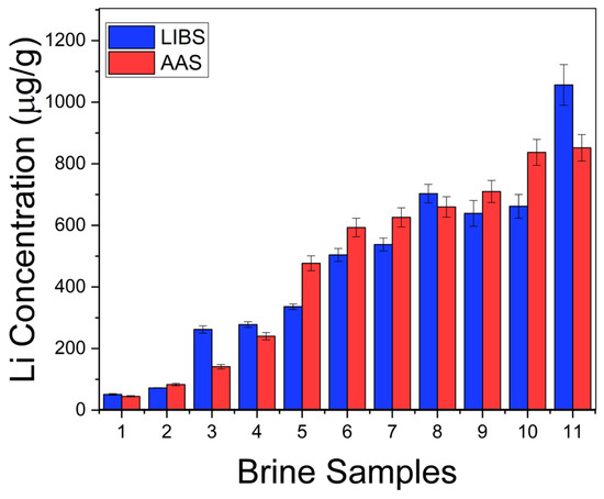
Figure 7.
Li concentration obtained in brines by LIBS and AAS techniques.
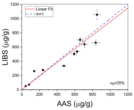
Figure 8.
Crosscheck of LIBS and AAS results. The calculated averaged quantification error (σN%) by Equation (5) is shown. The dotted line corresponds to the ideal situation (m = 1).
4. Conclusions
The LIBS technique was successfully applied for the quantitative analysis of Li-rich continental brines from salars featuring Li concentrations up to 1300 µg/g in a real case study in the Lithium Triangle. The brines were prepared in the form of pellets, which allowed us to overcome the inherent drawbacks of LIBS analysis of liquids. Moreover, under this approach, matrix effects were not observed, which constitutes one of the main challenges in the analysis of environmental samples. The obtained LIBS results were crosschecked with the conventional AAS technique, and a good agreement between both techniques was observed, with an average quantification error of 25. Overall, the analytical methodology and the results presented in this work demonstrated the feasibility of LIBS technology to carry out quantitative analysis of Li in brines. The developed approach is transferable to other salars, and it can also be extended to other valuable elements present in the brines, such as C, Mg, K, Si, and Rb. If necessary, the analytical range can be further extended to account for higher Li concentrations (e.g., Atacama salars [19]) by using for calibration the detected Li I spectral line at 812.26 nm. This non-resonance line has a lower emission intensity, and, thus, it is less sensitive to self-absorption. In a future work, the effects of self-absorption and plasma spatial inhomogeneity on the Li quantification will be investigated in more detail. Moreover, the application of machine-learning methods to analyze big spectral data obtained from the LIBS measurement of a larger number of samples is envisaged. Overall, the information obtained is expected to provide a relevant contribution to and extend the acquired knowledge of the international community of the specific sector.
Author Contributions
Conceptualization, J.M.M., D.M.D.P., C.C.-V., C.S. and A.Y.T.; methodology, J.M.M., D.M.D.P. and C.C.-V.; software, J.M.M. and D.M.D.P.; validation, J.M.M., D.M.D.P., C.C.-V., C.S. and A.Y.T.; formal analysis, J.M.M., D.M.D.P., C.C.-V., C.S. and A.Y.T.; investigation, J.M.M. and D.M.D.P.; resources, J.M.M., D.M.D.P., C.S. and A.Y.T.; data curation, J.M.M. and D.M.D.P.; writing—original draft preparation, J.M.M. and D.M.D.P.; writing—review and editing, J.M.M., D.M.D.P., C.C.-V., C.S. and A.Y.T.; visualization, J.M.M., D.M.D.P. and C.C.-V.; supervision, D.M.D.P. and C.C.-V. All authors have read and agreed to the published version of the manuscript.
Funding
External Postdoctoral grant from CONICET (DDP), grant from the Asociación Universitaria Iberoamericana de Postgrado, AUIP (JMM), and International Association of Sedimentologists (IAS) “Post-Graduate Research Grant” 2nd Session 2018 (CS).
Data Availability Statement
Data analyzed in this manuscript may be shared upon reasonable request.
Acknowledgments
This work was supported by the Consejo Nacional de Investigaciones Científicas y Técnicas (CONICET) of Argentina. JMM and DDP are grateful to J.A. Aguilera, C. Aragón, and M. Zamarbide from the Department of Sciences at UPNA University (Pamplona, Spain) for their assistance during the laboratory analyses. The work was also funded through an External Postdoctoral grant from CONICET (DDP) and a grant from the Asociación Universitaria Iberoamericana de Postgrado, AUIP (JMM). CS acknowledges doctoral fellowship from CONICET and International Association of Sedimentologists (IAS) “Post-Graduate Research Grant” 2nd Session 2018.
Conflicts of Interest
The authors declare no conflicts of interest.
References
- Flexer, V.; Baspineiro, C.F.; Galli, C.I. Lithium recovery from brines: A vital raw material for green energies with a potential environmental impact in its mining and processing. Sci. Total Environ. 2018, 639, 1188–1204. [Google Scholar] [CrossRef] [PubMed]
- Kesler, S.E.; Gruber, P.W.; Medina, P.A.; Keoleian, G.A.; Everson, M.P.; Wallington, T.J. Global lithium resources: Relative importance of pegmatites, brine and other deposits. Ore Geol. Rev. 2012, 48, 44–69. [Google Scholar] [CrossRef]
- Steinmetz, R.L.L.; Salvi, S. Brine grades in Andean salars: When basin size matters—A review of the Lithium Triangle. Earth-Sci. Rev. 2021, 217, 103615. [Google Scholar] [CrossRef]
- BP, Statistical Review of World Energy 2022, 71st ed., BP p.l.c. 2022. Available online: https://www.bp.com/statisticalreview (accessed on 3 September 2024).
- Steinmetz, R.L.; Salvi, S.; García, M.G.; Arnold, Y.J.P.; Béziat, D. Northern Puna Plateau-scale survey of Li brine-type deposits in the Andes of NW Argentina. J. Geochem. Explor. 2018, 190, 26–38. [Google Scholar] [CrossRef]
- Bustos-Gallardo, B.; Bridge, G.; Prieto, M. Harvesting Lithium: Water, brine and the industrial dynamics of production in the Salar de Atacama. Geoforum 2021, 119, 177–189. [Google Scholar] [CrossRef]
- Miziolek, A.W.; Palleschi, V.; Schechter, I. Laser-Induced Breakdown Spectroscopy (LIBS) Fundamentals and Applications; Cambridge University Press: New York, NY, USA, 2006. [Google Scholar] [CrossRef]
- Hahn, D.W.; Omenetto, N. Laser-induced breakdown spectroscopy (LIBS), part I: Review of basic diagnostics and plasma–particle interactions. Appl. Spectrosc. 2010, 64, 335A–366A. [Google Scholar] [CrossRef]
- Winefordner, J.D.; Gornushkin, I.B.; Correll, T.; Gibb, E.; Smith, B.W.; Omenetto, N. Comparing several atomic spectrometric methods to the super stars: Special emphasis on laser-induced breakdown spectrometry, LIBS, a future super star. J. Anal. At. Spectrom. 2004, 19, 1061–1083. [Google Scholar] [CrossRef]
- Hahn, D.W.; Omenetto, N. Laser-induced breakdown spectroscopy (LIBS), part II: Review of instrumental and methodological approaches. Appl. Spectrosc. 2012, 66, 347–419. [Google Scholar] [CrossRef]
- Tognoni, E.; Cristoforetti, G.; Legnaioli, S.; Palleschi, V. Calibration-Free Laser-Induced Breakdown Spectroscopy: State of the art. Spectrochim. Acta Part B 2010, 65, 1–14. [Google Scholar] [CrossRef]
- Harmon, R.S.; Russo, R.E.; Hark, R.R. Applications of laser-induced breakdown spectroscopy for geochemical and environmental analysis: A comprehensive review. Spectrochim. Acta Part B 2013, 87, 11–26. [Google Scholar] [CrossRef]
- Ytsma, C.R.; Dyar, M.D. Accuracies of lithium, boron, carbon, and sulfur quantification in geological samples with laser-induced breakdown spectroscopy. Spectrochim. Acta Part B 2019, 162, 105715. [Google Scholar] [CrossRef]
- Ferreira, M.F.S.; Capela, D.; Silva, N.A.; Gonçalves, F.; Lima, A.; Guimaraes, D.; Jorge, P.A.S. Comprehensive comparison of linear and non-linear methodologies for lithium quantification in geological samples using LIBS. Spectrochim. Acta Part B 2022, 195, 106504. [Google Scholar] [CrossRef]
- St-Onge, L.; Kwong, E.; Sabsabi, M.; Vadas, E.B. Rapid analysis of liquid formulations containing sodium chloride using laser–induced breakdown spectroscopy. J. Pharm. Biomed. Anal. 2004, 36, 277–284. [Google Scholar] [CrossRef]
- Bordel, N.; Fernández, L.J.; Méndez, C.; González, C.; Pisonero, J. Halides formation dynamics in nanosecond and femtosecond laser-induced breakdown spectroscopy. Plasma Phys. Control. Fusion. 2022, 64, 054010. [Google Scholar] [CrossRef]
- Aragón, C.; Aguilera, J.A.; Manrique, J. Measurement of Stark broadening parameters of FeII and NiII spectral lines by laser induced breakdown spectroscopy using fused glass samples. J. Quant. Spectrosc. Radiat. Transf. 2014, 134, 39–45. [Google Scholar] [CrossRef]
- Lal, B.; Zheng, H.; Yueh, F.Y.; Singh, J.P. Parametric study of pellets for elemental analysis with laser-induced breakdown spectroscopy. Appl. Opt. 2004, 43, 2792–2797. [Google Scholar] [CrossRef]
- Erbetta, N.; Puebla, G.; Day, D.; Jennings, M.; Loureiro, A.; Green, C.; Gallardo, L.; Quiroz, W. Direct determination of lithium in brine samples using handheld LIBS without sample treatment: Sample introduction by venturi system. Anal. Methods 2024, 16, 7311–7318. [Google Scholar] [CrossRef]
- Xing, P.; Dong, J.; Yu, P.; Zheng, H.; Xing, L.; Hu, S.; Zhu, Z. Quantitative analysis of lithium in brine by LIBS based on convolutional neural network. Anal. Chim. Acta 2021, 1178, 338799. [Google Scholar] [CrossRef]
- Díaz Pace, D.M.; D’Angelo, C.A.; Bertuccelli, D.; Bertuccelli, G. Analysis of heavy metals in liquids using LIBS by liquid-to-solid matrix conversion. Spectrochim. Acta Part B 2006, 61, 929–933. [Google Scholar] [CrossRef]
- Terán, E.J.; Montes, M.L.; Rodríguez, C.; Martino, L.; Quiroga, M.; Landa, R.; Sánchez, R.M.T.; Díaz Pace, D.M. Assessment of sorption capability of montmorillonite clay for lead removal from water using laser–induced breakdown spectroscopy and atomic absorption spectroscopy. Microchem. J. 2019, 144, 159–165. [Google Scholar] [CrossRef]
- Garcimuño, M.; Díaz Pace, D.M.; Bertuccelli, G. Laser-induced breakdown spectroscopy for quantitative analysis of copper in algae. Opt. Laser Technol. 2013, 47, 26–30. [Google Scholar] [CrossRef]
- Díaz Pace, D.M.; D’Angelo, C.A.; Bertuccelli, G. Study of self-absorption of emission magnesium lines in laser-induced plasmas on calcium hydroxide matrix. IEEE Trans. Plasma Sci. 2012, 40, 898–908. [Google Scholar] [CrossRef]
- Díaz Pace, D.M.; D’Angelo, C.A.; Bertuccelli, G. Calculation of Optical Thicknesses of Magnesium Emission Spectral Lines for Diagnostics of Laser-Induced Plasmas. Appl. Spectrosc. 2011, 65, 1202–1212. [Google Scholar] [CrossRef] [PubMed]
- American Public Health Association. Standard Methods for the Examination of Water and Wastewater; American Public Health Association: Washington, DC, USA, 2023; pp. 16–17. [Google Scholar]
- National Institute of Standards and Technology (NIST). Atomic Spectra Database. 2022. Available online: https://www.nist.gov/pml/atomic-spectra-database (accessed on 7 July 2024).
- Griem, H.R. Plasma Spectroscopy; McGraw-Hill: New York, NY, USA, 1964. [Google Scholar]
- McWhirter, R.W.P.; Huddlestone, R.H.; Leonard, S.L. (Eds.) Plasma Diagnostic Techniques; Academic Press: New York, NY, USA, 1965; pp. 201–264, Chapter 5. [Google Scholar]
- Gigosos, M.A.; Cardenoso, V. New plasma diagnosis tables of hydrogen Stark broadening including ion dynamics. J. Phys. B At. Mol. Opt. Phys. 1996, 29, 4795–4838. [Google Scholar] [CrossRef]
- Aragón, C.; Bengoechea, J.; Aguilera, J.A. Influence of the optical depth on spectral line emission from laser-induced plasmas. Spectrochim. Acta Part B 2001, 56, 619–628. [Google Scholar] [CrossRef]
- Díaz Pace, D.M.; Miguel, R.E.; Di Rocco, H.O.; García, F.A.; Pardini, L.; Legnaioli, S.; Lorenzetti, G.; Palleschi, V. Quantitative analysis of metals in waste foundry sands by calibration-free laser induced breakdown spectroscopy. Spectrochim. Acta Part B 2017, 131, 58–65. [Google Scholar] [CrossRef]
- El Sherbini, A.M.; Hegazy, H.; El Sherbini, T.M. Measurement of electron density utilizing the H Alpha-line from laser produced plasma in air. Spectrochim. Acta Part B 2006, 61, 532–539. [Google Scholar] [CrossRef]
- Parigger, C.G.; Surmick, D.M.; Gautam, G.; El Sherbini, A.M. Hydrogen alpha laser ablation plasma diagnostics. Opt. Lett. 2015, 40, 3436–3439. [Google Scholar] [CrossRef]
- Konjević, N.; Ivković, M.; Jovićević, S. Spectroscopic diagnostics of laser-induced plasmas. Spectrochim. Acta Part B 2010, 65, 593–602. [Google Scholar] [CrossRef]
- Aguilera, J.A.; Aragón, C. Characterization of a laser-induced plasma by spatially resolved spectroscopy of neutral atom and ion emissions. Spectrochim. Acta Part B 2004, 59, 1861–1876. [Google Scholar] [CrossRef]
- Sabsabi, M.; Cielo, P. Quantitative analysis of aluminum alloys by laser induced breakdown spectroscopy and plasma characterization. Appl. Spectrosc. 1995, 49, 499–507. [Google Scholar] [CrossRef]


Disclaimer/Publisher’s Note: The statements, opinions and data contained in all publications are solely those of the individual author(s) and contributor(s) and not of MDPI and/or the editor(s). MDPI and/or the editor(s) disclaim responsibility for any injury to people or property resulting from any ideas, methods, instructions or products referred to in the content. |
© 2025 by the authors. Licensee MDPI, Basel, Switzerland. This article is an open access article distributed under the terms and conditions of the Creative Commons Attribution (CC BY) license (https://creativecommons.org/licenses/by/4.0/).