An Explicit Numerical Scheme for Milne’s Phase–Amplitude Equations

Abstract

We present an explicit numerical method to solve Milne’s phase–amplitude equations. Existing methods directly solve Milne’s nonlinear equation for amplitude. For that reason, they exhibit high sensitivity to errors and are prone to instability through the growth of a spurious, rapidly varying component of the amplitude. This makes the systematic use of these methods difficult. On the contrary, the present method is based on solving a linear third-order equation which is equivalent to the nonlinear amplitude equation. This linear equation was derived by Kiyokawa, who used it to obtain analytical results on Coulomb wavefunctions. The present method uses this linear equation for numerical computation, thus resolving the problem of the growth of a rapidly varying component.

1. Introduction

Accurate modeling of atomic processes in plasmas such as collisional excitation, photoionization, and Bremsstrahlung requires a precise computation of radial wavefunctions for continuum electron orbitals. In dense plasmas, one should in principle account self-consistently for continuum electrons in the calculation of the atomic structure (see, e.g., [1,2,3] for discussions on this subject). A rigorous approach requires sampling these oscillatory radial wavefunctions in both radius and momentum spaces (e.g., [4,5,6,7]), with the minimal requirement for sampling being governed by the Nyquist–Shannon theorem [8]. The latter constraint leads to a significant computational burden—demanding both substantial memory and substantial floating-point operations—which often hinders the feasibility of self-consistent, quantum-mechanical modeling of plasmas.

Alternative approaches to representing the one-electron basis can offer more efficient numerical solutions. Recently, Starrett et al. [9] proposed an average-atom algorithm based on Siegert states, building on the method of [10]. However, retaining a more conventional one-electron basis, Milne’s phase–amplitude representation [11] also provides an alternative pathway to efficiently represent the continuum. Being based on slowly varying, non-periodic amplitude and phase functions, it circumvents the stringent sampling requirements of the Nyquist–Shannon theorem and has long been recognized for its numerical advantages. It has been successfully applied to calculations of Bessel functions [12] and atomic physics problems [5,13,14]. Various solution methods have been proposed, including direct iterative schemes [15,16], spectral methods using Chebyshev expansions [17], and explicit predictor–corrector methods [13] implemented in codes like SCROLL [18] and HULLAC [19], as well as adaptive mesh refinement Rosenbrock methods [14] used in PURGATORIO [5].

Despite these advances, existing methods usually do not allow for simple and systematic use on a pre-defined grid, with a simple relationship between grid coarseness and precision. In particular, they show a rather high sensitivity to numerical errors. In this article, we first review the fundamentals of Milne’s phase–amplitude representation. We then discuss the limitations of some previously published methods [5,13,14]. Finally, we present a fully explicit, fixed-grid method based on solving a linear third-order equation, initially derived by Kiyokawa [20], which is equivalent to the nonlinear amplitude equation. This numerical method addresses the limitations mentioned, and we demonstrate its application on the illustrative example of phase-shift calculations.

2. Phase–Amplitude Representations

In the following, we will limit the discussion to the description of continuum radial wavefunctions $R\left(r\right)$, solutions of the radial Schrödinger equation:

$$\begin{array}{cc}\hfill & \hfill R^{″}\left(r\right)+{\omega }_{k,\ell }\left(r\right)R\left(r\right)=0\hfill \end{array}$$

(1)

$$\begin{array}{cc}\hfill & \hfill {\omega }_{k,\ell }\left(r\right)=k^2-2v\left(r\right)-{\displaystyle \frac{\ell (\ell +1)}{r^2}}\hfill \end{array}$$

(2)

where $k^2>0$ and ${lim}_{r\to \infty }v\left(r\right)=0$. Most phase–amplitude (PA) representations may also be extended to bound states, considering an imaginary k. Moreover, PA representations can also be used in the framework of the Dirac radial equation set without any difficulty (see, for instance, [21], Section 2.3).

Phase–amplitude representation refers to a whole category, rather to a particular representation. Such representations consist of recasting the oscillatory wavefunction R, regular at zero, as follows:

$$\begin{array}{c}\hfill R\left(r\right)=A\left(r\right)·S\left(\varphi \left(r\right)\right)\end{array}$$

(3)

where S is a given oscillatory function regular at zero. $A\left(r\right)$ is called the amplitude function, and $\varphi \left(r\right)$ is the phase function.

Generalized PA representation may resort to any oscillatory function S corresponding to the regular solution of the Schrödinger equation for some reference system. The generalized Wentzel–Kramers–Brillouin (WKB) approach [22,23,24,25] may be considered from this standpoint.

In the present article, we focus on Milne’s PA representation, which uses a sine function for S.

$$\begin{array}{c}\hfill R\left(r\right)=A\left(r\right)·sin\left(\varphi \left(r\right)\right)\end{array}$$

(4)

The choice of a particular function S is not sufficient to completely determine the representation. In particular, the choice of the sine function for S is used in both Calogero’s and Milne’s PA representations.

Just to highlight their differences, let us briefly recall the basics of Calogero’s PA representation [26]. To obtain this PA representation, one requires, in addition to Equation (4), the following:

$$\begin{array}{c}\hfill R^{\prime }\left(r\right)=A\left(r\right)·cos\left(\varphi \left(r\right)\right)\end{array}$$

(5)

Therefore,

$$\begin{array}{cc}\hfill & \hfill A\left(r\right)=\sqrt{R{\left(r\right)}^2+R^{\prime }{\left(r\right)}^2}\hfill \end{array}$$

(6)

$$\begin{array}{cc}\hfill & \hfill tan\left(\varphi \left(r\right)\right)={\displaystyle \frac{R\left(r\right)}{R^{\prime }\left(r\right)}}\hfill \end{array}$$

(7)

Since $R\left(r\right)$ is regular at zero, Calogero’s amplitude function is regular at zero. Re-writing Equation (1) and using Equations (4) and (5) yields Calogero’s equations for phase and amplitude (see [26], Equations (6.16) and (4.7)):

$$\begin{array}{c}\hfill {\varphi }^{\prime }\left(r\right)=k+{\displaystyle \frac{1}{k}}\left(k^2-{\omega }_{k,\ell }\left(r\right)\right){sin}^2\left(\varphi \left(r\right)\right)\end{array}$$

(8)

$$\begin{array}{c}\hfill A^{\prime }\left(r\right)=A\left(r\right)\left(k^2-{\omega }_{k,\ell }\left(r\right)\right){\displaystyle \frac{sin\left(2\varphi \left(r\right)\right)}{2k}}\end{array}$$

(9)

From these equations, it appears clearly that the amplitude and phase functions of Calogero’s PA representation exhibit rapid variations, i.e., on the scale of r∼1/(2k). This representation was used to derive many useful analytical results in scattering theory [27], such as an analytic approximation to phase shifts in screened potentials [28]. Calogero’s PA representation was also used in order to build efficient numerical methods for searching the eigenvalues of bound states in an attractive potential [29,30]. However, when applied to continuum orbitals, this representation requires the same typical sampling of $A\left(r\right)$ and $\varphi \left(r\right)$ as the radial wavefunction itself.

Milne’s PA representation is most often derived by inserting Equation (4) into Equation (1), yielding

$$\begin{array}{c}\hfill \left[2A^{\prime }\left(r\right){\varphi }^{\prime }\left(r\right)+A\left(r\right){\varphi }^{″}\left(r\right)\right]cos\left(\varphi \left(r\right)\right)+\left[A^{″}\left(r\right)-A\left(r\right){\left({\varphi }^{\prime }\left(r\right)\right)}^2+{\omega }_{k,\ell }\left(r\right)A\left(r\right)\right]sin\left(\varphi \left(r\right)\right)=0\end{array}$$

(10)

One then requires the factors in front of the sine and cosine of the phase to be zero independently. This leads to Milne’s equations for the phase and amplitude, respectively,

$$\begin{array}{cc}\hfill & \hfill {\varphi }^{\prime }\left(r\right)={\displaystyle \frac{\theta }{A{\left(r\right)}^2}}\hfill \end{array}$$

(11)

$$\begin{array}{cc}\hfill & \hfill A^{″}\left(r\right)+{\omega }_{k,\ell }\left(r\right)A\left(r\right)-{\displaystyle \frac{{\theta }^2}{A{\left(r\right)}^3}}=0\hfill \end{array}$$

(12)

with $\theta$ appearing as an arbitrary integration constant.

A somewhat more explicit definition of Milne’s phase and amplitude may be stated as follows. Let us consider $R\left(r\right)$, $Q\left(r\right)$ two linearly independent solutions of Equation (1), with $R\left(r\right)$ being regular at $r=0$, and define $A\left(r\right)$ and $\varphi \left(r\right)$ as follows:

$$\begin{array}{c}\hfill R\left(r\right)=A\left(r\right)·sin\left(\varphi \left(r\right)\right)\end{array}$$

(13)

$$\begin{array}{c}\hfill Q\left(r\right)=A\left(r\right)·cos\left(\varphi \left(r\right)\right)\end{array}$$

(14)

One has

$$\begin{array}{cc}\hfill & \hfill A\left(r\right)=\sqrt{R{\left(r\right)}^2+Q{\left(r\right)}^2}\hfill \end{array}$$

(15)

$$\begin{array}{cc}\hfill & \hfill tan\left(\varphi \left(r\right)\right)={\displaystyle \frac{R\left(r\right)}{Q\left(r\right)}}\hfill \end{array}$$

(16)

Differentiating Equation (16), one obtains

$$\begin{array}{cc}\hfill \left(1+{tan}^2\left(\varphi \left(r\right)\right)\right){\varphi }^{\prime }\left(r\right)& \hfill ={\displaystyle \frac{Q\left(r\right)R^{\prime }\left(r\right)-R\left(r\right)Q^{\prime }\left(r\right)}{Q{\left(r\right)}^2}}\hfill \end{array}$$

(17)

$$\begin{array}{cc}\hfill {\varphi }^{\prime }\left(r\right)& \hfill ={\displaystyle \frac{\mathcal{W}\left\{Q\right(r),R(r\left)\right\}}{A{\left(r\right)}^2}}\hfill \end{array}$$

(18)

where $\mathcal{W}$ denotes the Wronskian. Differentiating Equation (15) two times, one obtains

$$\begin{array}{cc}\hfill A^{″}\left(r\right)=& \hfill {\displaystyle \frac{-1}{A{\left(r\right)}^2}}{A}^{\prime }\left(r\right)\left[R\left(r\right)R^{\prime }\left(r\right)+Q\left(r\right)Q^{\prime }\left(r\right)\right]\hfill \\ \hfill & \hfill +{\displaystyle \frac{1}{A\left(r\right)}}\left[R\left(r\right)R^{″}\left(r\right)+R^{\prime }{\left(r\right)}^2+Q\left(r\right)Q^{″}\left(r\right)+Q^{\prime }{\left(r\right)}^2\right]\hfill \end{array}$$

(19)

Using Equation (1) for $R\left(r\right)$ and $Q\left(r\right)$, and the definition of Equation (15), one obtains

$$\begin{array}{cc}\hfill A^{″}\left(r\right)=& \hfill -{\omega }_{k,\ell }\left(r\right)A\left(r\right)-{\displaystyle \frac{1}{A\left(r\right)}}\left[A^{\prime }{\left(r\right)}^2-R^{\prime }{\left(r\right)}^2-Q^{\prime }{\left(r\right)}^2\right]\hfill \end{array}$$

(20)

$$\begin{array}{cc}\hfill =& \hfill -{\omega }_{k,\ell }\left(r\right)A\left(r\right)+{\displaystyle \frac{\mathcal{W}{\{Q\left(r\right),R\left(r\right)\}}^2}{A{\left(r\right)}^3}}\hfill \end{array}$$

(21)

Defining $\theta =\mathcal{W}\left\{Q\right(r),R(r\left)\right\}$, Equations (18) and (21) become Equations (11) and (12), respectively. This derivation has the advantage of showing explicitly how $\theta$ is related to the normalizations of the R and Q functions.

Two particular cases are those of free particles ($v\left(r\right)=0$) and particles in a Coulomb potential ($v\left(r\right)=-Z/r$). For these, one has the following analytical solutions:

$$\begin{array}{c}\hfill R\left(r\right)=\left\{\begin{array}{cc}\hfill kr{j}_{\ell }\left(kr\right)\hfill & \hfill \left(v\left(r\right)=0\right)\hfill \\ \hfill F_{\ell }(\eta =-Z/k,kr)\hfill & \hfill \left(v\left(r\right)=-Z/r\right)\hfill \end{array}\right.\end{array}$$

(22)

$$\begin{array}{c}\hfill Q\left(r\right)=\left\{\begin{array}{cc}\hfill -kr{y}_{\ell }\left(kr\right)\hfill & \hfill \left(v\left(r\right)=0\right)\hfill \\ \hfill G_{\ell }(\eta =-Z/k,kr)\hfill & \hfill \left(v\left(r\right)=-Z/r\right)\hfill \end{array}\right.\end{array}$$

(23)

where $j_{\ell }$ and $y_{\ell }$ are the regular and irregular spherical Bessel functions, respectively, and $F_{\ell }$ and $G_{\ell }$ are the regular and irregular Coulomb wavefunctions. We use the conventions of [31]. The latter analytical solutions can be used together with Equation (15) for the evaluation of the boundary condition for fully screened and Coulomb-tail atomic potentials, respectively.

Equation (12) is a second-order nonlinear differential equation. Its solutions are nontrivial. However, in the asymptotic limit $r\to \infty$, Equation (12) simply becomes

$$\begin{array}{cc}\hfill & \hfill A^{″}\left(r\right)+k^{2}A\left(r\right)-{\displaystyle \frac{{\theta }^2}{A{\left(r\right)}^3}}=0\hfill \end{array}$$

(24)

One readily see that a constant $A\left(r\right)$ can be solution of this equation, with its value being

$$\begin{array}{cc}\hfill & \hfill A_{\mathrm{slow}}={\left({\displaystyle \frac{\theta }{k}}\right)}^{1/2}\hfill \end{array}$$

(25)

This directly yields ${\varphi }_{\mathrm{slow}}\left(r\right)\sim kr$ using Equation (11).

This asymptotic limit may also be recovered from the usual WKB approximation, which just consists of neglecting the second derivative $A^{″}\left(r\right)$ in Equation (12), yielding:

$$\begin{array}{cc}\hfill & \hfill A_{\mathrm{WKB}}\left(r\right)={\displaystyle \frac{{\theta }^{1/2}}{{\omega }_{k,\ell }{\left(r\right)}^{1/4}}}\underset{r\to \infty }{\to }{A}_{\mathrm{slow}}\hfill \end{array}$$

(26)

$$\begin{array}{cc}\hfill & \hfill {\varphi }_{\mathrm{WKB}}^{\prime }\left(r\right)={\omega }_{k,\ell }{\left(r\right)}^{1/2}\underset{r\to \infty }{\to }k\hfill \end{array}$$

(27)

Let us stress that the parameter $\theta$ is related through Equation (25) to the asymptotic value of the amplitude function, which determines the normalization of $R\left(r\right)$. Therefore, $\theta$ has to be consistent with the boundary condition applied when solving Equation (12) for the amplitude. Having a parameter in the equation which has to be consistent with the boundary condition is typical for a nonlinear equation. On the contrary, linear equations allow the boundary condition to be set with an arbitrary multiplicative constant.

The solution of Equation (12) fulfilling the condition ${lim}_{r\to \infty }{A}^{″}\left(r\right)=0$ corresponds to a slowly varying amplitude function, asymptotically tending to the value $A_{\mathrm{slow}}$. This is the amplitude function we are interested in, as it allows us to circumvent the Nyquist–Shannon sampling limit related to the oscillatory wavefunction $R\left(r\right)$.

However, Equation (12) may have other solutions than the slowly varying one. Returning to its asymptotic limit Equation (24), let us try to find another solution by considering a first-order perturbation $A_{\mathrm{slow}}+\delta A\left(r\right)$ around the constant solution of Equation (25). The equation for the perturbation is

$$\begin{array}{cc}\hfill & \hfill \delta A^{″}\left(r\right)+k^2\delta A\left(r\right)+3{\displaystyle \frac{{\theta }^2}{A_{\mathrm{slow}}^4}}\delta A\left(r\right)=0\hfill \end{array}$$

(28)

$$\begin{array}{cc}\hfill & \hfill \delta A^{″}\left(r\right)=-4k^2\delta A\left(r\right)\hfill \end{array}$$

(29)

From this equation, we get $\delta A\left(r\right)\sim e^{2ikr}$, showing that other solutions exist and that they exhibit rapid variation, i.e., over the $1/\left(2k\right)$ scale.

Equation (12) is thus a stiff differential equation in the sense that it has multiple solutions varying over very different scales. However, for the purpose of a sampling reduction, we are only interested in the slowly varying one. Moreover, being nonlinear, this equation can allow coupling among its various solutions, which may constitute a problem, as we will see in the next section.

For the sake of illustrating the slowly varying amplitude function of Milne’s PA representation, in Figure 1, we present the radial wavefunctions $R\left(r\right)$ and the corresponding amplitude functions $A\left(r\right)$, for $k=1a_0^{-1}$, $\ell =2$, in the case of a zero potential (a), of a screened Coulomb potential (b), and of a pure Coulomb potential (c). The slowly varying amplitude functions correspond to the envelopes of the related wavefunctions.

Of course, the amplitude function can be obtained from a numerical solution of Equation (1), by finding the two linearly independent solutions R and Q and then combining them as in Equation (15). However, such a method would require sampling oscillatory functions, thus defeating the purpose of using the PA representation.

Thus, a number of authors have studied numerical methods for solving Equation (12) directly. Seaton and Peach, as well as Trafton, proposed iterative schemes, starting from an initial guess of the amplitude [15,16]. Bar Shalom et al. [13] proposed to use a predictor–corrector scheme due to Hamming (see [32] Sec. 24.3) when it is stable, and they proposed a modified predictor–corrector scheme for the region in which Hamming’s method is unstable. Wilson et al. [5,14] proposed to use a Kaps–Rentrop method [33,34]. Rawitscher [17] proposed a spectral iterative method based on a Chebyshev expansion.

In atomic physics applications, description of the continuum usually requires the calculation of a large number of wavefunctions in order to sample the momentum space. There is thus a special interest in fast, fully explicit numerical methods, such as that proposed in [13]. Before coming to the method that we propose, let us first present our motivation for the present work by discussing the limitation of some existing methods.

3. Limitations of Some Existing Methods

Bar Shalom et al. [13] propose an explicit method to numerically solve Equation (12) on a fixed grid of exponentially spaced points. The method in fact resorts to three distinct numerical schemes. We briefly recall its general principle below, as it guided many aspects of our method’s development.

In the innermost region, a standard Numerov scheme is used to solve Equation (1) for $R\left(r\right)$, up to a matching point $r_{\mathrm{match}}$, chosen close to the turning point $r_{\mathrm{turn}}$, such that ${\omega }_{k,\ell }\left(r_{\mathrm{turn}}\right)=0$.

Beyond the matching point, Bar Shalom et al. [13] use a predictor–corrector method due to Hamming (see [32] Sec. 24.3) in order to solve Equation (12) for $A\left(r\right)$. Let us call this scheme Hamming’s predictor–corrector (HPC). However, they find that, as soon as $h^2{\omega }_{k,\ell }\left(r\right)/3$ is greater than one, then the corrector step amplifies the prediction error. Far from the origin, the slowly varying amplitude solution tends to a constant. Thus, $A^{″}\left(r\right)$ takes small values which are obtained through Equation (12) as differences between two values that are comparatively large. This leads to large numerical errors, and this issue is common to all approaches that make use of Equation (12) to obtain $A^{″}\left(r\right)$ from $A\left(r\right)$.

As a solution to this problem, Bar Shalom et al. [13] propose a modified predictor–corrector scheme for the outermost region. Its basic principle is to use the fact that $A\left(r\right)$ varies slowly to build a predictor for $A^{″}\left(r\right)$ and then use Equation (12) as a corrector, deducing a new value of $A\left(r\right)$ from $A^{″}\left(r\right)$. This is carried out performing one step of a Newton method. Using the amplitude equation in this other way, the error amplification factor is inverted, leading to a stable scheme. Let us call this scheme Bar Shalom’s modified predictor–corrector (BSMPC).

In addition to the BSMPC scheme, the authors suggest to further improve the solution in the outermost region by re-evaluating $A^{″}\left(r\right)$ from a high-order finite-difference scheme (five-point scheme) and correcting again using Equation (12). Adding such a step makes the method become partly an iterative method, and we did not find such an improvement useful in the present study.

The switching radius $r_{\mathrm{switch}}$ from the HPC to BSMPC scheme is located where $h^2{\omega }_{k,\ell }\left(r\right)/3\approx 1$, and these two schemes are actually employed in order to propagate the solution inwards, starting from the outer boundary condition at $r_{\max }$. Finally, solutions for $R\left(r\right)$ and $A\left(r\right)$ are matched at the radius $r_{\mathrm{match}}$, allowing one to normalize $R\left(r\right)$ and determine the phase at the matching point. A summary of this method is given in

Table 1. Summary of the numerical method proposed in [13].

Innermost Region	Intermediate Region	Outermost Region
$[{\mathit{r}}_{\min },{\mathit{r}}_{\mathrm{match}}]$	$[{\mathit{r}}_{\mathrm{match}},{\mathit{r}}_{\mathrm{switch}}]$	$[{\mathit{r}}_{\mathrm{switch}},{\mathit{r}}_{\max }]$
$h^2{\omega }_{k,\ell }\left(r\right)/3<1$	$h^2{\omega }_{k,\ell }\left(r\right)/3<1$	$h^2{\omega }_{k,\ell }\left(r\right)/3>1$
Numerov scheme for $R\left(r\right)$	Hamming’s predictor–corrector	Bar Shalom’s modified predictor–corrector
Outwards	Inwards	Inwards

.

We found that the numerical method proposed in [13] performs very well on coarse grids. As described in their article, one really needs to apply both HPC and BSMPC schemes, paying attention to the switching radius $r_{\mathrm{switch}}$. We verified that error amplification actually occurs when using any of the numerical schemes on the wrong side of $r_{\mathrm{switch}}$, and found that the overall method is very sensitive to such error amplification.

In his book, Hamming derives a predictor–corrector numerical scheme of order 6. He also describes corrections to the predictor and corrector (see [32], end of Sec. 24.3), which are presented as optional, and makes the scheme of order 8. We found that in the present case, these corrections are required for the global stability of the numerical method, and we assume that Bar Shalom and his coauthors did use these corrections.

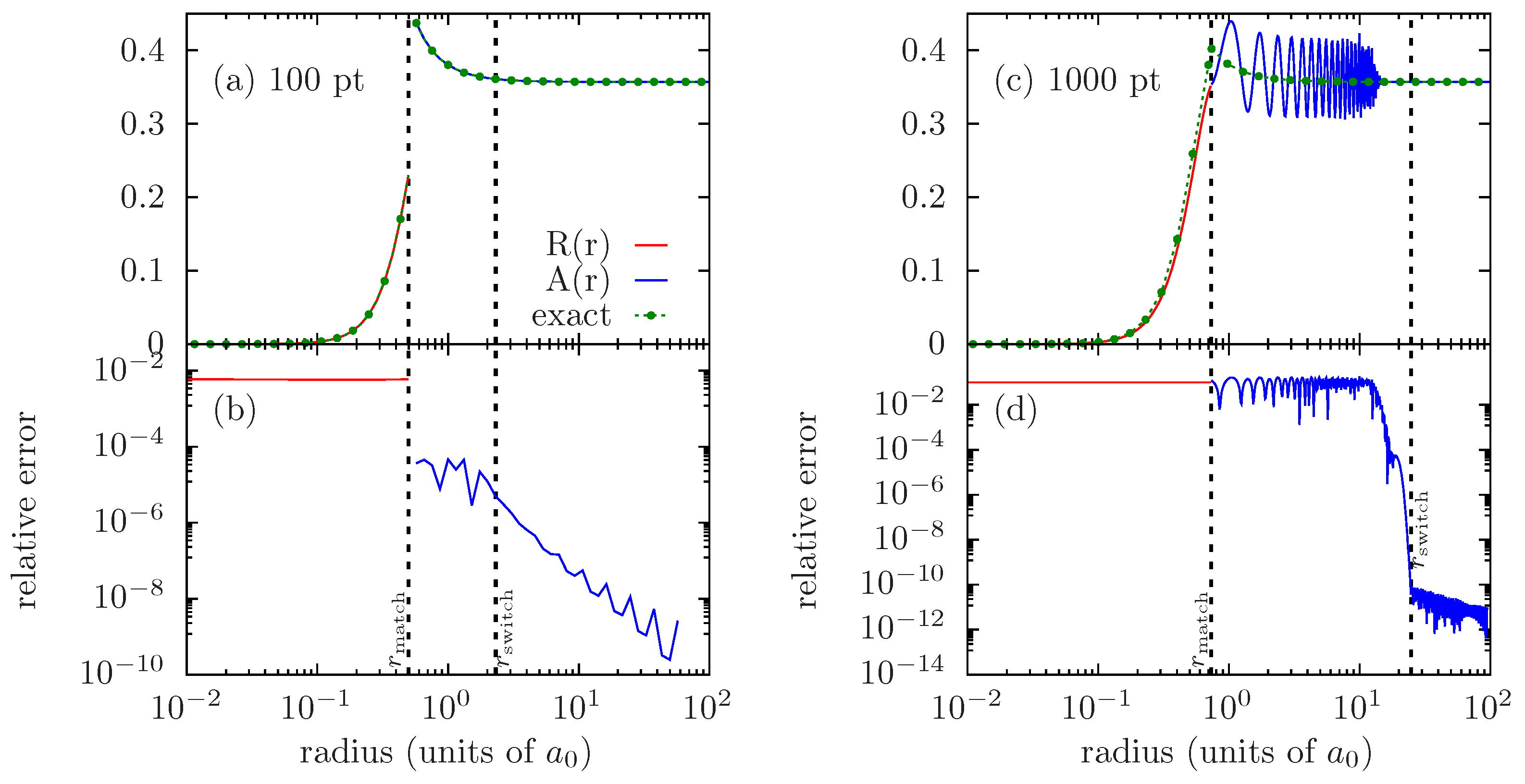
In principle, if one wants to increase the precision of the solution, refining the grid should be the way to proceed. It turns out that beyond a certain level of refinement, a numerical instability occurs, ruining the numerical solution. This issue is illustrated in Figure 2, which displays the results obtained in a case of zero potential (amplitude of spherical Bessel functions) when increasing the number of grid points from 100 to 1000.

The triggering of an instability when considering finer grids constitutes a serious limitation to the systematic use of this numerical scheme, as it impairs the control of the numerical precision.

In Figure 2d, one may clearly identify a region of strong increase in errors. This region seems to always lie in the intermediate region, where the HPC scheme is used. By applying the predictor–corrector scheme step by step on a test case for which the solution is known exactly, one may precisely analyze the source of errors. By restarting at each step from the “exact” amplitude, one can see that the error growth is driven by the predictor; on the other hand, the corrector systematically improves the solution as expected.

An explanation for this large increase in error may be the nonlinear character of Equation (12). In principle, it allows for the coupling among various solutions and enables the growth of a spurious, rapidly varying component in the solution, starting from an initial seed.

In principle, we select the desired, slowly varying solution through the boundary condition. However, any error, either the truncation error on the boundary condition or the accumulation of numerical errors when propagating the solution, may be seen as a mix between the desired solution and the spurious ones, seeding the growth of the rapidly varying component.

A numerical limitation to the growth of a rapidly varying component is the sampling. A coarse grid acts as a low-pass filter and may temper the growth of a rapidly varying component. It turns out that the criterion for switching from the HPC to BSMPC is close to the Nyquist–Shannon sampling criterion for the rapidly varying solution. This probably explains why the region where the spurious component builds up is located inside the intermediate region, near the switching radius.

Regardless of the method used, any attempt to directly solve the nonlinear Equation (12) is likely to yield a result which is strongly sensitive to errors and prone to the growth of a rapidly varying component in the amplitude. This notably explains the crucial need for a high-order scheme in the method of [13] and why the corrections which allow one to reach order 8 matter so much.

In [5,14], the authors used a Rosenbrock method proposed by Kaps and Rentrop [33], which is frequently used for stiff equations [34]. Typical numerical methods for stiff equations are usually based on adaptive grid refinement, aiming at correctly sampling all solutions, with all their various scales of variation.

Certainly, Equation (12) is stiff, but our purpose is only to calculate its slowly varying solution, and not to achieve a correct sampling of all of its solutions. In this view, it is likely that such methods are of limited help for the present problem. However, using a very stringent precision target, adaptive grid refinement may also limit the accumulation of errors, therefore limiting the seed for a spurious component. One should, however, keep in mind that, in many cases of application, the potential $v\left(r\right)$ associated with the wavefunctions is sampled on a predefined grid. Adaptive refinement methods then require to interpolate the potential at intermediate grid points, resulting in a supplementary loss of precision.

A simple, explicit method resorting to adaptive grid refinement is the Runge–Kutta–Merson (RKM) method [35]. We choose this method as a test-bed in order to illustrate a typical issue of using an adaptive grid refinement method for Equation (12).

The RKM method is based on a fourth-order Runge–Kutta (RK4) scheme, with a supplementary evaluation that allows one to estimate the truncation error. Let us first put Equation (12) under the canonical form:

$$\begin{array}{l}\left\{\begin{array}{cc}{\overline{A}}_0^{\prime }\left(r\right)={\overline{A}}_1\left(r\right)\hfill & \hfill \equiv {\overline{f}}_0(r;\overline{A})\hfill \\ \hfill {\overline{A}}_1^{\prime }\left(r\right)=-{\omega }_{k,\ell }\left(r\right){\overline{A}}_0\left(r\right)+{\displaystyle \frac{{\theta }^2}{{\overline{A}}_0{\left(r\right)}^3}}\hfill & \hfill \equiv {\overline{f}}_1(r;\overline{A})\hfill \end{array}\right.\iff {\overline{A}}^{\prime }\left(r\right)=\overline{f}(r;\overline{A})\hfill \end{array}$$

(30)

with ${\overline{A}}_0\left(r\right)$ being $A\left(r\right)$ and the bars denoting vector functions having two components labeled 0 and 1, respectively.

Solving for $\overline{A}$ over one step h with a classical RK4 scheme requires the evaluation of the function $\overline{f}$ at four different points:

$$\begin{array}{ccc}\hfill & \hfill k_1=hf(r;\overline{A})\hfill & \hfill k_3=hf\left(r+{\displaystyle \frac{1}{3}}h;\overline{A}+{\displaystyle \frac{1}{6}}{k}_1+{\displaystyle \frac{1}{6}}{k}_2\right)\end{array}$$

(31)

$$\begin{array}{ccc}\hfill & \hfill k_2=hf\left(r+{\displaystyle \frac{1}{3}}h;\overline{A}+{\displaystyle \frac{1}{3}}{k}_1\right)\hfill & \hfill k_4=hf\left(r+{\displaystyle \frac{1}{2}}h;\overline{A}+{\displaystyle \frac{1}{8}}{k}_1+{\displaystyle \frac{3}{8}}{k}_3\right)\end{array}$$

(32)

One then expresses the fourth-order approximate solution $\overline{A}(x+h)$ as a weighted sum of the $k_i$’s.

$$\overline{A}(r+h)=\overline{A}\left(r\right)+{\displaystyle \frac{k_1}{2}}-{\displaystyle \frac{3}{2}}{k}_3+2k_4.$$

(33)

Then, using only one more evaluation of the function $\overline{f}$,

$$k_5=hf\left(r+h;\overline{A}+{\displaystyle \frac{k_1}{2}}-{\displaystyle \frac{3}{2}}{k}_3+2k_4\right),$$

(34)

one may calculate a fifth-order approximation ${\overline{A}}^{*}(r+h)$:

$${\overline{A}}^{*}(r+h)=\overline{A}\left(r\right)+{\displaystyle \frac{1}{6}}{k}_1+{\displaystyle \frac{2}{3}}{k}_4+{\displaystyle \frac{1}{6}}{k}_5.$$

(35)

The truncation error $R=0.2|{\overline{A}}^{*}-\overline{A}|$ can then be estimated, allowing one to choose the integration step according to a fixed precision target, or tolerance $ϵ$. The algorithm that we use is as follows. If $R>ϵ$, divide the integration step h by 2. If $R<ϵ/64$, multiply it by 2. If $ϵ/64<R<ϵ$, accept the step and proceed to the next grid point $r+h$.

As for the method of Bar Shalom et al. [13], we employ the RKM scheme to propagate the solution inwards, starting from the outer boundary condition at $r_{\max }$. We apply the RKM method successively for each interval between two points of the base grid.

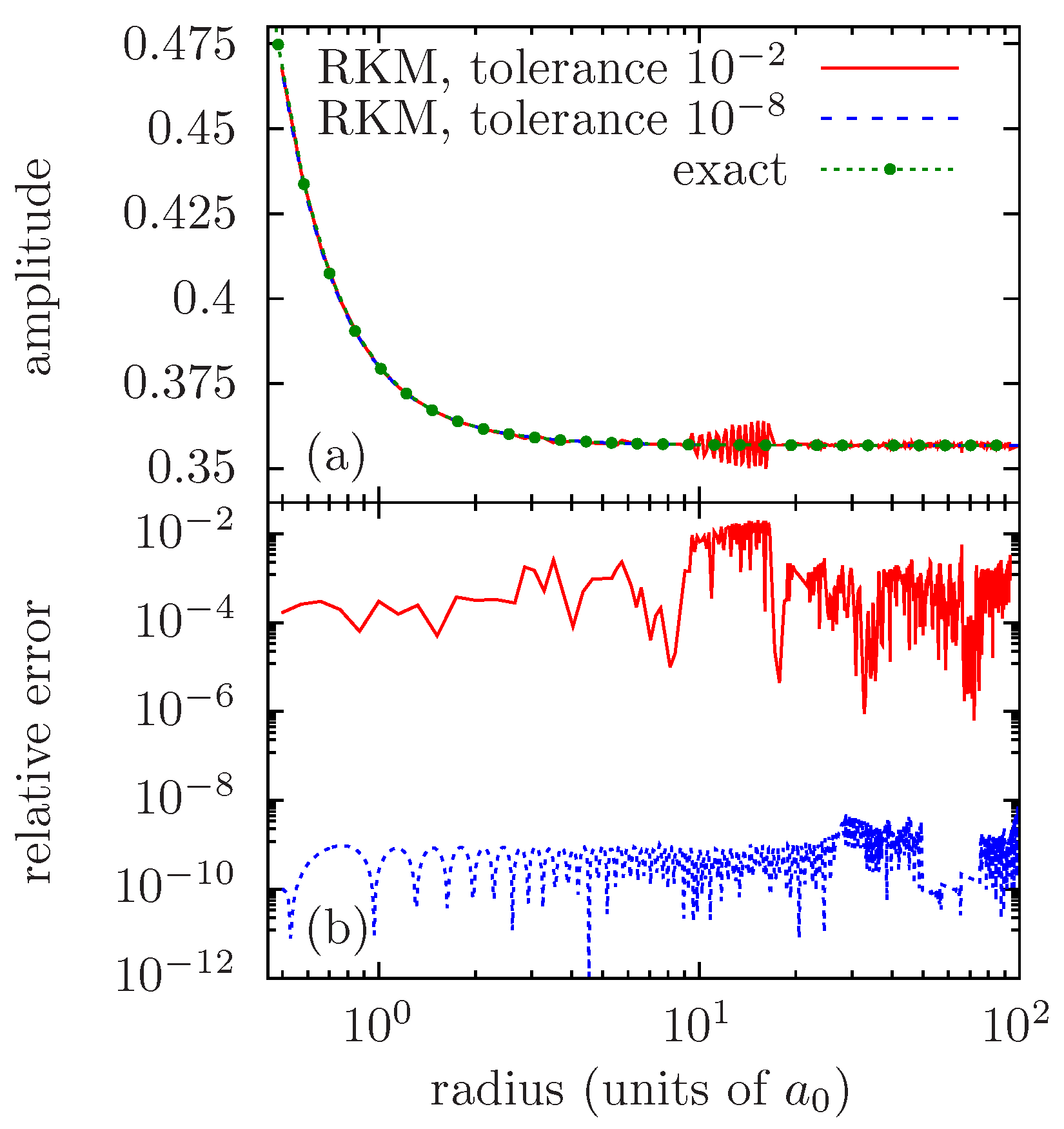
Figure 3 presents the results obtained with the RKM method on the same case as in Figure 2, with the base grid being that of Figure 2a,b (100 points, out of which 38 for the $[r_{\mathrm{match}},r_{\max }]$ interval).

Setting the tolerance to ${10}^{-2}$, one can see how the spurious solution can grow, requiring the method to refine the grid in order to correctly sample its rapid variations. In the present case, the refined grid actually has 436 points, which should be compared with the 38 points between $r_{\mathrm{match}}$ and $r_{\max }$ of the initial grid.

By decreasing the tolerance of the integration steps to ${10}^{-8}$, one may efficiently prevent the growth of numerical errors; however, this is carried out at the price of refining the grid even more. In the present case, the refined grid for tolerance ${10}^{-8}$ has 848 grid points.

The Kaps–Rentrop (KR) method [33,34] was used by Wilson et al. [5,14] to solve the amplitude equation related to the Dirac equation, which is an analogue of Equation (12). It is an adaptive mesh refinement method based on an implicit scheme.

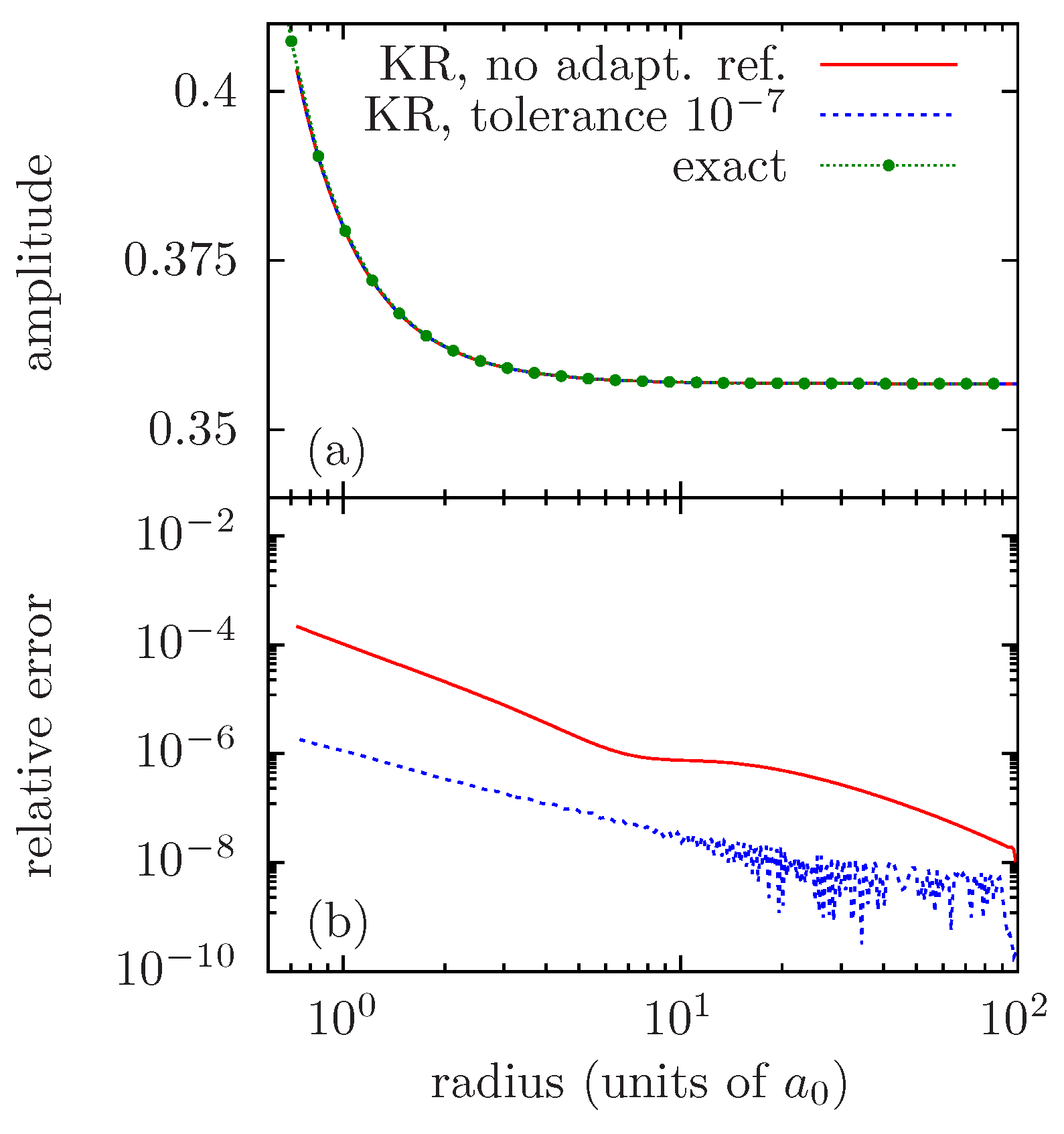
Figure 4 presents the results obtained with the KR method on the same case as in Figure 2, with the base grid being that of Figure 2c,d (1000 points, out of which 272 are for the $[r_{\mathrm{match}},r_{\max }]$ interval). We tried using the KR numerical scheme both with and without performing an adaptive grid refinement.

It may be seen in Figure 4a that the implicit scheme of the KR method seems stable over the whole region between $r_{\mathrm{match}}$ and $r_{\max }$. By directly using the base grid, i.e., performing no adaptive refinement, the KR numerical scheme yields a result of limited precision, with the maximum relative error being about ${10}^{-4}$ in this case. In order to improve precision, grid refinement has to be performed. Achieving a maximum relative error of about ${10}^{-6}$ requires setting the precision target to ${10}^{-7}$, which results in a refined grid of $\mathrm{16,221}$ points, which should be compared with the 272 points of the base grid.

The mechanism may be interpreted as follows. When propagating the numerical solution, errors accumulate, deviating the obtained solution from the slowly varying amplitude. The errors may be seen as a linear perturbation as that of Equation (29). As soon as the magnitude of these errors reaches the precision target of the method, the grid has to be refined in order to correctly describe the behavior of the perturbation, which actually has rapid variations.

A closely related issue is the sensitivity to errors on the boundary condition. Any inconsistency between the boundary condition and the value of $\theta$ can be viewed as a contribution from a rapidly varying component, which results in heavy grid refinement (see, for instance, [21], Figure 6.9, p. 115).

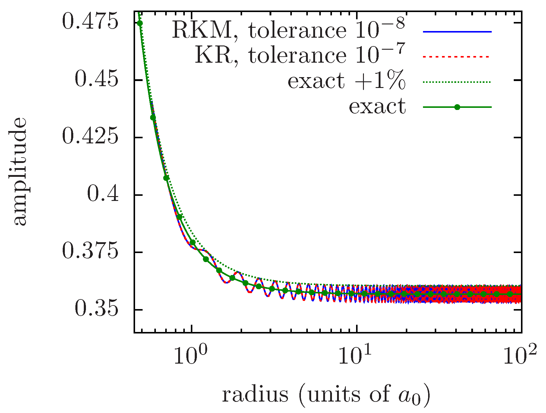
In order to illustrate the latter points, Figure 5 shows the results of the RKM and KR methods when a perturbation larger than the precision target is artificially introduced in the boundary condition. One clearly sees how these methods result in refining the grid so as to correctly sample the rapid variations of the perturbation. The same phenomenon occurs, with the much smaller perturbation induced by accumulated numerical errors, as soon as they reach the precision target.

4. Proposed Numerical Method

4.1. General Principle

In reference [20], Kiyokawa uses the following transformation, initially pointed out by Trafton (see [16], Equations (8) and (9)). By multiplying Equation (12) by $2A^{\prime }\left(r\right)$, and rearranging the terms, one can write

$$\begin{array}{c}\hfill {\displaystyle \frac{d}{dr}}\left({\left(A^{\prime }\left(r\right)\right)}^2+{\displaystyle \frac{{\theta }^2}{A{\left(r\right)}^2}}\right)+{\omega }_{k,\ell }\left(r\right){\displaystyle \frac{d}{dr}}\left(A{\left(r\right)}^2\right)=0\end{array}$$

(36)

and perform the change of function $Y\left(r\right)=A{\left(r\right)}^2$. It was noted by Kiyokawa that, if one expresses $Y^{″}\left(r\right)$ and uses Equation (12), one obtains the following relation:

$$\begin{array}{c}\hfill {\left(A^{\prime }\left(r\right)\right)}^2={\displaystyle \frac{Y^{″}\left(r\right)}{2}}+{\omega }_{k,\ell }\left(r\right)Y\left(r\right)-{\displaystyle \frac{{\theta }^2}{Y\left(r\right)}}\end{array}$$

(37)

When inserted into Equation (36), the latter relation yields a linear third-order differential equation for Y:

$$\begin{array}{c}\hfill Y^{\left(3\right)}\left(r\right)+4\omega \left(r\right)Y^{\prime }\left(r\right)+2{\omega }^{\prime }\left(r\right)Y\left(r\right)=0\end{array}$$

(38)

where $Y^{\left(3\right)}$ denotes the third derivative of Y. Kiyokawa used this linear equation in order to derive analytic results on Coulomb wavefunctions [20].

In this article, we propose to use Equation (38) for numerical calculations, instead of Equation (12). In principle, using a linear equation should exclude any coupling to spurious, rapidly varying solutions and completely solve the issue of the sensitivity to errors. We should then obtain a numerical method that is much more robust and can be applied more systematically. In particular, it should be tolerant with respect to any truncation error on the boundary condition. In this respect, it may be worth highlighting that in Equation (38), the parameter $\theta$ disappears, and the boundary condition may be defined with any multiplicative constant, as is expected and necessary for a linear equation.

Equation (38) involves the first derivative of the potential. In many cases, a solution method of the Schrödinger equation is used in an effective potential approach. Such approaches are most often based either on some analytical Ansatz for the potential, like the parametric potential approach of Klapisch [36], or on a self-consistent field model relying on some numerical solution of the Poisson equation. In both cases, the first derivatives of the potential can be easily obtained at the grid nodes, with virtually no additional cost.

In practice, the numerical scheme we propose is mostly an extension of the well-known Numerov scheme, plus an adaptation of the modified predictor–corrector scheme of Bar Shalom et al. [13].

4.2. Innermost Region

Milne’s amplitude function is singular at zero. For that reason, as is carried out in [13], we do not solve for the amplitude function close to zero. We instead solve for the wavefunction $R\left(r\right)$ using a standard Numerov scheme, propagating the solution outwards. We usually set the matching point to the radius at which some chosen fraction of the sampling limit is reached. In order to minimize the error when matching, we also set it preferably near a maximum of the wavefunction.

4.3. Intermediate Region

We recast the linear third-order equation Equation (38) under the following partial canonical form:

$$\begin{array}{cc}\hfill & \hfill Y_1^{″}\left(r\right)+4\omega \left(r\right)Y_1\left(r\right)=-2{\omega }^{\prime }\left(r\right)Y_0\left(r\right)\hfill \end{array}$$

(39)

$$\begin{array}{cc}\hfill & \hfill Y_0^{\prime }\left(r\right)=Y_1\left(r\right)\hfill \end{array}$$

(40)

where $Y_0\left(r\right)\equiv Y\left(r\right)$. We treat the first of these two equations using a standard Numerov scheme and the second one using a corollary result of the Numerov method for the derivative.

Let us consider the Taylor expansion for the q-th derivative of $Y_0$, $Y_1$:

$$\begin{array}{cc}\hfill Y_{\alpha }^{\left(q\right)}(r\pm h)=& \hfill Y_{\alpha }^{\left(q\right)}\left(r\right)\pm h{Y}_{\alpha }^{(q+1)}\left(r\right)+{\displaystyle \frac{h^2}{2}}{Y}_{\alpha }^{(q+2)}\left(r\right)\pm {\displaystyle \frac{h^3}{6}}{Y}_{\alpha }^{(q+3)}\left(r\right)+{\displaystyle \frac{h^4}{24}}{Y}_{\alpha }^{(q+4)}\left(r\right)\pm {\displaystyle \frac{h^5}{120}}{Y}_{\alpha }^{(q+5)}\left(r\right)+O\left(h^6\right)\hfill \end{array}$$

(41)

Let us consider that r is uniformly sampled: $r_n=r_{\min }+nh$. Using the Taylor expansion at $r+h$ and $r-h$, we may write

$$\begin{array}{cc}\hfill Y_{\alpha ,n+1}^{\left(q\right)}+Y_{\alpha ,n-1}^{\left(q\right)}=& \hfill 2Y_{\alpha ,n}^{\left(q\right)}+h^2{Y}_{\alpha ,n}^{(q+2)}+{\displaystyle \frac{h^4}{12}}{Y}_{\alpha ,n}^{(q+4)}+O\left(h^6\right)\hfill \end{array}$$

(42)

$$\begin{array}{cc}\hfill Y_{\alpha ,n+1}^{\left(q\right)}-Y_{\alpha ,n-1}^{\left(q\right)}=& \hfill 2h{Y}_{\alpha ,n}^{(q+1)}+{\displaystyle \frac{h^3}{3}}{Y}_{\alpha ,n}^{(q+3)}+{\displaystyle \frac{h^5}{60}}{Y}_{\alpha ,n}^{(q+5)}+O\left(h^7\right)\hfill \end{array}$$

(43)

where the n indices denote values of the functions taken at $r_n$.

First, we use Equation (42) with $\alpha =1$, $q=0$ and with $\alpha =1$, $q=2$, and we eliminate $Y_{\alpha ,n}^{\left(4\right)}$.

$$\begin{array}{cc}\hfill Y_{1,n+1}+Y_{1,n-1}=& \hfill 2Y_{1,n}+h^2{Y}_{1,n}^{″}+{\displaystyle \frac{h^2}{12}}\left(Y_{1,n+1}^{″}+Y_{1,n-1}^{″}-2Y_{1,n}^{″}\right)+O\left(h^6\right)\hfill \end{array}$$

(44)

Using Equation (39), we obtain

$$\begin{array}{c}\hfill Y_{1,n+1}\left(1+{\displaystyle \frac{h^2}{3}}{\omega }_{n+1}\right)=Y_{0,n+1}\left(-{\displaystyle \frac{h^2}{6}}{\omega }_{n+1}^{\prime }\right)+Y_{1,n}\left(2-{\displaystyle \frac{10h^2}{3}}{\omega }_n\right)+Y_{0,n}\left(-{\displaystyle \frac{10h^2}{6}}{\omega }_n^{\prime }\right)\\ \hfill +Y_{1,n-1}\left(-1-{\displaystyle \frac{h^2}{3}}{\omega }_{n-1}\right)+Y_{0,n-1}\left(-{\displaystyle \frac{h^2}{6}}{\omega }_{n-1}^{\prime }\right)+O\left(h^6\right)\end{array}$$

(45)

which corresponds to the usual Numerov scheme for a second-order inhomogeneous equation with no first-order derivative.

Then, in order to express $Y_{0,n+1}$, we use Equation (43) with $\alpha =0$, $q=0$, and with $\alpha =0$, $q=2$, and we eliminate $Y_{0,n}^{\left(3\right)}$.

$$\begin{array}{c}\hfill Y_{0,n+1}-Y_{0,n-1}=2h{Y}_{0,n}^{\prime }+{\displaystyle \frac{h^2}{6}}\left(Y_{0,n+1}^{″}-Y_{0,n-1}^{″}\right)+O\left(h^5\right)\end{array}$$

(46)

Using Equation (40) and its derivative, we obtain

$$\begin{array}{c}\hfill Y_{0,n+1}-Y_{0,n-1}=2h{Y}_{1,n}+{\displaystyle \frac{h^2}{6}}\left(Y_{1,n+1}^{\prime }-Y_{1,n-1}^{\prime }\right)+O\left(h^5\right)\end{array}$$

(47)

Let us now use Equation (43) with $\alpha =1$, $q=1$, reuse Equation (42) with $\alpha =1$, $q=2$ and eliminate $Y_{1,n}^{\left(4\right)}$:

$$\begin{array}{c}\hfill Y_{1,n+1}^{\prime }-Y_{1,n-1}^{\prime }=2h{Y}_{1,n}^{″}+{\displaystyle \frac{h}{3}}\left(Y_{1,n+1}^{″}+Y_{1,n-1}^{″}-2Y_{1,n}^{″}\right)+O\left(h^5\right)\end{array}$$

(48)

Using Equation (48) in Equation (47), and using again Equation (39) to express $Y_1^{″}\left(r\right)$, we obtain

$$\begin{array}{cc}\hfill Y_{0,n+1}\left(1+{\displaystyle \frac{h^3}{9}}{\omega }_{n+1}^{\prime }\right)=& \hfill \left(2h-{\displaystyle \frac{8h^3}{9}}{\omega }_n\right)Y_{1,n}-{\displaystyle \frac{4h^3}{9}}{\omega }_n^{\prime }{Y}_{0,n}-{\displaystyle \frac{2h^3}{9}}{\omega }_{n+1}{Y}_{1,n+1}\hfill \\ \hfill & \hfill -{\displaystyle \frac{2h^3}{9}}{\omega }_{n-1}{Y}_{1,n-1}+\left(1-{\displaystyle \frac{h^3}{9}}{\omega }_{n-1}^{\prime }\right)Y_{0,n-1}+O\left(h^5\right)\hfill \end{array}$$

(49)

Finally, we use the latter equation to eliminate $Y_{0,n+1}$ in Equation (45):

$$\begin{array}{ll}\hfill & Y_{1,n+1}\left[1+{\displaystyle \frac{h^2}{3}}{\omega }_{n+1}-\left({\displaystyle \frac{h^5}{27}}{\omega }_{n+1}^{\prime }{\omega }_{n+1}\right){\left(1+{\displaystyle \frac{h^3}{9}}{\omega }_{n+1}^{\prime }\right)}^{-1}\right]\hfill \\ \hfill & =\left(-{\displaystyle \frac{h^2}{6}}{\omega }_{n+1}^{\prime }\right){\left(1+{\displaystyle \frac{h^3}{9}}{\omega }_{n+1}^{\prime }\right)}^{-1}\hfill \\ \hfill & \phantom{=}·\left[\left(2h-{\displaystyle \frac{8h^3}{9}}{\omega }_n\right)Y_{1,n}-{\displaystyle \frac{4h^3}{9}}{\omega }_n^{\prime }{Y}_{0,n}-{\displaystyle \frac{2h^3}{9}}{\omega }_{n-1}{Y}_{1,n-1}+\left(1-{\displaystyle \frac{h^3}{9}}{\omega }_{n-1}^{\prime }\right)Y_{0,n-1}\right]\hfill \\ \hfill & \phantom{=}+Y_{1,n}\left(2-{\displaystyle \frac{10h^2}{3}}{\omega }_n\right)+Y_{0,n}\left(-{\displaystyle \frac{10h^2}{6}}{\omega }_n^{\prime }\right)+Y_{1,n-1}\left(-1-{\displaystyle \frac{h^2}{3}}{\omega }_{n-1}\right)+Y_{0,n-1}\left(-{\displaystyle \frac{h^2}{6}}{\omega }_{n-1}^{\prime }\right)\hfill \\ \hfill & \phantom{=}+O\left(h^6\right)\hfill \end{array}$$

(50)

Thus, we obtain a fully explicit expression for $Y_{1,n+1}$, relying solely on values of $Y_1$ and $Y_0$ at the points n and $n-1$. At each step, we use Equation (50) to compute $Y_{1,n+1}$ and then Equation (49) to compute $Y_{0,n+1}$. In practice, we use this numerical scheme in the inward direction. This numerical scheme is of order 6 for $Y_1$ (regular Numerov scheme), and of order 5 for $Y_0$, which is the main quantity of interest. This is to be compared with order 8 of the HPC scheme used by Bar Shalom and coauthors.

Finally, looking at Equation (50), we can see that error amplification is to be expected whenever $h^2{\omega }_{k,\ell ,n}\gtrsim 1$ or $h^2{\omega }_{k,\ell ,n}^{\prime }\gtrsim 1$, in the same way as pointed out in [13]. Although our numerical scheme is much less sensitive to the accumulation of numerical errors, we still need a complementary scheme for regions in which the grid is too coarse. A simple solution is to adapt the modified predictor–corrector scheme proposed in [13].

4.4. Outermost Region

For coarse grids, or in the outermost region of a grid of increasingly spaced points, where $h^2{\omega }_{k,\ell }\left(r\right)>1$, we propose an adaptation of the modified predictor corrector of Bar Shalom et al. [13]. The key steps are 1) using the slow variation of the amplitude to build a predictor for ($Y_1$, $Y_1^{″}$) and 2) using Equation (39) to obtain $Y_0$ from $Y_1^{\prime \prime }$, $Y_1$, thus avoiding error amplification.

Using Equation (43) with $\alpha =1$, $k=0$, we have

$$\begin{array}{c}\hfill Y_{1,n+1}-Y_{1,n-1}=2Y_{1,n}+h^2{Y}_{1,n}^{″}+O\left(h^4\right)\end{array}$$

(51)

Let us assume that $Y_1^{″}$ is varying slowly and thus is roughly equal to its average value over three successive grid points, as follows:

$$\begin{array}{c}\hfill Y_{1,n}^{″}\approx {\displaystyle \frac{1}{3}}\left(Y_{1,n-1}^{″}+Y_{1,n}^{″}+Y_{1,n+1}^{″}\right)\end{array}$$

(52)

Using this approximation in Equation (51), one obtains

$$\begin{array}{c}\hfill Z_{1,n+1}+Z_{1,n-1}=3Y_{1,n}-Z_{1,n}+O\left(h^4\right)\end{array}$$

(53)

where we define $Z_1$ as follows:

$$\begin{array}{c}\hfill Z_{1,n}=Y_{1,n}-{\displaystyle \frac{h^2}{3}}{Y}_{1,n}^{″}\end{array}$$

(54)

Equation (53) may be used as a predictor for $Z_1$:

$$\begin{array}{c}\hfill Z_{1,n+1}^{\mathrm{p}}=3Y_{1,n}-Z_{1,n}-Z_{1,n-1}+O\left(h^4\right)\end{array}$$

(55)

Let us now use Equation (43) with $\alpha =0$, $q=0$:

$$\begin{array}{c}\hfill Y_{0,n+1}-Y_{0,n-1}=2h{Y}_{0,n}^{\prime }+{\displaystyle \frac{h^3}{3}}{Y}_{0,n}^{\left(3\right)}+O\left(h^5\right)\end{array}$$

(56)

Using Equation (40) and the definition of $Z_1$, we obtain

$$\begin{array}{c}\hfill Y_{0,n+1}-Y_{0,n-1}=h\left(3Y_{1,n}-Z_{1,n}\right)+O\left(h^5\right)\end{array}$$

(57)

We finally use Equation (39) in order to obtain $Y_1$ from $Y_1^{″}$:

$$\begin{array}{cc}\hfill & \hfill Y_{1,n+1}={\displaystyle \frac{-1}{4{\omega }_{k,\ell ,n+1}}}\left(Y_{1,n+1}^{\prime \prime }+2{\omega }_{k,\ell ,n+1}^{\prime }{Y}_{0,n+1}\right)\hfill \end{array}$$

(58)

$$\begin{array}{cc}\hfill & \hfill Y_{1,n+1}={\displaystyle \frac{-1}{4{\omega }_{k,\ell ,n+1}}}\left[{\displaystyle \frac{3}{h^2}}\left(Y_{1,n+1}-Z_{1,n+1}\right)+2{\omega }_{k,\ell ,n+1}^{\prime }\left(Y_{0,n+1}+h(3Y_{1,n}-Z_{1,n})\right)\right]\hfill \end{array}$$

(59)

Because Equation (39) is linear, we obtain a linear algebraic equation for $Y_{1,n+1}$, which we readily solve analytically:

$$\begin{array}{c}\hfill Y_{1,n+1}={\left(1+{\displaystyle \frac{3}{4h^2{\omega }_{k,\ell ,n+1}}}\right)}^{-1}\left[{\displaystyle \frac{3}{4h^2{\omega }_{k,\ell ,n+1}}}{Z}_{1,n+1}-{\displaystyle \frac{{\omega }_{k,\ell ,n+1}^{\prime }}{2{\omega }_{k,\ell ,n+1}}}\left(h(3Y_{1,n}-Z_{1,n})+Y_{0,n-1}\right)\right]\end{array}$$

(60)

In the method of [13], the equation was nonlinear, and one step of a Newton method was used. When we use Equation (60), the value of $Z_{1,n+1}$ is estimated using the predictor $Z_{1,n+1}^{\mathrm{p}}$ of Equation (55). Looking at Equation (60), we clearly see that an amplification of the error on $Z_{1,n+1}^{\mathrm{p}}$ will occur when $4h^2{\omega }_{k,\ell ,n}/3\lesssim 1$.

4.5. Method Summary

To summarize, our numerical method is as follows (see also

Table 2. Summary of the numerical method proposed in the present work.

Innermost Region	Intermediate Region	Outermost Region
$[{\mathit{r}}_{\min },{\mathit{r}}_{\mathrm{match}}]$	$[{\mathit{r}}_{\mathrm{match}},{\mathit{r}}_{\mathrm{switch}}]$	$[{\mathit{r}}_{\mathrm{switch}},{\mathit{r}}_{\max }]$
$h^2{\omega }_{k,\ell }\left(r\right)<1$	$h^2{\omega }_{k,\ell }\left(r\right)<1$	$h^2{\omega }_{k,\ell }\left(r\right)>1$
Numerov scheme for $R\left(r\right)$	Equations (50) and (49)	Equations (55), (57) and (60)
Outwards	Inwards	Inwards

). From zero to a matching point, we use the usual Numerov scheme outwards, in order to solve Equation (1) for $R\left(r\right)$. The inner boundary condition that we use corresponds to a radial wavefunction regular at zero. The chosen matching point $r_{\mathrm{match}}$ is near the point at which some fraction of the sampling limit is reached, preferably close to a maximum of $R\left(r\right)$.

We then use Equations (55), (57) and (60) to propagate the solution inwards, starting from the outer boundary condition, until reaching a point where $h^2{\omega }_n\lesssim 1$. The outer boundary condition is given by Equation (15), with R, Q given by Equations (22) and (23).

In the region where $h^2{\omega }_n\lesssim 1$, we use Equations (49) and (50) to propagate the solution further inwards, up to the matching point.

Matching is performed in order to normalize the inner part of $R\left(r\right)$ according to the outer boundary condition, as well as to determine the phase at the matching radius. The phase function is subsequently obtained by integrating the function $\varphi \left(r\right)-kr$ outwards using, for instance, Simpson’s rule.

5. Test of the Method

We tested the present method using linear grids, quadratic grids, exponentially spaced grids, and mixed linear–exponential grids. The relations between the radius $\rho$ in these grids and the parameter r which is uniformly sampled are recalled in

Table 3. Change of the variables and functions (f) corresponding to various grids.

Grid Type	Change of Variable	Function f of Equation (61)
Linear	$r=\rho$	1
Quadratic	$r=\sqrt{\rho }$	${\rho }^{1/4}$
Exponential	$r=ln\left(\rho \right)$	$\sqrt{\rho }$
Exponential-linear	$r=ln\left(\rho \right)+a\rho$	$\sqrt{{\displaystyle \frac{\rho }{1+a\rho }}}$

. Together with the change of variable from $\rho$ to r, we perform the following change of function $A\left(\rho \right)\to \widehat{A}\left(r\right)$, which leaves Equations (1), (12) and (38) invariant:

$$\begin{array}{c}\hfill \widehat{A}\left(\widehat{r}\left(\rho \right)\right)=A\left(\rho \right)/f\left(\rho \right)\end{array}$$

(61)

The relevant functions $f\left(\rho \right)$ for each grid are also given in Table 3.

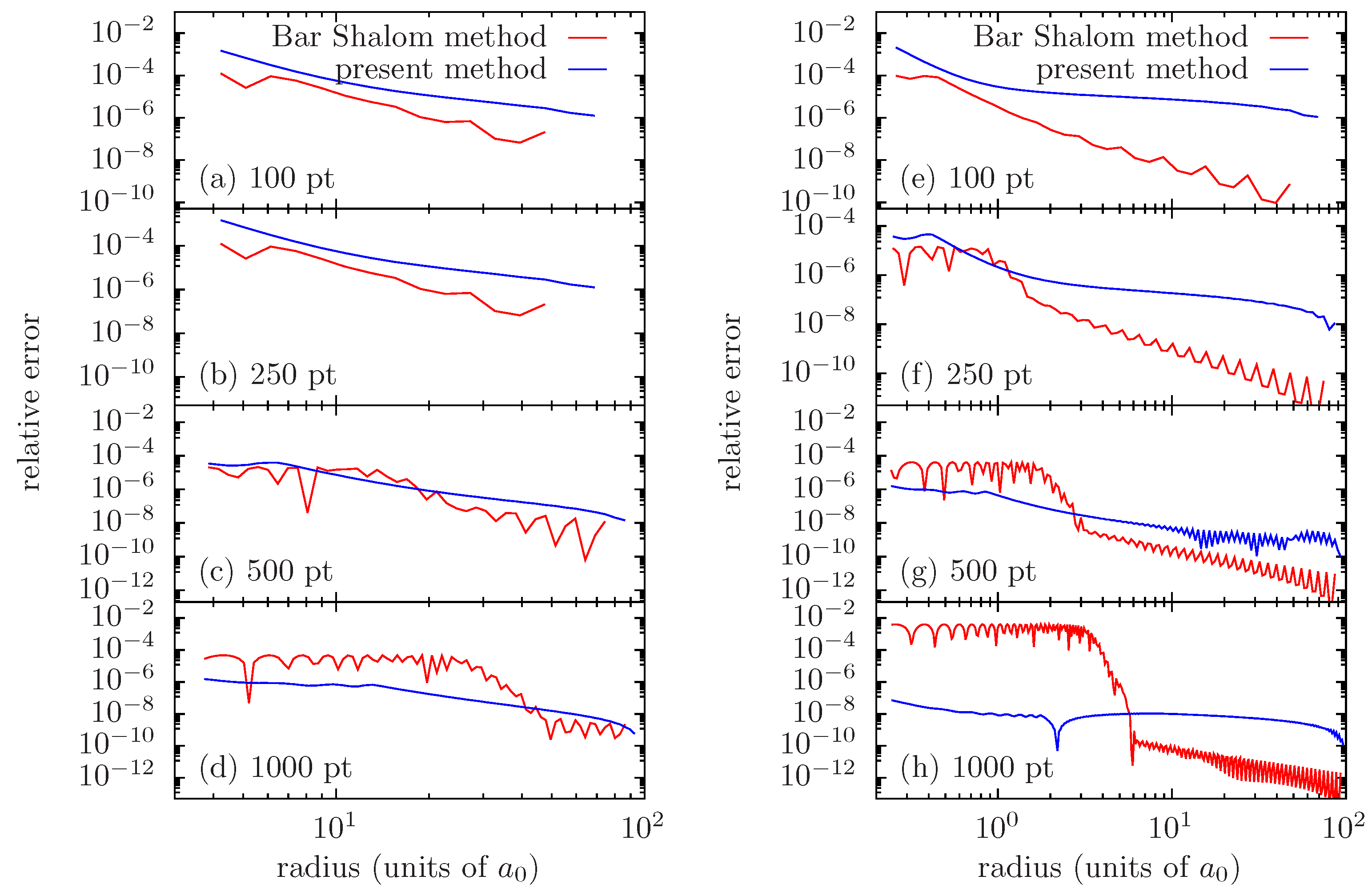
Figure 6 presents the relative error on the amplitude function obtained with our method, compared to that of [13], in the case of zero potential, for $\ell =2$, $k=1a_0^{-1}$ and $15a_0^{-1}$. In order to remain as close as possible to reference [13], we perform this comparison using an exponentially spaced grid, varying the number of grid points. We also set the matching point to be located not farther than the first maximum of $R\left(r\right)$.

Errors in the outermost region seem systematically larger with the present method than with the method of [13]. This may indicate that the approximation of Equation (52) is less justified for $Y^{\left(3\right)}\left(r\right)$ than it is for $A^{″}\left(r\right)$. However, the largest contribution to the numerical errors stems from error accumulation in the intermediate region, where the amplitude varies more significantly. Consequently, we do not consider the numerical scheme used in the outermost region as a limiting factor for our method.

Using a coarse grid (see Figure 6a,e), for which the method of [13] performs well, error growth in the intermediate region is stronger with our fifth-order scheme than with the HPC scheme, which is of the eighth order. This is fully expected.

Considering finer grids (see Figure 6b–d,f–h), one clearly sees the effect of the spurious component that appears with the method of [13], which puts a lower bound on the precision that may be achieved and ultimately ruins the solution. On the contrary, the present method exhibits a continuous improvement of precision, when one refines the grid. Beyond some grid refinement, it may become relevant to improve the solution in the outermost region. This can be carried out as suggested in [13], by making some iterative steps after applying the modified predictor–corrector scheme.

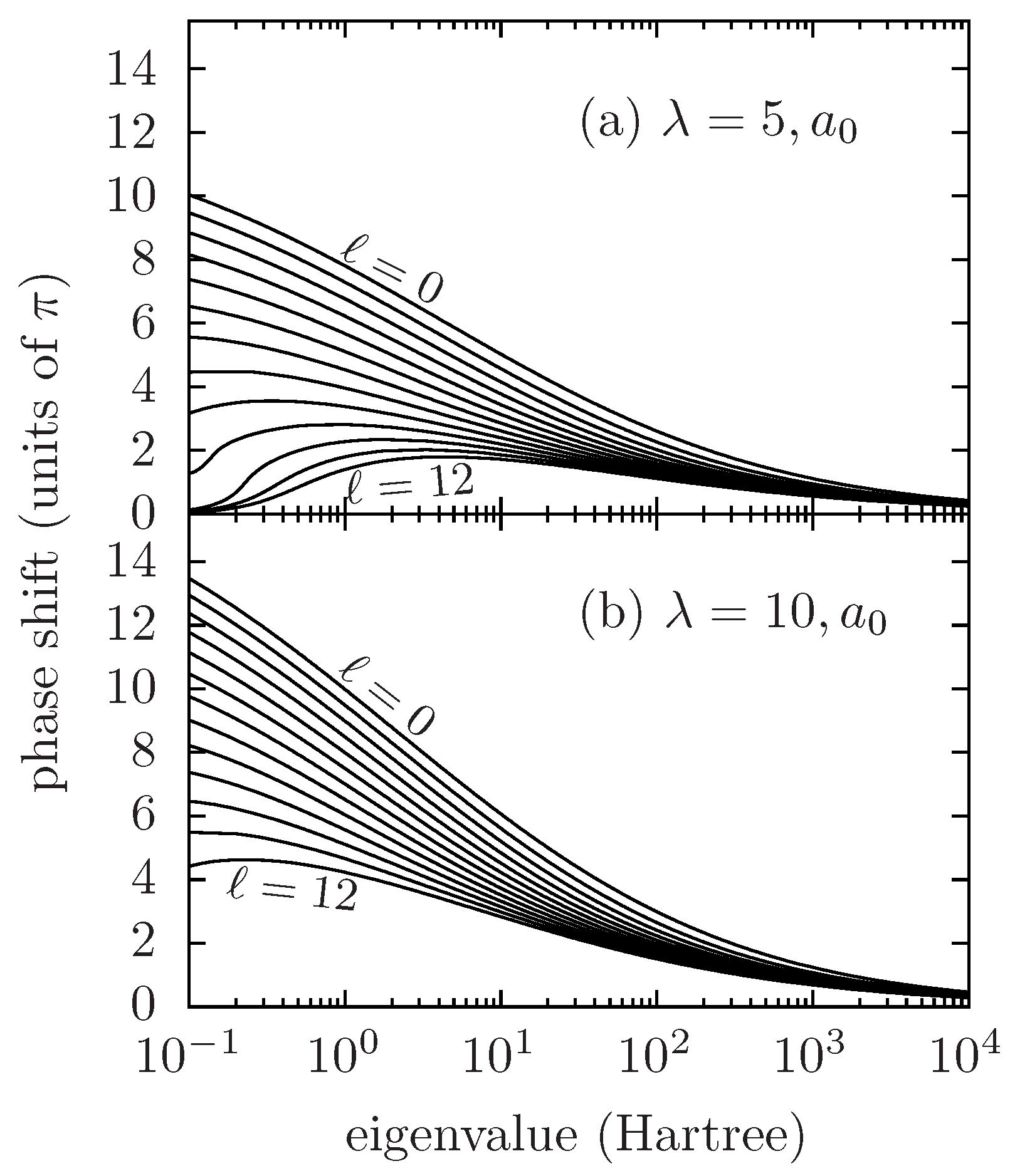
As an example of the systematic application of the present numerical method, we present, in Figure 7, the phase shifts as functions of eigenvalue (i.e., orbital energy) for two fully screened Coulomb potentials with $Z=26$, decay length $\lambda =5$ and $10a_0$, for an orbital number ℓ ranging from 0 to 12. These curves were obtained using the present method on an exponentially spaced grid of 1000 points, spanning from ${10}^{-6}{a}_0$ to $100a_0$. Using the Milne PA representation with the present numerical method allows one to compute phase shifts for arbitrarily high eigenvalues while keeping this relatively coarse radial grid. Recovering comparable results from a computation of the oscillatory wavefunction $R\left(r\right)$ on the same range of radii and energies typically requires a radial grid with a few hundred thousand points.

The computation of wavefunctions for a partially screened potential, i.e., a potential having a Coulomb tail $-Z^{*}/r$, can be carried out according to the same method, using the Coulomb wavefunctions in the boundary condition instead of Bessel functions (see Equations (22), (23) and (15)). One would then be interested in finding the phase shifts with respect to the Coulomb wavefunctions related to the asymptotic charge $Z^{*}$.

6. Conclusions

In the present article, we address the challenges inherent in solving Milne’s amplitude equation, a critical step in accurately modeling atomic processes in plasmas. We identified limitations in existing numerical methods, such as the predictor–corrector scheme of Bar Shalom et al. [13] and adaptive grid refinement techniques, stemming from their proneness to let spurious, rapidly varying solutions emerge. To overcome these limitations, we developed a fully explicit numerical method based on the linear equation derived by Kiyokawa [20]. This approach effectively eliminates the coupling to spurious solutions, resulting in a more robust scheme which allows for a systematic improvement in accuracy when grid’s resolution is increased. To outline an indication of the potential of this method, we illustrate its application with regard to the calculation of phase shifts. Applications of this method to the calculation of atomic cross-sections will be pursued in our subsequent work, notably elaborating from the previous works on collisional cross-sections [13] and free–free photoabsorption cross-sections [14].

References

1. Blenski, T.; Piron, R.; Caizergues, C.; Cichocki, B. Models of atoms in plasmas based on common formalism for bound and free electrons. High Energy Density Phys. 2013, 9, 687–695. [Google Scholar] [CrossRef]
2. Piron, R. Atomic Models of Dense Plasmas, Applications, and Current Challenges. Atoms 2024, 12, 26. [Google Scholar] [CrossRef]
3. Piron, R. Atoms in Dense Plasmas: Models, Applications, and Current Challenges. Habilitation Thesis, Sorbonne Université, Paris, France, 2024. [Google Scholar] [CrossRef]
4. Liberman, D.A. Self-consistent field model for condensed matter. Phys. Rev. B 1979, 20, 4981–4989. [Google Scholar] [CrossRef]
5. Wilson, B.; Sonnad, V.; Sterne, P.; Isaacs, W. Purgatorio—A new implementation of the Inferno algorithm. J. Quant. Spectrosc. Radiat. Transf. 2006, 99, 658–679. [Google Scholar] [CrossRef]
6. Piron, R.; Blenski, T. Variational-average-atom-in-quantum-plasmas (VAAQP) code and virial theorem: Equation-of-state and shock-Hugoniot calculations for warm dense Al, Fe, Cu, and Pb. Phys. Rev. E 2011, 83, 026403. [Google Scholar] [CrossRef]
7. Piron, R.; Blenski, T. Average-atom model calculations of dense-plasma opacities: Review and potential applications to white-dwarf stars. Contrib. Plasma Phys. 2018, 58, 30–41. [Google Scholar] [CrossRef]
8. Shannon, C. Communication in the Presence of Noise. Proc. IRE 1949, 37, 10–21. [Google Scholar] [CrossRef]
9. Starrett, C.E.; Shaffer, N.R. Average-atom model with Siegert states. Phys. Rev. E 2023, 107, 025204. [Google Scholar] [CrossRef]
10. Batishchev, P.A.; Tolstikhin, O.I. Siegert pseudostate formulation of scattering theory: Nonzero angular momenta in the one-channel case. Phys. Rev. A 2007, 75, 062704. [Google Scholar] [CrossRef]
11. Milne, W.E. The numerical determination of characteristic numbers. Phys. Rev. 1930, 35, 863–867. [Google Scholar] [CrossRef]
12. Goldstein, M.; Thaler, R.M. Bessel Functions for Large Arguments. Math. Tables Other Aids Comput. 1958, 12, 18–26. [Google Scholar] [CrossRef]
13. Bar-Shalom, A.; Klapisch, M.; Oreg, J. Phase-amplitude algorithms for atomic continuum orbitals and radial integrals. Comput. Phys. Commun. 1996, 93, 21–32. [Google Scholar] [CrossRef]
14. Wilson, B.; Sonnad, V.; Sterne, P.; Isaacs, W. Improvements in the phase-amplitude method for calculating free-free gaunt factors and spherical bessel function of high angular momentum. J. Quant. Spectrosc. Radiat. Transf. 2003, 81, 499–512. [Google Scholar] [CrossRef]
15. Seaton, M.J.; Peach, G. The Determination of Phases of Wave Functions. Proc. Phys. Soc. 1962, 79, 1296. [Google Scholar] [CrossRef]
16. Trafton, L. A rapid numerical solution to the radial Schroedinger equation in the oscillatory region. J. Comput. Phys. 1971, 8, 64–72. [Google Scholar] [CrossRef]
17. Rawitscher, G. A spectral Phase–Amplitude method for propagating a wave function to large distances. Comput. Phys. Commun. 2015, 191, 33–42. [Google Scholar] [CrossRef]
18. Bar-Shalom, A.; Oreg, J.; Klapisch, M. Non-LTE Superconfiguration Collisional Radiative Model. J. Quant. Spectrosc. Radiat. Transf. 1997, 58, 427–439. [Google Scholar] [CrossRef]
19. Bar-Shalom, A.; Klapisch, M.; Oreg, J. HULLAC, an integrated computer package for atomic processes in plasmas. J. Quant. Spectrosc. Radiat. Transf. 2001, 71, 169–188. [Google Scholar] [CrossRef]
20. Kiyokawa, S. Exact solution to the Coulomb wave using the linearized phase-amplitude method. AIP Adv. 2015, 5, 087150. [Google Scholar] [CrossRef]
21. Piron, R. Variational Average-Atom in Quantum Plasmas (VAAQP). Ph.D. Thesis, École Polytechnique, Palaiseau, France, 2009. [Google Scholar]
22. Good, R.H. The Generalization of the WKB Method to Radial Wave Equations. Phys. Rev. 1953, 90, 131–137. [Google Scholar] [CrossRef]
23. Rosen, M.; Yennie, D.R. A Modified WKB Approximation for Phase Shifts. J. Math. Phys. 1964, 5, 1505–1515. [Google Scholar] [CrossRef]
24. Wald, S.S.; Lu, P. Modified WKB approximation for phase shifts of an attractive singular potential. Phys. Rev. D 1974, 10, 3434–3440. [Google Scholar] [CrossRef]
25. Stein, J.; Ron, A.; Goldberg, I.B.; Pratt, R.H. Generalized WKB approximation to nonrelativistic normalizations and phase shifts in a screened Coulomb potential. Phys. Rev. A 1987, 36, 5523–5529. [Google Scholar] [CrossRef] [PubMed]
26. Calogero, F. A novel approach to elementary scattering theory. Il Nuovo Cimento 1963, 27, 261–302. [Google Scholar] [CrossRef]
27. Calogero, F. Variable Phase Approach to Potential Scattering. In Mathematics in Science and Engineering; Elsevier: Amsterdam, The Netherlands, 1967; Volume 35, ISBN 978-0121555504. [Google Scholar]
28. Green, A.E.S.; Rio, D.E.; Schippnick, P.F.; Schwartz, J.M.; Ganas, P.S. Analytic Phase Shifts for Yukawa Potentials. Int. J. Quantum Chem. 1982, 16, 331–343. [Google Scholar] [CrossRef]
29. Blenski, T.; Ligou, J. An improved shooting method for one-dimensional schrödinger equation. Comput. Phys. Commun. 1988, 50, 303–311. [Google Scholar] [CrossRef]
30. Nikiforov, A.F.; Novikov, V.G.; Uvarov, V.B. Quantum-Statistical Models of Hot Dense Matter; Birkhauser: Basel, Switzerland, 2005; ISBN 978-3764321833. [Google Scholar]
31. Abramowitz, M.; Stegun, I.A. Handbook of Mathematical Functions with Formulas, Graphs, and Mathematical Tables; Dover Publication, Inc.: New York, NY, USA, 1965; ISBN 978-0486612720. [Google Scholar]
32. Hamming, R.W. Numerical Methods for Scientists and Engineers; Dover Publication, Inc.: Garden City, NY, USA, 1986; ISBN 978-0486652412. [Google Scholar]
33. Kaps, P.; Rentrop, P. Generalized Runge-Kutta Methods of Order Four with Stepsize Control for Stiff Ordinary Differential Equations. Numer. Math. 1979, 33, 55–68. [Google Scholar] [CrossRef]
34. Press, W.H.; Teukolsky, S.A.; Vetterling, W.T.; Flannery, B.P. Numerical Recipes, The Art of Scientific Computing; Cambridge University Press: Cambridge, UK, 2007; ISBN 978-0521880688. [Google Scholar]
35. Merson, R.H. An operational method for the study of integration processes. In Proceedings of the Conference Data Processing and Automatic Computing Machines, Weapons Research Establishment Salisbury, Salisbury, Australia, 3–8 June 1957; pp. 110-1–110-26. [Google Scholar]
36. Klapisch, M. A program for atomic wavefunction computations by the parametric potential method. Comput. Phys. Commun. 1971, 2, 239–260. [Google Scholar] [CrossRef]
Figure 1. Radial wavefunction and amplitude function for values = 2 and k = 1 in three distinct potentials: zero potential (a), Yukawa potential Z e r / λ / r with Z = 26 , λ = 10 (b), and pure Coulomb potential Z / r with Z = 26 (c).
Atoms 13 00057 g001
Figure 2. Radial wavefunction and amplitude function (a,c), with the corresponding relative errors (b,d) obtained with the method of [13] for the case of zero potential, = 2 , k = 5 a 0 1 , using an exponentially spaced grid spanning from 10 4 to 10 2 a 0 . The exact solutions are shown with green dots and dashed line. Comparison of results obtained using grids of 100 (a,b) and 1000 (c,d) grid points in total, respectively. The 100-point grid has 38 steps between r match and r max , whereas the 1000-point grid has 272 steps in this region.
Atoms 13 00057 g002
Figure 3. Amplitude function (a), with the corresponding relative error (b) obtained with the Runge–Kutta–Merson adaptive refinement method, for the case of zero potential, = 2 , k = 5 a 0 1 , using an initial grid of 100 exponentially spaced points, spanning from 10 4 to 10 2 a 0 . The presented results correspond to precision targets (or tolerances) of 10 2 and 10 8 . In the present case, the corresponding refined grids have 436 and 848 grid points between r match and r max , respectively. The initial grid has 38 steps in this region.
Atoms 13 00057 g003
Figure 4. Amplitude function (a), with the corresponding relative error (b) obtained with the Kaps–Rentrop method, for the case of zero potential, = 2 , k = 5 a 0 1 , using a exponentially spaced base grid of 1000 points, spanning from 10 4 to 10 2 a 0 . We present results obtained with and without adaptive grid refinement. In the present case, the refined grid corresponding to the precision target of 10 7 has 16,221 grid points between r match and r max . The initial grid has 272 steps in this region.
Atoms 13 00057 g004
Figure 5. Amplitude functions obtained with the Runge–Kutta–Merson and Kaps–Rentrop methods, respectively, for the case of zero potential, = 2 , k = 5 a 0 1 , artificially introducing a 1% error on the boundary condition. Results shows rapid oscillations due to the spurious component of the solution.
Atoms 13 00057 g005
Figure 6. Relative error on the amplitude function obtained with the Bar Shalom method and with the present method. Case of zero potential, for = 2 , k = 1 a 0 1 (ad) and k = 15 a 0 1 (eh) using a exponentially spaced grid spanning from 10 6 to 10 2 a 0 with 100 (a,e), 250 (b,f), 500 (c,g), and 1000 (d,h) points, respectively. The error is shown only from the matching radius to the grid’s outer boundary.
Atoms 13 00057 g006
Figure 7. Scattering phase shifts calculated using the present method for two cases of fully screened Coulomb potential Z e r / λ / r with Z = 26 , λ = 5 a 0 (a) and 10 a 0 (b) for eigenvalues k 2 / 2 ranging from 10 1 to 10 4 Hartree and an orbital quantum number ranging from 0 to 12.
Atoms 13 00057 g007