1. Introduction
Magnetic field sensing is crucial for understanding many concepts of fundamental and applied sciences, with different applications in the fields of quantum metrology, space research, and navigation, among others. Conventional magnetic sensors such as fluxgate magnetometers [
1] and Hall-effect sensors utilize classical electromagnetic coupling between the field and the probe. These devices offer a detection range from 1 nT to 10
7 nT and a sensitivity limited to 1 nT/√Hz. In contrast, quantum magnetic sensors such as the SQUIDs [
2] (Superconducting Quantum Interference Device), provide much higher sensitivities for measuring weak magnetic fields, with sensitivities around 1 fT/√Hz. However, they are constrained by the need for complex and costly cryogenic systems and limited spatial resolution [
3,
4,
5,
6].
In the past 20 years, atomic magnetic sensing methods [
7,
8] based on neutral atoms have emerged as a compact, non-cryogenic alternative for achieving sub-femtotesla sensitivity in weak magnetic fields. Thermal atomic magnetic sensing techniques operate at room temperature and use atomic vapors to measure magnetic fields, achieving sensitivities down to about 1 fT/√Hz. However, they are limited by thermal noise and Doppler broadening due to high atomic velocities, affecting their precision and spatial resolution [
3,
9,
10].
Cold or ultra-cold systems [
11] improve on this by using cold atomic ensembles or Bose–Einstein condensates (BECs) [
12,
13,
14], which have significantly reduced thermal velocities. This reduction minimizes thermal noise and sharpens resonance signals, resulting in much higher sensitivities, often reaching the sub-femtotesla range, and higher spatial resolution. Their ability to manipulate quantum states and maintain longer coherence times makes cold atomic magnetometers superior for precise magnetic field measurements. However, these experiments involve sophisticated setups and detailed protocols and depend upon imaging of the atomic cloud. Additionally, the achieved sensitivities often fall short of those provided by thermal atomic magnetic sensing methods, and the magnetic field is measured indirectly. Consequently, the practical application of cold atomic magnetic sensing techniques remained limited [
3,
14,
15,
16].
In this paper, we demonstrate and characterize quantum sensing measurements to observe spatially resolved magnetic field variations using cesium-133 atoms cooled to approximately 3 µK. The cesium fountain atomic clock measures the clock transition frequency of 9,192,631,770 Hz with high precision [
17,
18,
19]. To ensure accurate measurements of this frequency, the degeneracy of the hyperfine state must be removed. Thus, after laser cooling, a hyperfine state sensitive to the magnetic field is created through a uniform magnetic field produced by a solenoid, enabling precise mapping of magnetic field variations. The cold cesium atoms are launched using frequency detuned vertical laser beams. During their ballistic flight, the atoms interact with the microwaves, reach a height, and then fall back under gravity. As they exit the flight tube, two horizontal detection beams are turned on, and the fluorescence signal is collected by large-area photodiodes and is monitored on a PC via a data acquisition (DAQ) card. The Ramsey method of interrogation is employed to achieve high-resolution atomic transition frequency measurements with reduced Doppler broadening and high sensitivity to phase differences. The Direct digital synthesizer (DDS) frequency is scanned to produce Ramsey fringes for precise atomic transition frequency measurements. Ramsey fringes for magnetic field sensitive states are observed at various launch heights of the atomic cloud. The central fringe frequency varies with launch height, allowing the creation of a map of the magnetic field as a function of height by deconvoluting the fringe shift data. Hence, we trace the magnetic field within the ultrahigh vacuum using cesium atoms as quantum magnetic sensors, providing spatially resolved measurements of magnetic field variations across the experimental region. In a shielded environment, we achieve a magnetic field sensitivity of approximately 550 pT/√Hz.
2. Experimental Setup
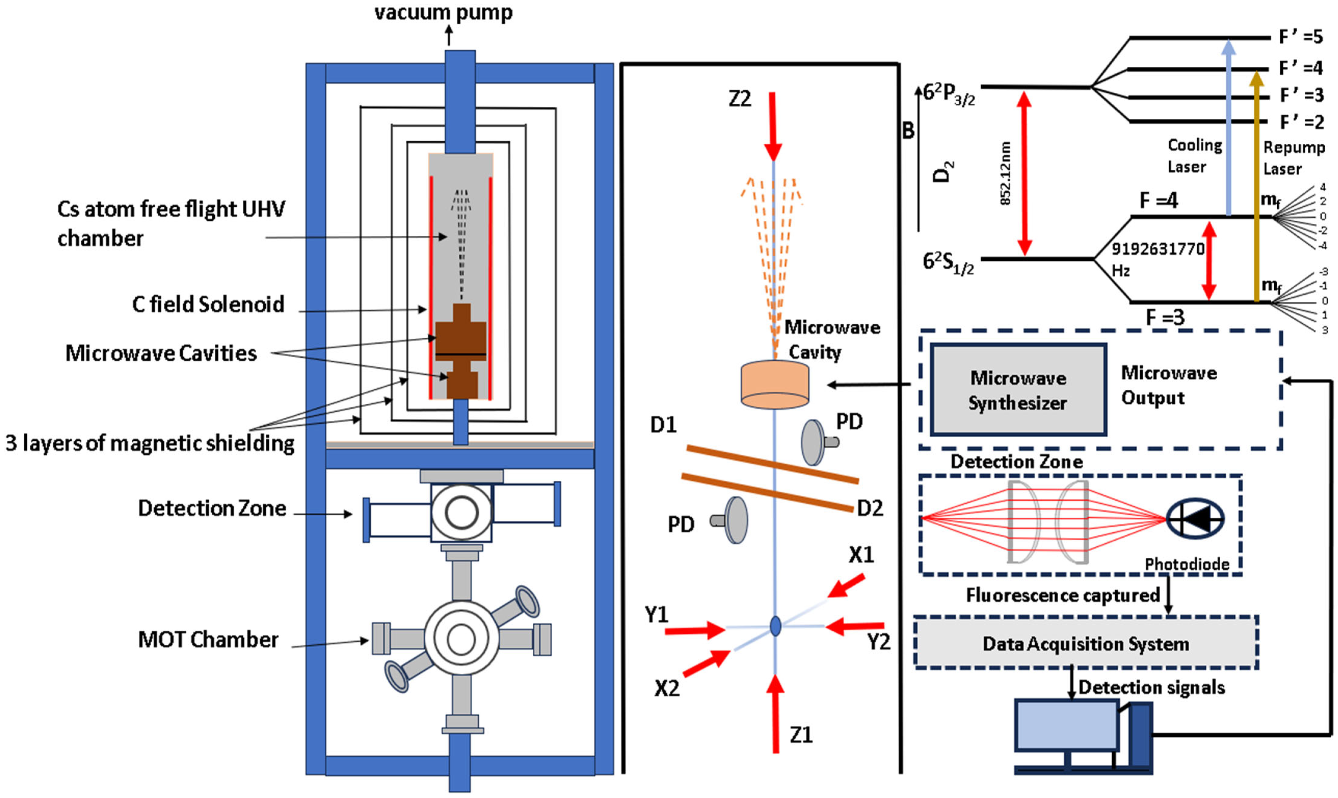
The system, as shown in
Figure 1, features a magneto-optical trap (MOT) with a (0, 0, 1) geometry, aligned along the
Z-axis, for cooling and launching the cesium atoms. The cesium atoms are cooled in a 3D MOT and then further cooled in optical molasses (OM) inside an octagonal stainless-steel chamber. A quadrupole magnetic field gradient of 6 G/cm is produced in the trapping region by two coils, each with a radius of 75 mm and 100 turns in an anti-Helmholtz configuration. Furthermore, the background magnetic field at the atoms’ location is compensated for by three pairs of Helmholtz coils (pointing in the X, Y, and Z directions) surrounding the MOT. A temperature-controlled cold finger with a Cs ampoule connected to the MOT chamber is the source of Cs [
18,
20].
The cooling process includes an Extended cavity diode laser (ECDL at 852 nm) in Littrow mode which is frequency locked to a cesium D2 line [crossover peak of 133Cs 6 2S1/2 (F = 4) → 6 2P3/2 (F′ = 4 and 5)], generated by high-resolution saturated absorption spectroscopy. The laser output is amplified by a tapered amplifier system (Toptica TA Pro) and is divided into four horizontal cooling beams with an average intensity of 10 mW cm−2 per MOT beam and two vertical beams with an average intensity of 3 mW cm−2 per beam. Besides the cooling beams, the optical setup provides two beams for detection (D1, D2) with average intensity of 2 mW cm−2 per beam. A re-pumping laser (ECDL at 852 nm) is tuned and locked to the transition 133Cs 6 2S1/2 (F = 3, mf = 0) → 6 2P3/2 (F′ = 4, mf = 0) by high-precision laser saturated absorption spectroscopy. The output beam is split and mixed with one of the cooling beams, Y2, and a detection beam, D2, with average intensity of 5 mW cm−2. Acousto-optic modulators (AOMs) in a double-pass configuration are used to regulate the frequency and intensity of the cooling beams. Quick switching between lasers is achieved using mechanical shutters and computer-controlled AOMs. The mechanical shutters feature a rise time of approximately 500 µs and a fall time of approximately 400 µs, enabling efficient and precise control over the laser beams.
The atomic trap is monitored via destructive absorption imaging and real-time fluorescence imaging. Directly above the MOT is the detection chamber, and above it is the aluminium flight tube, enclosed within three layers of mu metal magnetic shield. Two horizontal, parallel detection beams are spaced 45 mm vertically apart and are individually formed into 10 mm squares using apertures. The fluorescence collector ensembles for the atoms in the two states F = 4 and F = 3 are positioned perpendicular to the detection laser beams. Each ensemble comprises of a pair of achromatic plano-convex imaging lenses (50 mm diameter and 75 mm focal length), as shown in
Figure 1, arranged back-to-back, focusing the light onto a large-area silicon photodiode (10 mm square) [
18,
20].
Within the flight tube, there are two microwave cavities: the Ramsey cavity and the state-selection cavity. The center of the Ramsey cavity is located 52.5 cm above the trap center. The source for the microwave interrogation is a synthesizer that has been designed in collaboration with PTB, Germany. A uniform C-field which lifts the degeneracy of the energy states and splits them into 2F + 1 Zeeman levels for accurate measurement of the clock transition frequency is produced using a solenoid with 320 turns wound on a former with a diameter of 235 mm and length of 640 mm, ensuring a stable magnetic environment and minimizing uncertainties in frequency evaluation. The C-field generates a magnetic field of 104 nT. The solenoid is placed inside the innermost mu metal shield and, together with three additional compensation coils at the top and bottom, produces a homogeneous C-field of about 104 nT over the drift region. Two 55 l/s ion pumps on the top of the vacuum assembly keep the pressure inside the flight tube at 8 × 10
−8 Pa [
18].
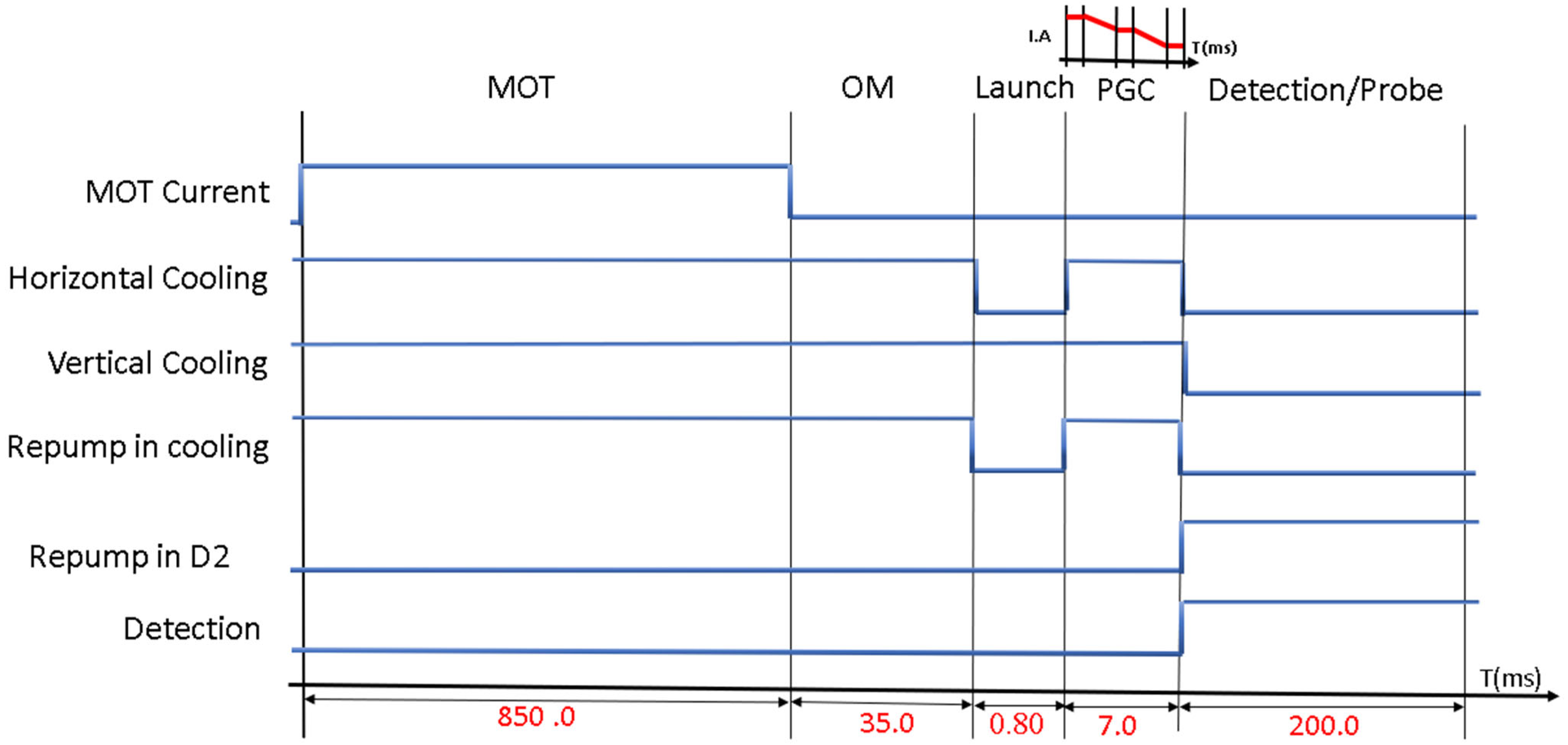
The timing sequence generation [
18,
20] proceeds as sketched in
Figure 2 to run the process from MOT loading to polarization gradient cooling and measurement of detection signal. Initially, the cooling laser is frequency detuned by approximately −2Γ, where Γ = 5.2 MHz [
21], and atoms are typically loaded for up to 850 ms in the MOT. The atomic cloud is then further cooled by optical molasses for 35 ms. The atoms are then launched using moving molasses and cooled further with Polarization gradient cooling (PGC) for 7 ms, which brings the atoms’ temperature down to approximately 3 µk. Up to 10
7 atoms are trapped in the PGC phase. During this phase, the intensity of the cooling beams is gradually reduced while the detuning is incrementally increased, achieved through a frequency ramp as shown in
Figure 2. After cooling, all laser beams are turned off, and the atoms are launched by applying frequency-detuned vertical laser beams, with the upward directed beam tuned to a frequency
and the downward beam tuned to a frequency
, imparting an initial velocity that causes the atoms to ascend to a height H
m and then fall back under gravity.
During this ballistic flight, the atoms interact with two microwave (π/2) pulses in the Ramsey interrogation process. The first pulse excites the cesium atoms from the ground state into a superposition of the F = 3 and F = 4 states. After a delay, the second pulse allows the atoms to interact with the microwave field again, leading to an interference pattern known as Ramsey fringes. Thus, the atomic cloud interacts with the Ramsey cavity twice, and the time interval between these pulses determines the coherence and phase of the superposition, producing the observed Ramsey fringe pattern. As the atoms exit the flight tube, detection beams are turned on. Photodiodes capture the fluorescence signal from the falling atoms within a detection window of 200 ms and transmit it to the PC through a data acquisition (DAQ) card. Microcontroller-based cards regulate the entire timing sequence, and a LabVIEW application handles data processing and acquisition.
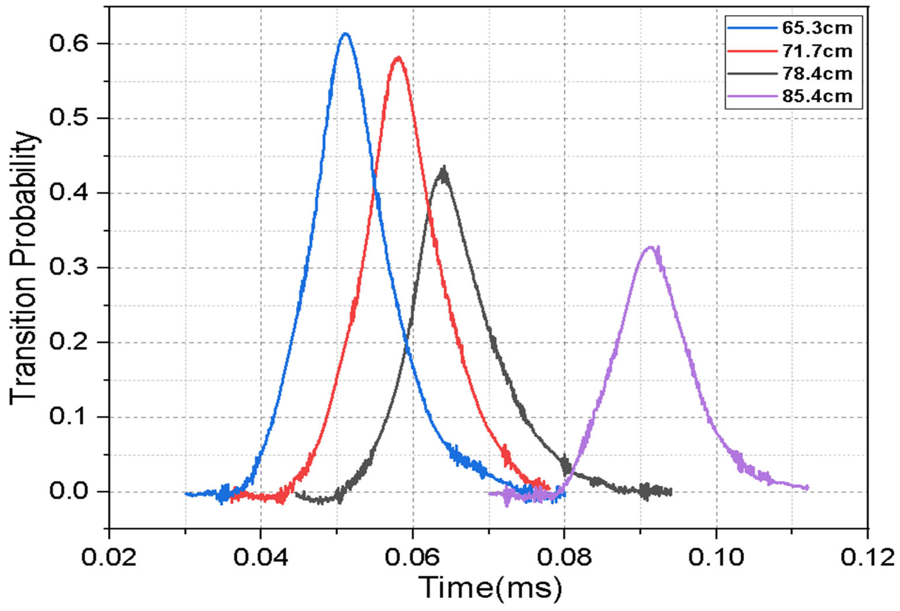
Atoms can be launched to various heights by changing the launch frequency, and the time of arrival (time between the launch and when the atomic cloud) is detected. Higher launch velocities lead to greater heights and longer time of arrival. As launch height increases, the atomic cloud expands more, resulting in greater atom loss when passing through the microwave cavities. A cooler and more tightly confined cesium cloud can be launched higher with less expansion.
Figure 3 shows the return signals with increasing launch velocities and thus increasing launch heights and times of arrivals.
3. Results and Discussion
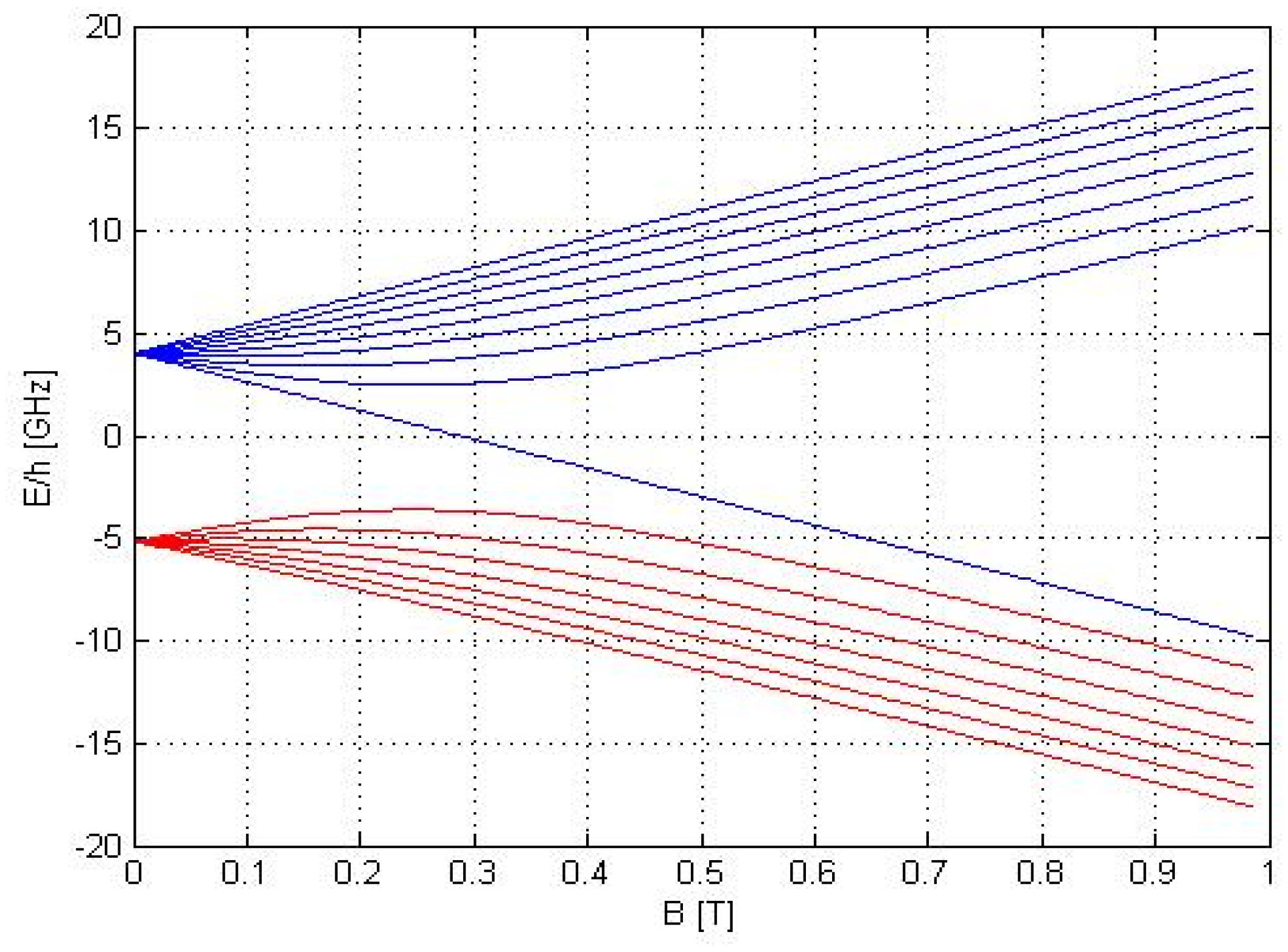
To precisely measure the magnetic field strength inside the flight tube, we utilize the linear Zeeman frequency shift of magnetically sensitive transitions
since, the clock transition
is not very sensitive to the magnetic field changes and has a small frequency shift proportional to
. In general, Zeeman shift is measured by measuring the shift in the central fringe for the
transition which has a linear dependence on the magnetic field B. If we denote the difference between the
transition and the
transition as
and neglect higher orders, the 2nd order Zeeman shift is given by the Breit–Rabi formula (solution given in
Figure 4) as follows [
19,
22]:
where
= 2.00254032 and
= −0.00039885395 are Lande
-factors of the electron and the nucleus,
µB = 9.27400899 × 10
−24 J. T
−1 is the Bohr magnetron [
21],
ν0 is the clock transition frequency
, brackets ⟨ ⟩ indicate a time-averaged value over the interaction time
T, and
is the mean squared magnetic field averaged over the flight region above the microwave cavity. When the C-field is inhomogeneous,
is given by the following:
where
is the variance of B along the atomic trajectory.
Using Equations (1)–(4), the second-order Zeeman shift is given by the following:
Further, the uncertainty of the 2nd order Zeeman shift is given by the temporal instability of
:
where
is the temporal variation of
.
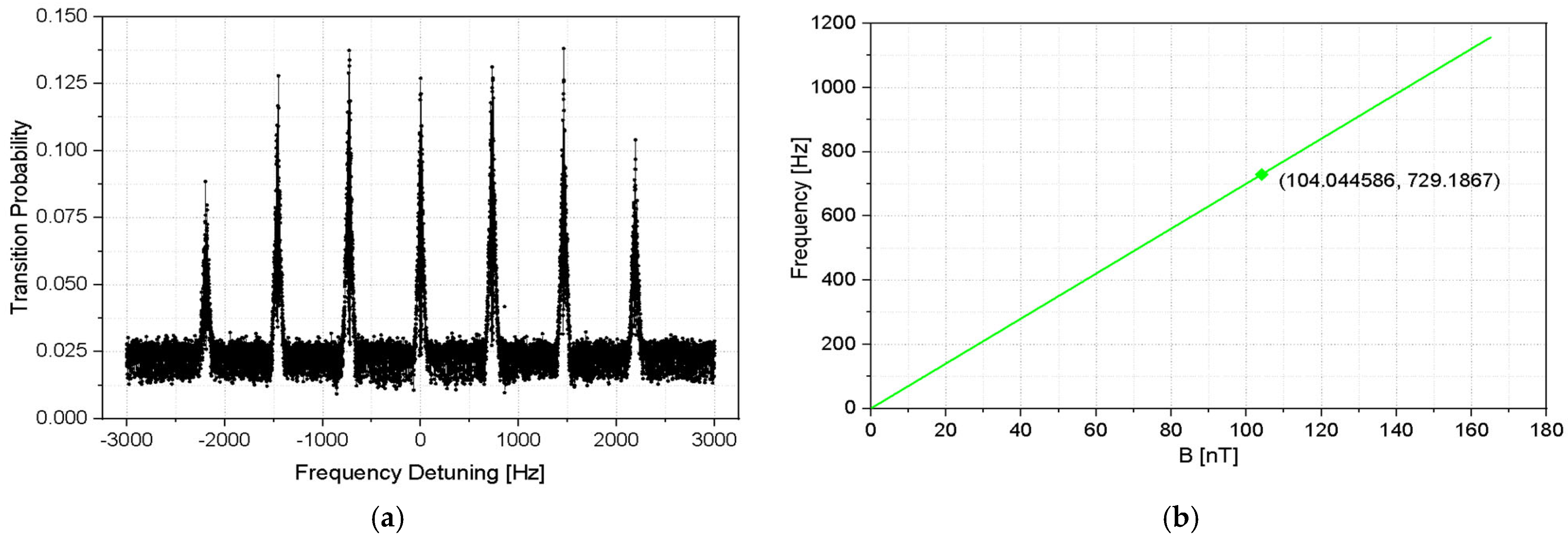
Since the central Ramsey fringe at microwave frequency 9.192631770 GHz is independent of the effect of the magnetic field. The position of m
f = +1 transition as estimated from
Figure 5a,b is approximately 729 Hz (Zeeman offset) shifted to the right of 9.192631770 GHz.
In order to track the m
f = +1 transition, we tune the DDS of the synthesizer to the center frequency of this transition, which is 7.368959 MHz (instead of 7.368230 MHz for central Ramsey), and observe the Ramsey fringes around this frequency. Due to inhomogeneity in the magnetic field B, the central Ramsey fringe shifts relative to the underlying Rabi envelope. This occurs because variations in B induce differential Zeeman shifts across the atomic ensemble, altering the resonance condition for different atoms. As a result, the Ramsey fringes are displaced with respect to the broader Rabi envelope, which originates from the finite duration of the microwave pulse. The Rabi envelope represents the overall spectral response, while the Ramsey fringes provide higher resolution due to the interference between two short π/2 pulses separated by a free evolution time. Since this shift cannot be determined directly, the position of the
central Ramsey fringe was identified by tracking it at different atomic cloud launch heights, with 1 cm increments. The apogee height from the centre of the MOT increases from 53.5 cm to 85.4 cm (
Figure 6). It is easy to identify the center fringe when the atoms are launched just to the center of the Ramsey cavity. The shift in the center fringe is measured for different launch heights, with a 1 cm gap between successive measurements.
To determine the position of the central fringe, we first need to identify the actual central fringe. This is done by processing the data using 5-point averaging and counting the number of fringes from its pedestal. By monitoring the position of the central fringe with changing launch heights of the atoms, a map of
as a function of launch height is obtained. Once the central Ramsey fringe is identified, we find the corresponding
x-axis value. After obtaining the correct
x-axis value, we add 729 MHz, as the Zeeman offset—calculated using the Breit–Rabi formula based on our system’s specifications. This gives us the Zeeman offset value for a specific launch height. We repeat our experiment with different launch heights and calculate the Zeeman offset value. The experimental result is shown in
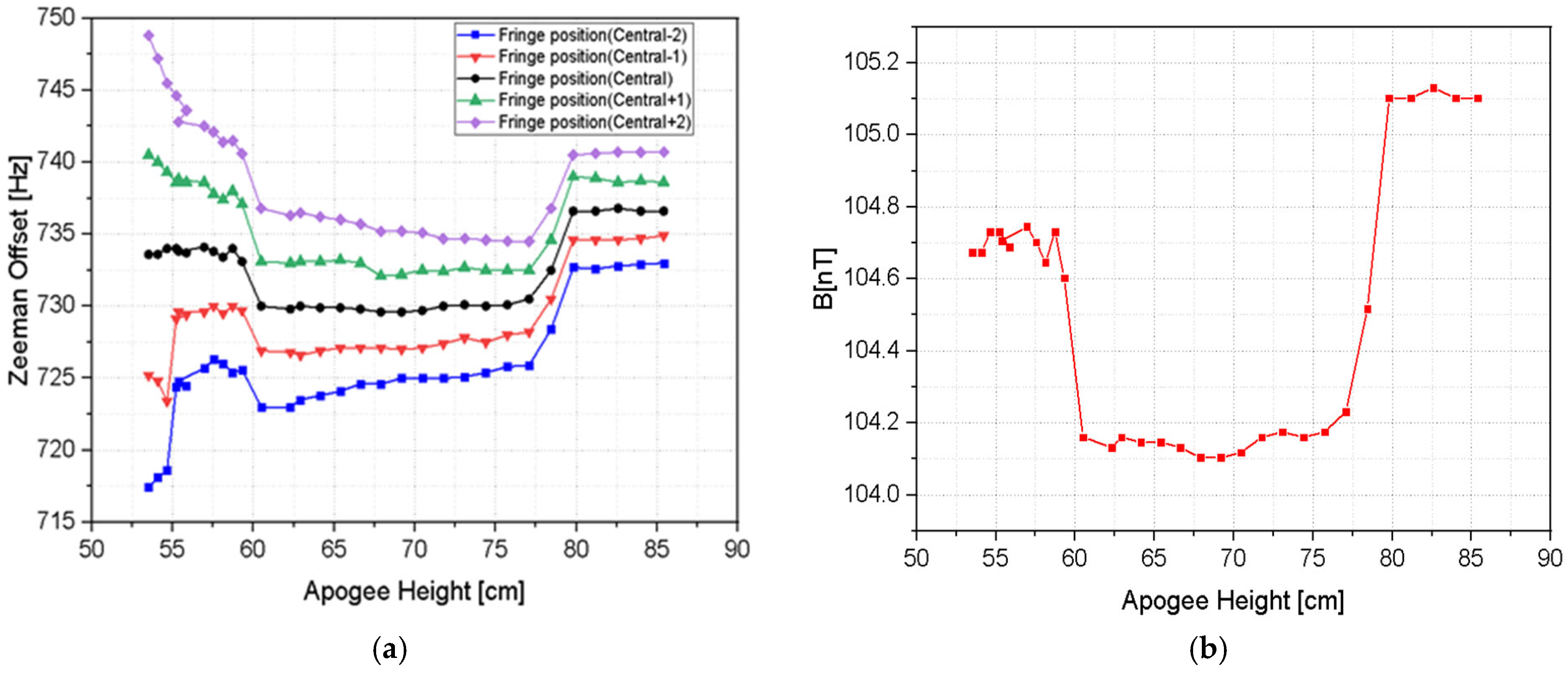
Figure 7a. With the data in
Figure 7a, we use the Breit–Rabi formula to calculate average value of magnetic field at various launch heights. The time-averaged magnetic field ⟨B⟩ is then calculated using the Breit–Rabi formula, and the magnetic field profile is reconstructed by deconvolution of fringe-shift with the ballistic time of flight (
Figure 7b). The magnetic field measured by a magnetometer before the system was vacuum sealed and the one calculated by using cold atoms as quantum sensing probes show similar pattern.
The uncertainty was measured from two components: inhomogeneity and temporal instability in the magnetic field. The inhomogeneity is the standard deviation
of the magnetic field and the uncertainity corresponding to it is given by the following:
From our data,
is 0.13348 nT
2 and contribution to uncertainty due to homogeneity is of the order of 10
−19, which is negligible. The dominant uncertainty is due to the temporal instability and is given by the following:
where
is the temporal variation of
. The position of the central fringe of the magnetically sensitive transition, that is, the m
f = +1 transition, is measured before and after completing the entire set of measurements and a maximum temporal variation of 0.9 Hz is observed. Based on our data,
is 732.44581 Hz and the typical value of
is 9192631770 Hz. This corresponds to an uncertainty of the second order Zeeman shift of the order of 1.24 × 10
−16.
Further, the sensitivity of the magnetic field measurement refers to the minimum detectable change in the magnetic field B. It quantifies how small a change in B can be reliably detected, given the uncertainty in the measurement. It is determined by the second-order Zeeman shift, which arises due to the quadratic dependence of the atomic energy levels on the magnetic field
B. The second-order Zeeman shift Δ
ν2nd is given by the following [
19,
22]:
where
β is the second-order Zeeman coefficient, a parameter that quantifies the strength of the quadratic dependence. The uncertainty in the magnetic field
δ(
B) is related to the fractional uncertainty in the second-order Zeeman shift (
δ(Δ
ν2nd/
ν0)), where
ν0 is the clock transition frequency. Initially, the uncertainty in B can be expressed as follows:
Substituting
B into Equation (10), we obtain the final sensitivity formula:
Thus, the sensitivity of the magnetic field measurement depends on the fractional uncertainty in the second-order Zeeman shift and the second-order Zeeman coefficient β, which is given by 427.45 H z/T2. The sensitivity of the cesium cold atom magnetic sensing is thus calculated as approximately 550 pT/√Hz.
Magnetometers exhibit a wide range of sensitivities depending on their working principles. Our system achieved a sensitivity of approximately 550 pT/√Hz, which places it among the highly sensitive cold atom-based magnetometers. Fluxgate magnetometers typically achieve sensitivities in the 100 pT–1nT/√Hz range [
1], making them suitable for low-frequency applications. Superconducting quantum interference device (SQUID) magnetometers can reach sensitivities of 0.1 pT or even lower [
6], but they require cryogenic cooling. Optically pumped magnetometers, including alkali-vapor magnetometers, offer sensitivities in the range of 1–10 pT/√Hz [
5,
7]. Spin-exchange relaxation-free (SERF) magnetometers operate in near-zero magnetic fields and achieve the highest sensitivities, reaching sub-femtotesla levels [
9]. Chip-scale atomic magnetometers provide compactness with sensitivities around 1–100 pT/√Hz [
8]. Bose–Einstein condensate (BEC)-based magnetometers can reach high resolution with sensitivities in the range of 1 pT/√Hz [
12]. Proton precession magnetometers operate with a sensitivity around 50 nT, mainly used in geophysical surveys [
4]. Our system, with a sensitivity of 550 pT/√Hz, falls within the range of optically pumped and chip-scale atomic magnetometers, making it a competitive choice for precision magnetometry applications.


