Abstract
Sub-Doppler laser-cooled cesium-133 atoms are utilized as quantum sensors to achieve precise mapping of magnetic fields across a region in ultra-high vacuum (UHV), with a spatial resolution of 1 cm and a sensitivity of approximately 550 pT/√Hz, enabling accurate measurements within the nanotesla [nT] range. The cold cesium-133 atoms used for magnetic field measurements in this paper are a key component of the cesium fountain frequency standard at CSIR-NPL, which contributes to both timekeeping and magnetic sensing. The results show magnetic field fluctuations within 1 nT with a spatial resolution of 1 cm. The uncertainty in these measurements is of the order of 1.24 × 10⁻¹⁶, ensuring reliable and precise spatially resolved magnetic field mapping.
1. Introduction
Magnetic field sensing is crucial for understanding many concepts of fundamental and applied sciences, with different applications in the fields of quantum metrology, space research, and navigation, among others. Conventional magnetic sensors such as fluxgate magnetometers [1] and Hall-effect sensors utilize classical electromagnetic coupling between the field and the probe. These devices offer a detection range from 1 nT to 107 nT and a sensitivity limited to 1 nT/√Hz. In contrast, quantum magnetic sensors such as the SQUIDs [2] (Superconducting Quantum Interference Device), provide much higher sensitivities for measuring weak magnetic fields, with sensitivities around 1 fT/√Hz. However, they are constrained by the need for complex and costly cryogenic systems and limited spatial resolution [3,4,5,6].
In the past 20 years, atomic magnetic sensing methods [7,8] based on neutral atoms have emerged as a compact, non-cryogenic alternative for achieving sub-femtotesla sensitivity in weak magnetic fields. Thermal atomic magnetic sensing techniques operate at room temperature and use atomic vapors to measure magnetic fields, achieving sensitivities down to about 1 fT/√Hz. However, they are limited by thermal noise and Doppler broadening due to high atomic velocities, affecting their precision and spatial resolution [3,9,10].
Cold or ultra-cold systems [11] improve on this by using cold atomic ensembles or Bose–Einstein condensates (BECs) [12,13,14], which have significantly reduced thermal velocities. This reduction minimizes thermal noise and sharpens resonance signals, resulting in much higher sensitivities, often reaching the sub-femtotesla range, and higher spatial resolution. Their ability to manipulate quantum states and maintain longer coherence times makes cold atomic magnetometers superior for precise magnetic field measurements. However, these experiments involve sophisticated setups and detailed protocols and depend upon imaging of the atomic cloud. Additionally, the achieved sensitivities often fall short of those provided by thermal atomic magnetic sensing methods, and the magnetic field is measured indirectly. Consequently, the practical application of cold atomic magnetic sensing techniques remained limited [3,14,15,16].
In this paper, we demonstrate and characterize quantum sensing measurements to observe spatially resolved magnetic field variations using cesium-133 atoms cooled to approximately 3 µK. The cesium fountain atomic clock measures the clock transition frequency of 9,192,631,770 Hz with high precision [17,18,19]. To ensure accurate measurements of this frequency, the degeneracy of the hyperfine state must be removed. Thus, after laser cooling, a hyperfine state sensitive to the magnetic field is created through a uniform magnetic field produced by a solenoid, enabling precise mapping of magnetic field variations. The cold cesium atoms are launched using frequency detuned vertical laser beams. During their ballistic flight, the atoms interact with the microwaves, reach a height, and then fall back under gravity. As they exit the flight tube, two horizontal detection beams are turned on, and the fluorescence signal is collected by large-area photodiodes and is monitored on a PC via a data acquisition (DAQ) card. The Ramsey method of interrogation is employed to achieve high-resolution atomic transition frequency measurements with reduced Doppler broadening and high sensitivity to phase differences. The Direct digital synthesizer (DDS) frequency is scanned to produce Ramsey fringes for precise atomic transition frequency measurements. Ramsey fringes for magnetic field sensitive states are observed at various launch heights of the atomic cloud. The central fringe frequency varies with launch height, allowing the creation of a map of the magnetic field as a function of height by deconvoluting the fringe shift data. Hence, we trace the magnetic field within the ultrahigh vacuum using cesium atoms as quantum magnetic sensors, providing spatially resolved measurements of magnetic field variations across the experimental region. In a shielded environment, we achieve a magnetic field sensitivity of approximately 550 pT/√Hz.
2. Experimental Setup
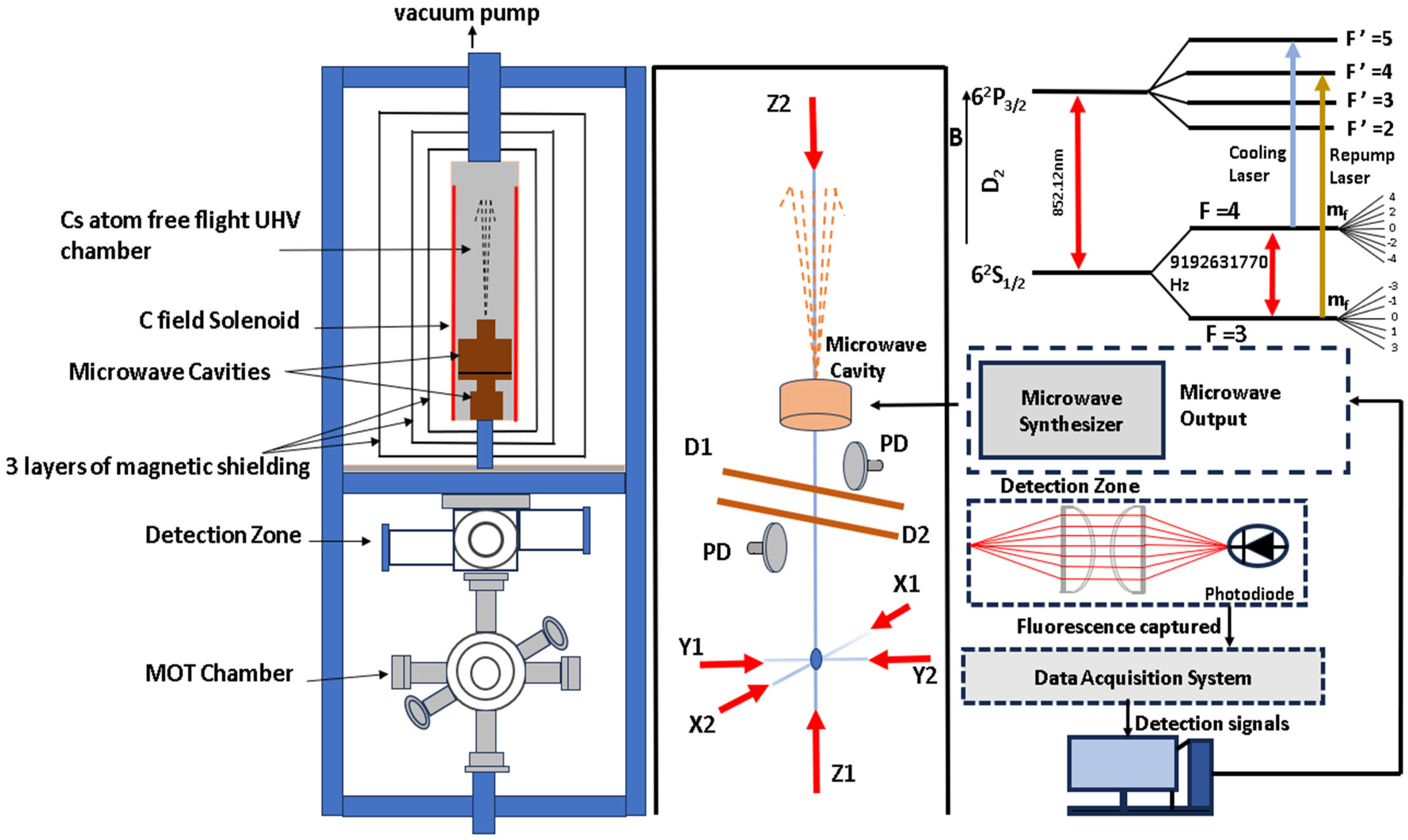
The system, as shown in Figure 1, features a magneto-optical trap (MOT) with a (0, 0, 1) geometry, aligned along the Z-axis, for cooling and launching the cesium atoms. The cesium atoms are cooled in a 3D MOT and then further cooled in optical molasses (OM) inside an octagonal stainless-steel chamber. A quadrupole magnetic field gradient of 6 G/cm is produced in the trapping region by two coils, each with a radius of 75 mm and 100 turns in an anti-Helmholtz configuration. Furthermore, the background magnetic field at the atoms’ location is compensated for by three pairs of Helmholtz coils (pointing in the X, Y, and Z directions) surrounding the MOT. A temperature-controlled cold finger with a Cs ampoule connected to the MOT chamber is the source of Cs [18,20].
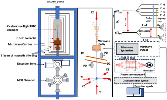
Figure 1.
Schematic of the NPLI– CsF1 cesium fountain atomic clock setup for cold atom magnetic sensing. The C–field (magnetic field B produced by solenoid as shown in the figure) is generated by a solenoid and measured using laser-cooled cesium atoms. X1, X2, Y1, Y2, Z1, and Z2 are six cooling beams arranged in a (0, 0, 1) geometry along the Z direction. D1 and D2 are detection beams, with a photodiode (PD) positioned orthogonally to capture fluorescence. The detection chamber includes a lens system for efficient fluorescence collection.
The cooling process includes an Extended cavity diode laser (ECDL at 852 nm) in Littrow mode which is frequency locked to a cesium D2 line [crossover peak of 133Cs 6 2S1/2 (F = 4) → 6 2P3/2 (F′ = 4 and 5)], generated by high-resolution saturated absorption spectroscopy. The laser output is amplified by a tapered amplifier system (Toptica TA Pro) and is divided into four horizontal cooling beams with an average intensity of 10 mW cm−2 per MOT beam and two vertical beams with an average intensity of 3 mW cm−2 per beam. Besides the cooling beams, the optical setup provides two beams for detection (D1, D2) with average intensity of 2 mW cm−2 per beam. A re-pumping laser (ECDL at 852 nm) is tuned and locked to the transition 133Cs 6 2S1/2 (F = 3, mf = 0) → 6 2P3/2 (F′ = 4, mf = 0) by high-precision laser saturated absorption spectroscopy. The output beam is split and mixed with one of the cooling beams, Y2, and a detection beam, D2, with average intensity of 5 mW cm−2. Acousto-optic modulators (AOMs) in a double-pass configuration are used to regulate the frequency and intensity of the cooling beams. Quick switching between lasers is achieved using mechanical shutters and computer-controlled AOMs. The mechanical shutters feature a rise time of approximately 500 µs and a fall time of approximately 400 µs, enabling efficient and precise control over the laser beams.
The atomic trap is monitored via destructive absorption imaging and real-time fluorescence imaging. Directly above the MOT is the detection chamber, and above it is the aluminium flight tube, enclosed within three layers of mu metal magnetic shield. Two horizontal, parallel detection beams are spaced 45 mm vertically apart and are individually formed into 10 mm squares using apertures. The fluorescence collector ensembles for the atoms in the two states F = 4 and F = 3 are positioned perpendicular to the detection laser beams. Each ensemble comprises of a pair of achromatic plano-convex imaging lenses (50 mm diameter and 75 mm focal length), as shown in Figure 1, arranged back-to-back, focusing the light onto a large-area silicon photodiode (10 mm square) [18,20].
Within the flight tube, there are two microwave cavities: the Ramsey cavity and the state-selection cavity. The center of the Ramsey cavity is located 52.5 cm above the trap center. The source for the microwave interrogation is a synthesizer that has been designed in collaboration with PTB, Germany. A uniform C-field which lifts the degeneracy of the energy states and splits them into 2F + 1 Zeeman levels for accurate measurement of the clock transition frequency is produced using a solenoid with 320 turns wound on a former with a diameter of 235 mm and length of 640 mm, ensuring a stable magnetic environment and minimizing uncertainties in frequency evaluation. The C-field generates a magnetic field of 104 nT. The solenoid is placed inside the innermost mu metal shield and, together with three additional compensation coils at the top and bottom, produces a homogeneous C-field of about 104 nT over the drift region. Two 55 l/s ion pumps on the top of the vacuum assembly keep the pressure inside the flight tube at 8 × 10⁻⁸ Pa [18].
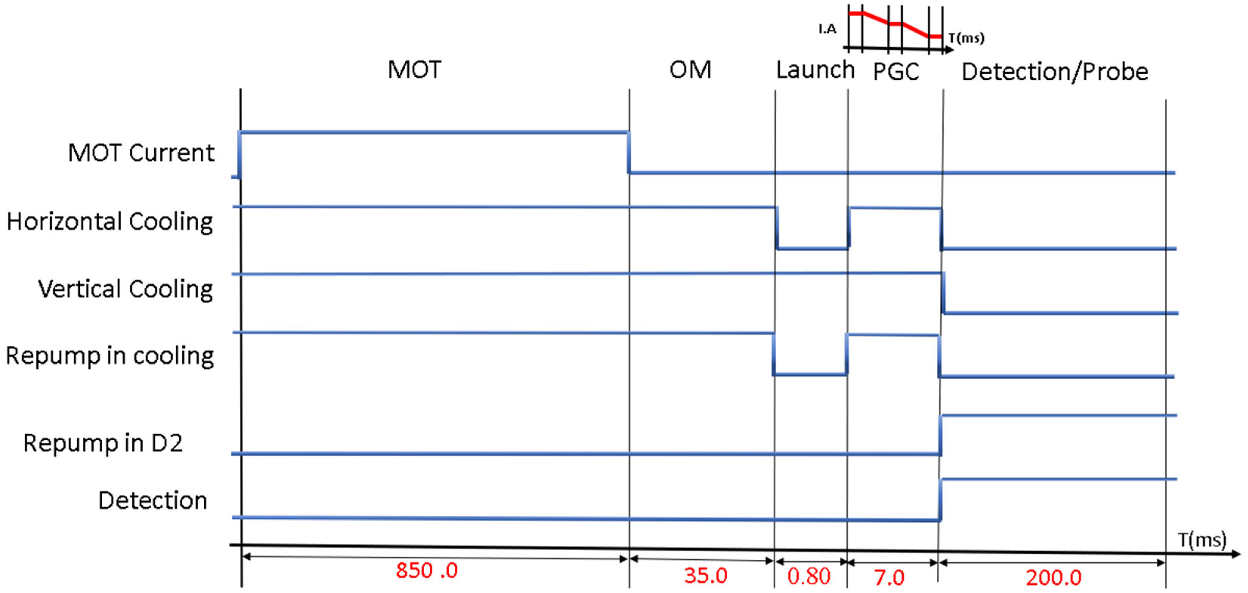
The timing sequence generation [18,20] proceeds as sketched in Figure 2 to run the process from MOT loading to polarization gradient cooling and measurement of detection signal. Initially, the cooling laser is frequency detuned by approximately −2Γ, where Γ = 5.2 MHz [21], and atoms are typically loaded for up to 850 ms in the MOT. The atomic cloud is then further cooled by optical molasses for 35 ms. The atoms are then launched using moving molasses and cooled further with Polarization gradient cooling (PGC) for 7 ms, which brings the atoms’ temperature down to approximately 3 µk. Up to 107 atoms are trapped in the PGC phase. During this phase, the intensity of the cooling beams is gradually reduced while the detuning is incrementally increased, achieved through a frequency ramp as shown in Figure 2. After cooling, all laser beams are turned off, and the atoms are launched by applying frequency-detuned vertical laser beams, with the upward directed beam tuned to a frequency and the downward beam tuned to a frequency , imparting an initial velocity that causes the atoms to ascend to a height Hm and then fall back under gravity.

Figure 2.
The figure illustrates the timing sequence of different laser and magnetic field pulses during various experimental phases. The pulse signals indicate the on/off states of different processes, while T(ms) is optimized by considering various experimental parameters. The red graph represents the frequency ramp of laser intensity amplitude (I.A) during the PGC phase as a function of time (in ms).
During this ballistic flight, the atoms interact with two microwave (π/2) pulses in the Ramsey interrogation process. The first pulse excites the cesium atoms from the ground state into a superposition of the F = 3 and F = 4 states. After a delay, the second pulse allows the atoms to interact with the microwave field again, leading to an interference pattern known as Ramsey fringes. Thus, the atomic cloud interacts with the Ramsey cavity twice, and the time interval between these pulses determines the coherence and phase of the superposition, producing the observed Ramsey fringe pattern. As the atoms exit the flight tube, detection beams are turned on. Photodiodes capture the fluorescence signal from the falling atoms within a detection window of 200 ms and transmit it to the PC through a data acquisition (DAQ) card. Microcontroller-based cards regulate the entire timing sequence, and a LabVIEW application handles data processing and acquisition.
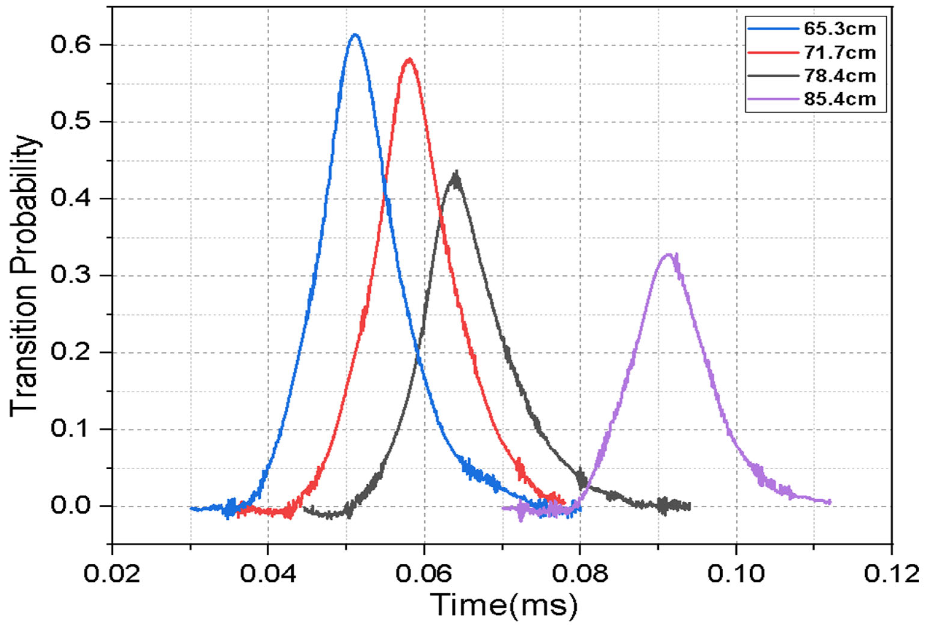
Atoms can be launched to various heights by changing the launch frequency, and the time of arrival (time between the launch and when the atomic cloud) is detected. Higher launch velocities lead to greater heights and longer time of arrival. As launch height increases, the atomic cloud expands more, resulting in greater atom loss when passing through the microwave cavities. A cooler and more tightly confined cesium cloud can be launched higher with less expansion. Figure 3 shows the return signals with increasing launch velocities and thus increasing launch heights and times of arrivals.
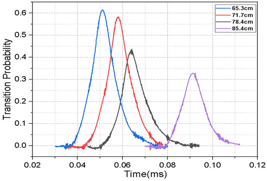
Figure 3.
Relative atomic fluorescence as a function of time for various toss heights. As the toss height increases, fewer atoms return to the detection zone, resulting in a decreased fluorescence signal. The signal reflects the detection of cold cesium atoms at varying heights during their ballistic motion.
3. Results and Discussion
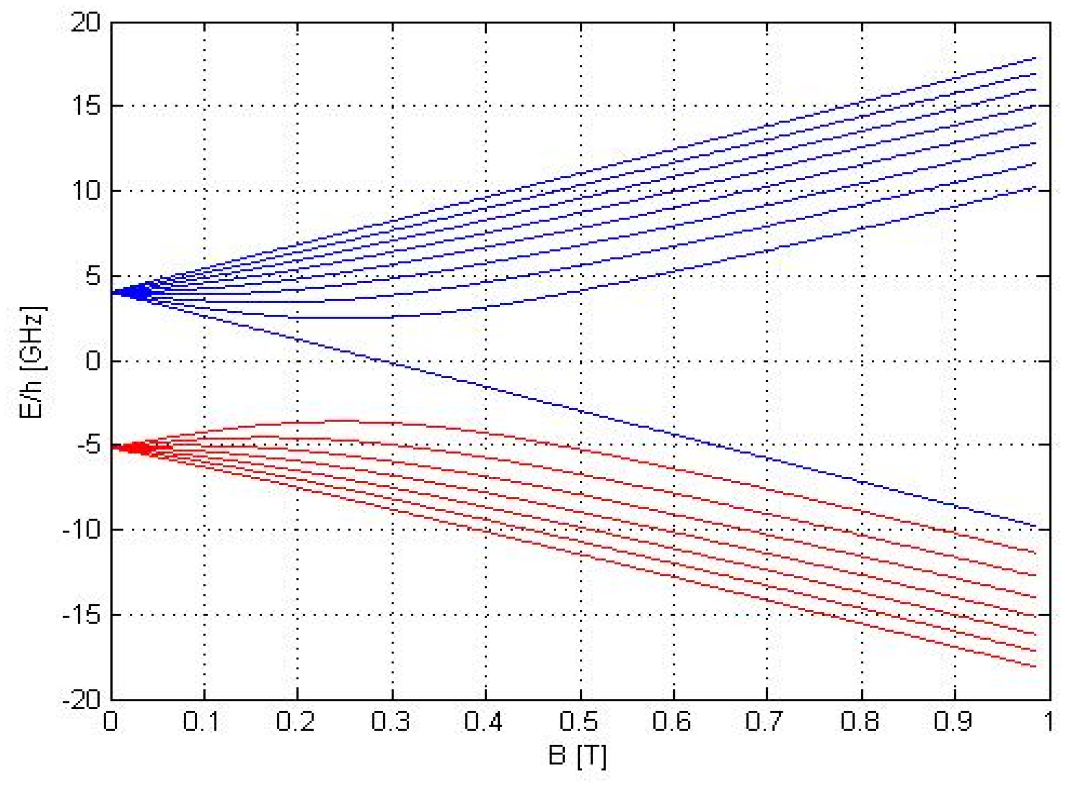
To precisely measure the magnetic field strength inside the flight tube, we utilize the linear Zeeman frequency shift of magnetically sensitive transitions since, the clock transition is not very sensitive to the magnetic field changes and has a small frequency shift proportional to . In general, Zeeman shift is measured by measuring the shift in the central fringe for the transition which has a linear dependence on the magnetic field B. If we denote the difference between the transition and the transition as and neglect higher orders, the 2nd order Zeeman shift is given by the Breit–Rabi formula (solution given in Figure 4) as follows [19,22]:
where = 2.00254032 and = −0.00039885395 are Lande -factors of the electron and the nucleus, µB = 9.27400899 × 10⁻²⁴ J. T−1 is the Bohr magnetron [21], ν0 is the clock transition frequency , brackets ⟨ ⟩ indicate a time-averaged value over the interaction time T, and is the mean squared magnetic field averaged over the flight region above the microwave cavity. When the C-field is inhomogeneous, is given by the following:
where is the variance of B along the atomic trajectory.
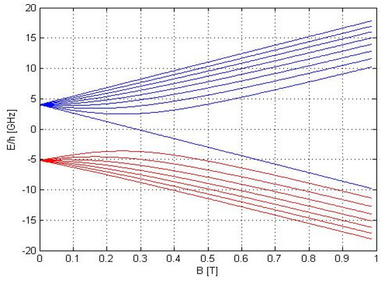
Figure 4.
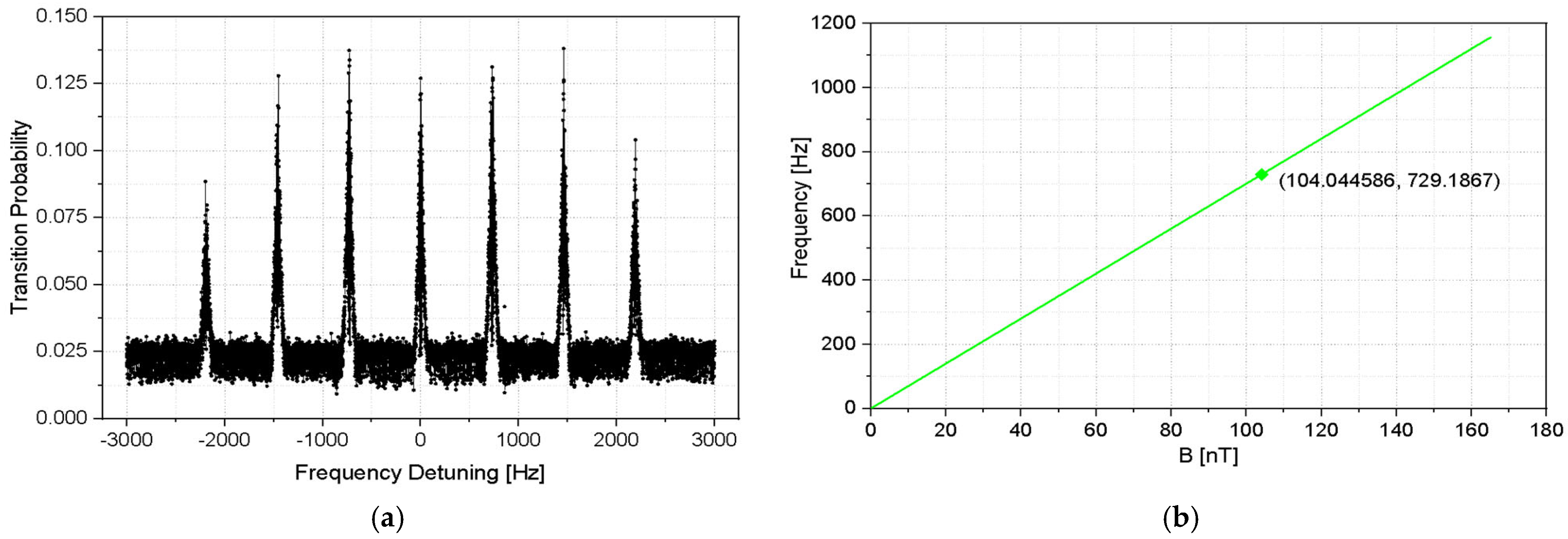
Solution of the Breit–Rabi formula. The plot shows frequency shift vs. magnetic field as derived from the Breit–Rabi formula. The blue curves represent the frequency shifts for the F = 4, mf levels, while the red curves correspond to the F = 3, mf levels. The nonlinear Zeeman effect is evident as the energy levels deviate from a linear dependence at higher magnetic fields. To measure the magnetic field inside the ultra-high vacuum, a long Ramsey scan is performed to identify the exact positions of the mf = ±1, ±2, and ±3 states. This involves scanning the frequency of the microwave synthesizer from −3000 Hz to +3000 Hz to locate the position of the central fringe of the transition (as shown in Figure 5a). The microwave frequency synthesizer precisely controls the microwave signal used for Ramsey interrogation of the atoms. It enables accurate frequency generation and allows for controlled frequency detuning, which is crucial for measuring the atomic resonance. The position is confirmed theoretically from the solution of the Breit–Rabi formula (Equation (2)) for mf = 1 transition (with a known value of B = 104 nT), as shown in Figure 5b.
Using Equations (1)–(4), the second-order Zeeman shift is given by the following:
Further, the uncertainty of the 2nd order Zeeman shift is given by the temporal instability of :
where is the temporal variation of .
Since the central Ramsey fringe at microwave frequency 9.192631770 GHz is independent of the effect of the magnetic field. The position of mf = +1 transition as estimated from Figure 5a,b is approximately 729 Hz (Zeeman offset) shifted to the right of 9.192631770 GHz.
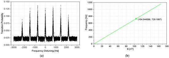
Figure 5.
(a) The figure shows a long Ramsey scan for mf = ±1, ±2, and ±3 states. This gives the experimental determination of the mf = +1 transition position. The observed fringe patterns correspond to the atomic coherence time and help identify the precise resonance position. (b) This figure shows the Zeeman shift as a function of magnetic field for mf = +1 transition, which gives theoretical confirmation of the mf = +1 transition position. The linear dependence validates the expected shift behavior under varying field strengths.
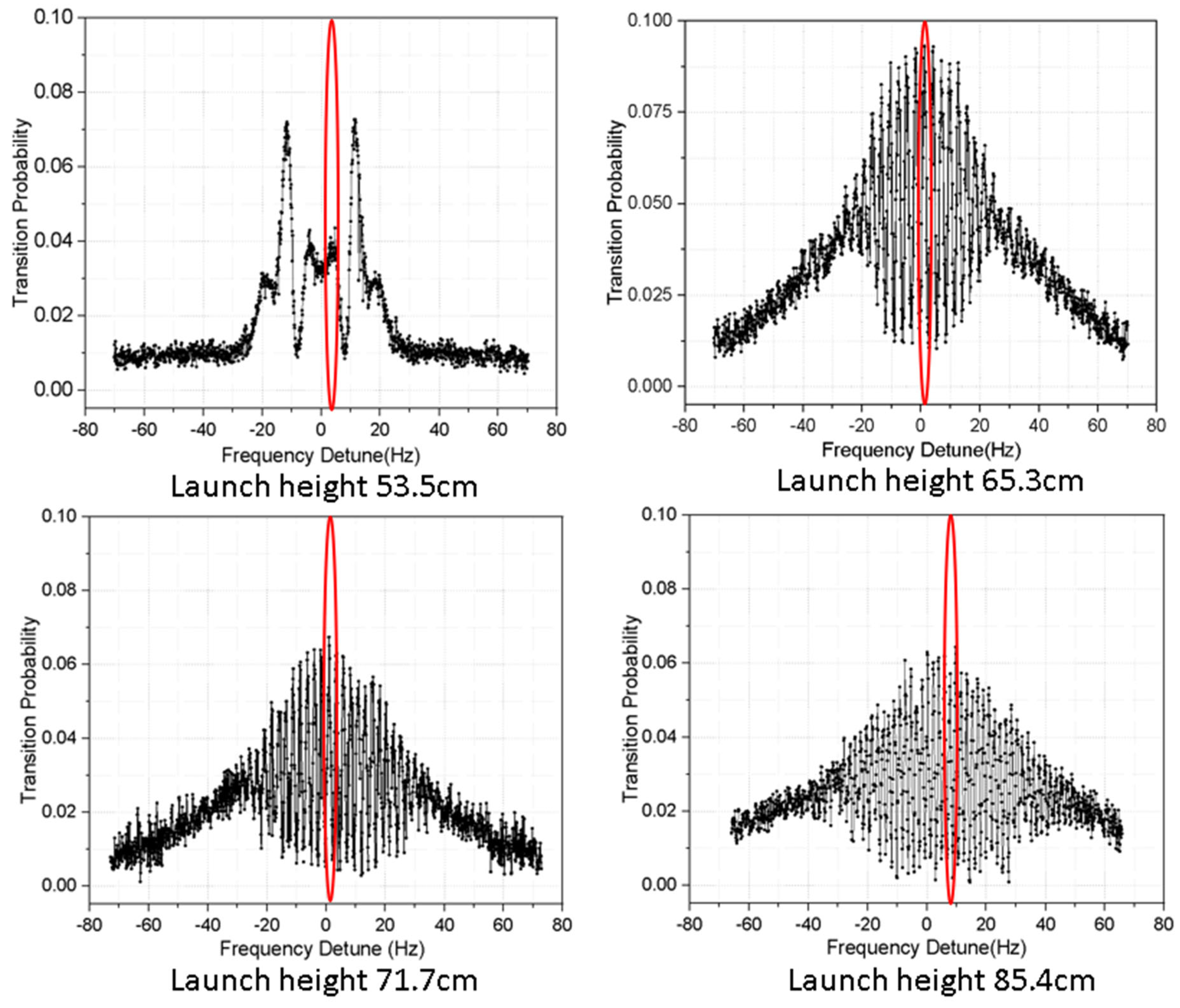
In order to track the mf = +1 transition, we tune the DDS of the synthesizer to the center frequency of this transition, which is 7.368959 MHz (instead of 7.368230 MHz for central Ramsey), and observe the Ramsey fringes around this frequency. Due to inhomogeneity in the magnetic field B, the central Ramsey fringe shifts relative to the underlying Rabi envelope. This occurs because variations in B induce differential Zeeman shifts across the atomic ensemble, altering the resonance condition for different atoms. As a result, the Ramsey fringes are displaced with respect to the broader Rabi envelope, which originates from the finite duration of the microwave pulse. The Rabi envelope represents the overall spectral response, while the Ramsey fringes provide higher resolution due to the interference between two short π/2 pulses separated by a free evolution time. Since this shift cannot be determined directly, the position of the central Ramsey fringe was identified by tracking it at different atomic cloud launch heights, with 1 cm increments. The apogee height from the centre of the MOT increases from 53.5 cm to 85.4 cm (Figure 6). It is easy to identify the center fringe when the atoms are launched just to the center of the Ramsey cavity. The shift in the center fringe is measured for different launch heights, with a 1 cm gap between successive measurements.
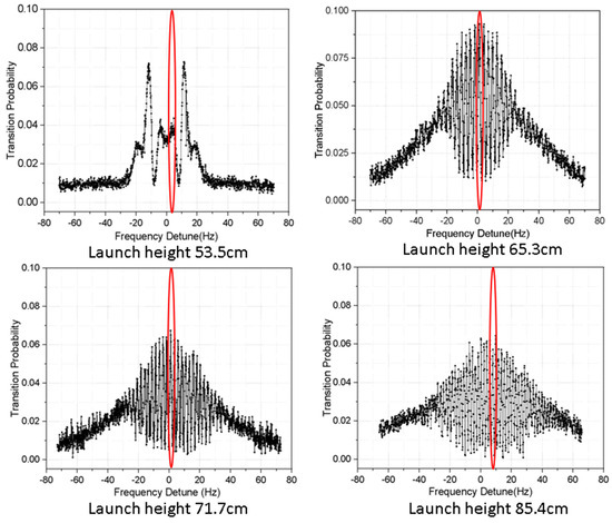
Figure 6.
The Ramsey fringes of the magnetic field sensitive transition at different launch heights in the NPLI-CsF1 cesium fountain clock. The fringe shift is calculated at different positions with 1 cm gap from 53.5 cm to 85.4 cm, with four representative patterns shown in the figure. Red ellipses highlight the position of the central fringe to clearly illustrate the fringe shift with varying launch height.
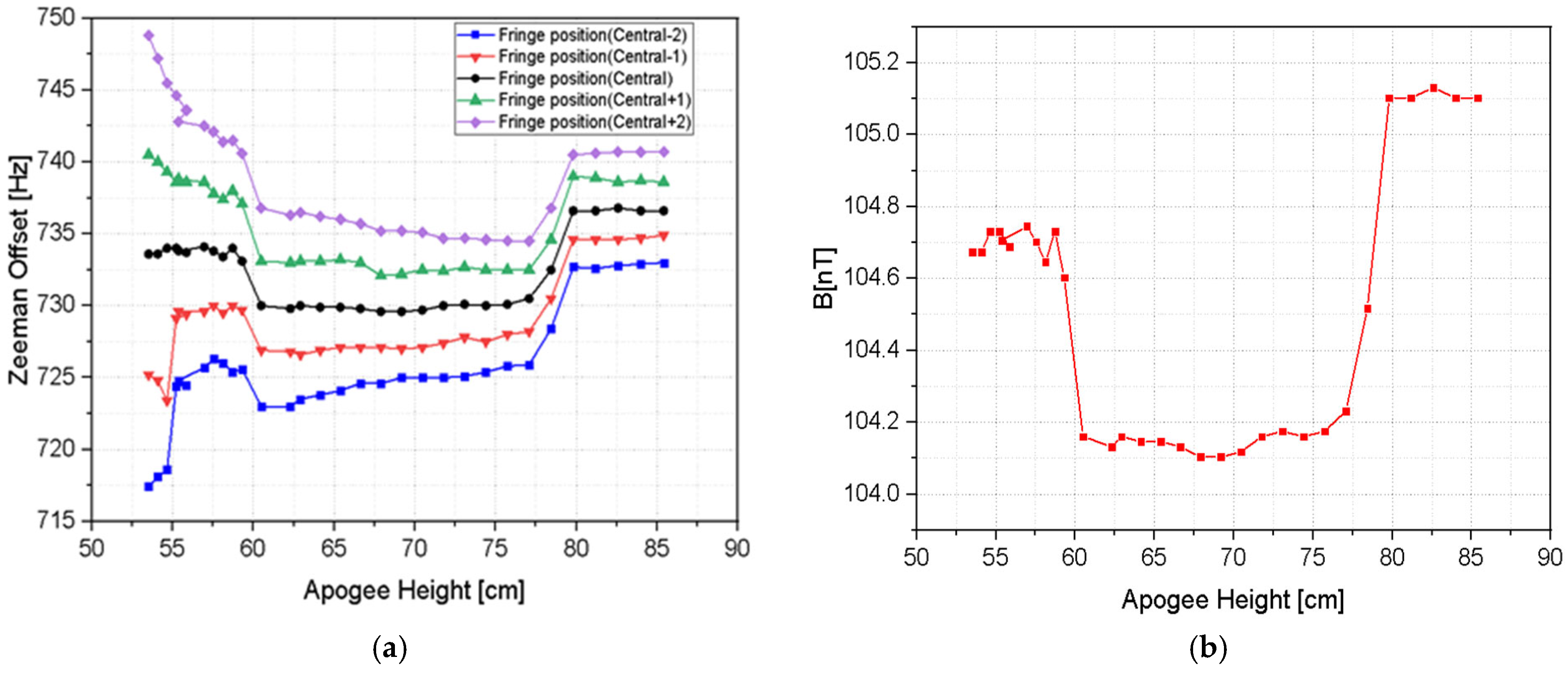
To determine the position of the central fringe, we first need to identify the actual central fringe. This is done by processing the data using 5-point averaging and counting the number of fringes from its pedestal. By monitoring the position of the central fringe with changing launch heights of the atoms, a map of as a function of launch height is obtained. Once the central Ramsey fringe is identified, we find the corresponding x-axis value. After obtaining the correct x-axis value, we add 729 MHz, as the Zeeman offset—calculated using the Breit–Rabi formula based on our system’s specifications. This gives us the Zeeman offset value for a specific launch height. We repeat our experiment with different launch heights and calculate the Zeeman offset value. The experimental result is shown in Figure 7a. With the data in Figure 7a, we use the Breit–Rabi formula to calculate average value of magnetic field at various launch heights. The time-averaged magnetic field ⟨B⟩ is then calculated using the Breit–Rabi formula, and the magnetic field profile is reconstructed by deconvolution of fringe-shift with the ballistic time of flight (Figure 7b). The magnetic field measured by a magnetometer before the system was vacuum sealed and the one calculated by using cold atoms as quantum sensing probes show similar pattern.
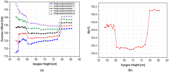
Figure 7.
(a) Zeeman offset as a function of launch height observed for the central fringe and two neighbouring fringes on either side. The variation in offset arises due to inhomogeneity in the magnetic field throughout the flight tube and is analyzed as a function of launch heights. (b) The magnetic field is obtained by deconvoluting the Zeeman offset using the Breit–Rabi formula and is then given as a function of height, showing the field distribution experienced by the cold atoms during their ballistic trajectory through the solenoidal C-field. The measured field variation helps characterize the spatial magnetic field profile within the region.
The uncertainty was measured from two components: inhomogeneity and temporal instability in the magnetic field. The inhomogeneity is the standard deviation of the magnetic field and the uncertainity corresponding to it is given by the following:
From our data, is 0.13348 nT2 and contribution to uncertainty due to homogeneity is of the order of 10−19, which is negligible. The dominant uncertainty is due to the temporal instability and is given by the following:
where is the temporal variation of . The position of the central fringe of the magnetically sensitive transition, that is, the mf = +1 transition, is measured before and after completing the entire set of measurements and a maximum temporal variation of 0.9 Hz is observed. Based on our data, is 732.44581 Hz and the typical value of is 9192631770 Hz. This corresponds to an uncertainty of the second order Zeeman shift of the order of 1.24 × 10⁻¹⁶.
Further, the sensitivity of the magnetic field measurement refers to the minimum detectable change in the magnetic field B. It quantifies how small a change in B can be reliably detected, given the uncertainty in the measurement. It is determined by the second-order Zeeman shift, which arises due to the quadratic dependence of the atomic energy levels on the magnetic field B. The second-order Zeeman shift Δν2nd is given by the following [19,22]:
where β is the second-order Zeeman coefficient, a parameter that quantifies the strength of the quadratic dependence. The uncertainty in the magnetic field δ(B) is related to the fractional uncertainty in the second-order Zeeman shift (δ(Δν2nd/ν0)), where ν0 is the clock transition frequency. Initially, the uncertainty in B can be expressed as follows:
Substituting B into Equation (10), we obtain the final sensitivity formula:
Thus, the sensitivity of the magnetic field measurement depends on the fractional uncertainty in the second-order Zeeman shift and the second-order Zeeman coefficient β, which is given by 427.45 H z/T2. The sensitivity of the cesium cold atom magnetic sensing is thus calculated as approximately 550 pT/√Hz.
Magnetometers exhibit a wide range of sensitivities depending on their working principles. Our system achieved a sensitivity of approximately 550 pT/√Hz, which places it among the highly sensitive cold atom-based magnetometers. Fluxgate magnetometers typically achieve sensitivities in the 100 pT–1nT/√Hz range [1], making them suitable for low-frequency applications. Superconducting quantum interference device (SQUID) magnetometers can reach sensitivities of 0.1 pT or even lower [6], but they require cryogenic cooling. Optically pumped magnetometers, including alkali-vapor magnetometers, offer sensitivities in the range of 1–10 pT/√Hz [5,7]. Spin-exchange relaxation-free (SERF) magnetometers operate in near-zero magnetic fields and achieve the highest sensitivities, reaching sub-femtotesla levels [9]. Chip-scale atomic magnetometers provide compactness with sensitivities around 1–100 pT/√Hz [8]. Bose–Einstein condensate (BEC)-based magnetometers can reach high resolution with sensitivities in the range of 1 pT/√Hz [12]. Proton precession magnetometers operate with a sensitivity around 50 nT, mainly used in geophysical surveys [4]. Our system, with a sensitivity of 550 pT/√Hz, falls within the range of optically pumped and chip-scale atomic magnetometers, making it a competitive choice for precision magnetometry applications.
4. Conclusions
We have demonstrated a cold atom magnetic sensing technique using polarization gradient cooling (PGC) of cesium-133, achieving a sensitivity of approximately 550 pT/√Hz. This proof-of-concept system highlights the potential of spatially resolved magnetic field measurements, leveraging the high control and precision inherent in cold atom systems. The successful implementation of this approach paves the way for advancements in quantum sensing [16], where atomic magnetometers (AMs) can be integrated with enhanced spatial resolution and control. The results show magnetic field fluctuations within 1 nT with a spatial resolution of 1 cm. The uncertainty in these measurements is of the order of 1.24 × 10⁻¹⁶, ensuring reliable and precise spatially resolved magnetic field mapping and offering new opportunities for highly sensitive, spatially resolved measurements of magnetic fields. Moreover, this system holds potential for miniaturization in the future, focusing on magnetic sensing measurements with reduced size and improved portability. The measurement relies on detecting the Zeeman shift due to magnetic field inhomogeneity, which remains unchanged regardless of system size. Future miniaturization efforts could leverage advanced techniques such as miniature laser cooling setups, compact vacuum chambers, and optimized optical configurations. These modifications would enable precise magnetic field measurements over a corresponding region while significantly reducing the overall physical footprint of the system. Importantly, the core measurement principles—including the detection of the Zeeman shift as an indicator of magnetic field variations—would remain unchanged.
Author Contributions
Conceptualization, P.A. and M.D.; methodology and calculation, A.B.; validation, M.D. and P.A.; data curation, A.B.; writing—original draft preparation, A.B.; review and editing, M.D. and P.A.; supervision, M.D. and P.A.; funding acquisition, P.A. All authors have read and agreed to the published version of the manuscript.
Funding
This work is funded by the Council of Scientific and Industrial Research (CSIR) under the project HCP-55. The authors gratefully acknowledge CSIR-NPL. A.B. acknowledges fellowship from UGC. It is only through their invaluable support that this experiment was made possible.
Data Availability Statement
The datasets/database generated during and/or analyzed during the study/research are available from the corresponding author on reasonable request.
Acknowledgments
The authors gratefully acknowledge Amitava Sen Gupta for his valuable insights and scientific discussions.
Conflicts of Interest
The authors of this research article declare that there are no conflicts of interest that could influence the objectivity, impartiality, or integrity of the research findings and their interpretation.
References
- Primdahl, F. The fluxgate magnetometer. J. Phys. E Sci. Instrum. 1979, 12, 4. [Google Scholar] [CrossRef]
- John, C.; Braginski, A.I. The SQUID Handbook: Applications of SQUIDs and SQUID Systems; John Wiley & Sons: Hoboken, NJ, USA, 2006. [Google Scholar]
- Zhang, Q.; Wang, Y.; Zhu, C.; Wang, Y.; Zhang, X.; Gao, K.; Zhang, W. Precision measurements with cold atoms and trapped ions. Chin. Phys. B 2020, 29, 9. [Google Scholar] [CrossRef]
- Ripka, P. Magnetic sensors and magnetometers. Meas. Sci. Technol. 2002, 13, 645. [Google Scholar]
- Budker, D.; Romalis, M. Optical magnetometry. Nat. Phys. 2007, 3, 227–234. [Google Scholar] [CrossRef]
- Fagaly, R.L. Superconducting quantum interference device instruments and applications. Rev. Sci. Instrum. 2006, 77, 101101. [Google Scholar] [CrossRef]
- Kominis, I.K.; Kornack, T.W.; Allred, J.C.; Romalis, M.V. A subfemtotesla multichannel atomic magnetometer. Nature 2003, 422, 596–599. [Google Scholar] [CrossRef] [PubMed]
- Dang, H.B.; Maloof, A.C.; Romalis, M.V. Ultrahigh sensitivity magnetic field and magnetization measurements with an atomic magnetometer. Appl. Phys. Lett. 2010, 97, 151110. [Google Scholar] [CrossRef]
- Schwindt, P.D.D.; Knappe, S.; Shah, V.; Hollberg, L.; Kitching, J.; Liew, L.-A.; Moreland, J. Chip-scale atomic magnetometer. Appl. Phys. Lett. 2004, 85, 6409–6411. [Google Scholar] [CrossRef]
- Shen, H. Spin Squeezing and Entanglement with Room Temperature Atoms for Quantum Sensing and Communication. Ph.D. Thesis, University of Copenhagen, Copenhagen, Denmark, 2014. [Google Scholar]
- Geiger, R.; Landragin, A.; Merlet, S.; Dos Santos, F.P. High-accuracy inertial measurements with cold-atom sensors. AVS Quantum Sci. 2020, 2, 024702. [Google Scholar] [CrossRef]
- Vengalattore, M.; Higbie, J.M.; Leslie, S.R.; Guzman, J.; Sadler, L.E.; Stamper-Kurn, D.M. High-resolution magnetometry with a spinor bose-einstein condensate. Phys. Rev. Lett. 2007, 98, 200801. [Google Scholar] [CrossRef] [PubMed]
- Wildermuth, S.; Hofferberth, S.; Lesanovsky, I.; Groth, S.; Krüger, P.; Schmiedmayer, J.; Bar-Joseph, I. Sensing electric and magnetic fields with Bose-Einstein condensates. Appl. Phys. Lett. 2006, 88, 264103. [Google Scholar] [CrossRef]
- Cohen, Y.; Jadeja, K.; Sula, S.; Venturelli, M.; Deans, C.; Marmugi, L.; Renzoni, F. A cold atom radio-frequency magnetometer. Appl. Phys. Lett. 2019, 114, 073505. [Google Scholar] [CrossRef]
- Koschorreck, M.; Napolitano, M.; Dubost, B.; Mitchell, M.W. High resolution magnetic vector-field imaging with cold atomic ensembles. Appl. Phys. Lett. 2011, 98, 074101. [Google Scholar] [CrossRef]
- Dutta, P.; Maurya, S.S.; Patel, K.; Biswas, K.; Mangaonkar, J.; Sarkar, S.; Rapol, U.D. A Decade of Advancement of Quantum Sensing and Metrology in India Using Cold Atoms and Ions. J. Indian Inst. Sci. 2023, 103, 609–632. [Google Scholar] [CrossRef]
- Wynands, R.; Weyers, S. Atomic fountain clocks. Metrologia 2005, 42, 3. [Google Scholar] [CrossRef]
- Gupta, A.S.; Agarwal, A.; Arora, P.; Pant, K. Development of cesium fountain frequency standard at the National Physical Laboratory, India. Curr. Sci. 2011, 100, 1393–1399. [Google Scholar]
- Vanier, J.; Audoin, C. The Atomic Frequency Standards; Adam Hilger: Bristol, UK, 1989. [Google Scholar]
- Acharya, A.; Bharath, V.; Arora, P.; Yadav, S.; Agarwal, A.; Gupta, A.S. Systematic uncertainty evaluation of the cesium fountain primary frequency standard at NPL India. Mapan 2017, 32, 67–76. [Google Scholar] [CrossRef]
- Steck, D.A. Cesium D Line Data. 1998. Available online: http://steck.us/alkalidata (accessed on 26 March 2025).
- Foot, C.J. Atomic Physics; Oxford University Press: Oxford, UK, 2005. [Google Scholar]
Disclaimer/Publisher’s Note: The statements, opinions and data contained in all publications are solely those of the individual author(s) and contributor(s) and not of MDPI and/or the editor(s). MDPI and/or the editor(s) disclaim responsibility for any injury to people or property resulting from any ideas, methods, instructions or products referred to in the content. |
© 2025 by the authors. Licensee MDPI, Basel, Switzerland. This article is an open access article distributed under the terms and conditions of the Creative Commons Attribution (CC BY) license (https://creativecommons.org/licenses/by/4.0/).