Interaction Between Atoms and Structured Light Fields

Abstract

Structured light encompasses a vast variety of light fields. It has unique properties such as non-uniform transverse intensity and a polarization pattern across their beam cross-sections. In this contribution, we discuss the photoexcitation of a single ionic target system driven by different sets of structured light modes. Specifically, we provide a compilation of transition amplitudes for various structured light modes interacting with atomic systems based on the first-order perturbation theory. To illustrate this, we will choose an electric quadrupole transition ($4s{}_{\mathrm{}}{}^2{S}_{1/2}_{\mathrm{}}^{\mathrm{}}\to 3d{}_{\mathrm{}}{}^2{D}_{5/2}_{\mathrm{}}^{\mathrm{}}$) in the target Ca⁺ ion driven by a structured light field. For this particular interaction, we examine how the beam parameters affect the population of magnetic sub-levels in the atomic excited state.

1. Introduction

Structured light fields have been applied in various applications, including quantum communication [1], microscopy [2], optical tweezers [3], quantum cryptography schemes [4], and many more. These applications have largely benefited by the developments in the production techniques of structured light modes. Modern optical devices, such as spiral phase plates [5], spatial light modulators (SLMs) [6], and Q-plates [7], have significantly simplified the generation of various structured light modes in laboratory settings. Out of various structured light modes, Bessel, Laguerre–Gaussian (LG) and Hermite–Gaussian (HG) modes can be considered to be the prominent ones, while Bessel modes are non-paraxial solutions to the Helmholtz equation in cylindrical coordinates. Moreover, both LG and HG modes are solutions to paraxial equations in cylindrical and Cartesian coordinates, respectively [8].

Bessel, LG and HG modes possess structured transverse intensity profiles [6]. Moreover, Bessel and LG modes carry a projection of orbital angular momentum (OAM) $m_{\ell }\hslash$ per photon and have helical wavefronts. For this reason, Bessel and LG modes are also called twisted light modes. However, HG modes do not carry orbital angular momentum. In addition, structured light fields can be linearly, circularly or elliptically polarized, similarly to plane waves. However, two or more circularly polarized structured light fields can be combined in a particular fashion to generate so-called vector light fields [9]. These vector light fields exhibit a non-uniform polarization pattern across their beam cross-sections [10].

Over the recent decade, research on structured light atom interactions has flourished immensely in various aspects [11,12,13]. In this contribution, we consider various structured light fields interacting with a single ionic target. Specifically, we provide a compilation of transition amplitudes for different structured light fields interacting with atomic systems. To illustrate this, we will discuss the photoexcitation of the Ca⁺ ion using structured light fields.

2. Theory of Structured Light Fields

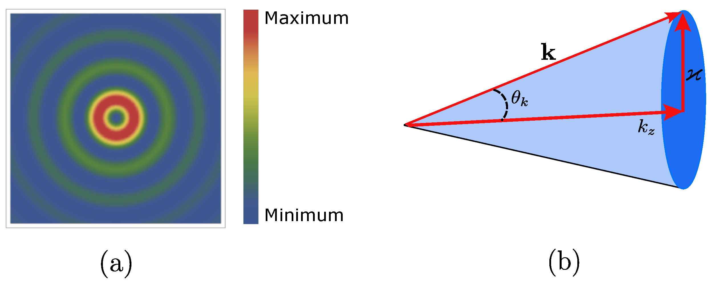
2.1. Bessel Light Modes

Bessel light modes are solutions to the Helmholtz equation in cylindrical coordinates. However, these modes do not satisfy the paraxial condition and also do not undergo diffraction as they propagate in a vacuum [8]. In addition, a twisted light mode exhibits a characteristic transverse intensity profile with multiple rings, as shown in Figure 1a. Now, we provide the vector potential of a circularly polarized Bessel light field propagating along the z axis, such that [14]

$${\mathit{A}}^{\left(\mathrm{B}\right)}(\mathit{r};m_{\gamma },\lambda )=A_0\int {\displaystyle \frac{d^2{\mathit{k}}_{\perp }}{{\left(2\pi \right)}^2}}{a}_{\varkappa m_{\gamma }}\left({\mathit{k}}_{\perp }\right){\mathit{e}}_{\mathit{k}\lambda }{e}^{i\mathit{k}·\mathit{r}},$$

(1)

where $A_0$ is constant amplitude, ${\mathit{e}}_{\mathit{k}\lambda }{e}^{i\mathit{k}·\mathit{r}}$ is the vector potential of a plane light wave, $\lambda$ is helicity, $m_{\gamma }$ is the projection of the total angular momentum and $a_{\varkappa m_{\gamma }}\left({\mathit{k}}_{\perp }\right)$ is a weight function given by

$$a_{\varkappa m_{\gamma }}\left({\mathit{k}}_{\perp }\right)={\displaystyle \frac{2\pi }{\varkappa }}{(-i)}^{m_{\gamma }}{e}^{i{m}_{\gamma }{\varphi }_k}\delta (k_{\perp }-\varkappa ).$$

(2)

Here, ${\varphi }_k$ is the azimuthal angle of the momentum vector $\mathit{k}$. Furthermore, the polarization vector can be expressed as a linear combination of the spin basis vectors ${\mathit{e}}_{m_s=\pm 1}={\displaystyle \frac{1}{\sqrt{2}}}(1,\pm i,0)$ and ${\mathit{e}}_{m_s=0}=(0,0,1)$, given by

$${\mathit{e}}_{\mathit{k}\lambda }=\sum _{m_s=0,\pm 1}{c}_{m_s}{e}^{-i{m}_s{\varphi }_k}{\mathit{e}}_{m_s}.$$

(3)

The expansion coefficient $c_{m_s}$ is given by $c_{m_s=\pm 1}={\displaystyle \frac{\pm \lambda }{\sqrt{2}}}(1\pm \lambda \cos {\theta }_k)$, $c_{m_s=0}={\displaystyle \frac{-1}{\sqrt{2}}}\sin {\theta }_k$. Furthermore, the Bessel light beam can be described as a superposition of circularly polarized plane waves ${\mathit{e}}_{\mathit{k}\lambda }{e}^{i\mathit{k}·\mathit{r}}$ with helicity $\lambda$ in momentum space, as seen in Equation (1). Moreover, the wave vectors of these plane waves with a constant transverse momentum $k_{\perp }=\varkappa$ and longitudinal momentum $k_z$ form the surface of a cone with an opening angle ${\theta }_k=\arctan (\varkappa /k_z)$ (see Figure 1b).

Although we use the integral representation of the vector potential (1) in our later calculations, it is useful to express ${\mathit{A}}_{m_{\gamma },\lambda }^{\left(\mathrm{B}\right)}\left(\mathit{r}\right)$ in the position space. This representation is particularly helpful for analyzing the polarization of a light field. To achieve this, we substitute the expression (3) into (1) and integrate over ${\varphi }_k$ using the relation ${\mathit{k}}_{\perp }·\mathit{r}=k_{\perp }{r}_{\perp }cos({\varphi }_k-{\varphi }_r)$. Additionally, the integral representation of the Bessel function [15] must be used.

$${\int }_0^{2\pi }{e}^{ila}{e}^{ix\cos (b-a)}da=2\pi i^l{e}^{ilb}{J}_l\left(x\right).$$

(4)

Then, the vector potential of the Bessel beam ${\mathit{A}}^{\left(\mathrm{B}\right)}(\mathit{r};m_{\gamma },\lambda )$ can be expressed in cylindrical coordinates ($r_{\perp },{\varphi }_r,z$) as [14]

$${\mathit{A}}^{\left(\mathrm{B}\right)}(\mathit{r}{m}_{\gamma },\lambda )=\sum _{m_s=0,\pm 1}{(-i)}^{m_s}{c}_{m_s}{J}_{m_{\gamma }-m_s}\left(\varkappa r_{\perp }\right)e^{i(m_{\gamma }-m_s){\varphi }_r}{e}^{i{k}_{z}z}{e}_{m_s}.$$

(5)

One can also treat the Bessel light fields under the paraxial approximation if one considers a smaller opening angle ${\theta }_k$. Then, one can rewrite the expansion coefficient $c_{m_s}$ as $c_{m_s=\pm 1}=\pm \lambda (1\pm \lambda \mp \lambda {\theta }_k^2/2)/2$ and $c_{m_s=0}={\displaystyle \frac{-{\theta }_k}{\sqrt{2}}}$. By incorporating the redefined expansion coefficients and limiting the summation to the leading terms $m_s=\lambda$, for which $c_{\lambda }\approx 1$, we obtain the vector potential of a circularly polarized Bessel light field as [16]

$${\mathit{A}}^{\left(\mathrm{B}\right)}(\mathit{r};m_{\ell },\lambda )={\mathit{e}}_{\lambda }{(-i)}^{\lambda }{J}_{m_{\ell }}\left(\varkappa r_{\perp }\right)e^{i{m}_{\ell }{\varphi }_r}{e}^{i{k}_{z}z}.$$

(6)

Notice that the projection of OAM $m_{\ell }$ and helicity $\lambda$ are decoupled in the vector potential of a Bessel light field in paraxial approximation (6).

2.2. Laguerre–Gaussian Light Modes

Laguerre–Gaussian modes [17] are solutions to the Helmholtz equation in cylindrical coordinates. In contrast to Bessel modes, they satisfy paraxial approximation [8]. LG modes are mainly characterized by two quantum numbers: projection of OAM $m_{\ell }$ and radial index p. As shown in Figure 2, the transverse intensity profile of the LG mode always consists of a $p+1$ number of rings. Moreover, by setting the projection of the orbital angular momentum $m_{\ell }=0$, one can obtain the well-known Gaussian beam.

Similar to the construction of the vector potential of Bessel light modes, we can write the vector potential of circularly polarized LG beams as [11]

$${\mathbf{A}}^{\left(\mathrm{LG}\right)}(\mathit{r};m_{\ell },\lambda ,p)=\int d^2{\mathit{k}}_{\perp }{v}_{p{m}_{\ell }}\left(k_{\perp }\right)e^{i(m_{\ell }+\lambda ){\varphi }_k}{\mathbf{e}}_{\mathit{k}\lambda }{e}^{i\mathbf{k}·\mathbf{r}},$$

(7)

where $v_{p{m}_{\ell }}\left(k_{\perp }\right)e^{i(m_{\ell }+\lambda ){\varphi }_k}$ is the momentum space wave function and ${\mathbf{e}}_{\mathit{k}\lambda }{e}^{i\mathbf{k}·\mathbf{r}}$ is the vector potential of a plane wave, which is circularly polarized. In the above equation, the momentum space wave function $v_{p{m}_{\ell }}\left(k_{\perp }\right)$ is given by

$$v_{p{m}_{\ell }}\left(k_{\perp }\right)={\displaystyle \frac{{(-i)}^{m_{\ell }}}{w_{\mathrm{o}}4\pi }}{e}^{-k_{\perp }^2{w}_{\mathrm{o}}^2/4}{\left({\displaystyle \frac{k_{\perp }{w}_{\mathrm{o}}}{2}}\right)}^{m_{\ell }}\sum _{\beta =0}^p{(-1)}^{\beta }{2}^{\beta +m_{\ell }/2}\left({\displaystyle \genfrac{}{}{0pt}{}{p+m_{\ell }}{p-\beta }}\right)L_{\beta }^{m_{\ell }}\left({\displaystyle \frac{k_{\perp }^2{w}_{\mathrm{o}}^2}{4}}\right).$$

(8)

In the above expression, $w_{\mathrm{o}}$ is the beam width of the LG beam at focus, also called as beam waist, $\left({\displaystyle \genfrac{}{}{0pt}{}{p+m_{\ell }}{p-\beta }}\right)$ is the binomial coefficient, and $L_{\beta }^{m_{\ell }}$ is the associated Laguerre polynomial [15]. Moreover, for simplicity, setting the radial index to $p=0$, one can further simplify the vector potential (7) as [18]

$${\mathit{A}}^{\left(\mathrm{LG}\right)}(r,\varphi ;m_{\ell },\lambda )={\left({\displaystyle \frac{2}{\pi w_{\mathrm{o}}^2\left|m_{\ell }\right|!}}\right)}^{1/2}{\left({\displaystyle \frac{r\sqrt{2}}{w_{\mathrm{o}}}}\right)}^{|m_{\ell }|}{e}^{-{\left({\displaystyle \frac{r}{w_{\mathrm{o}}}}\right)}^2}{e}^{i{m}_{\ell }\varphi }{\mathit{e}}_{\lambda }.$$

(9)

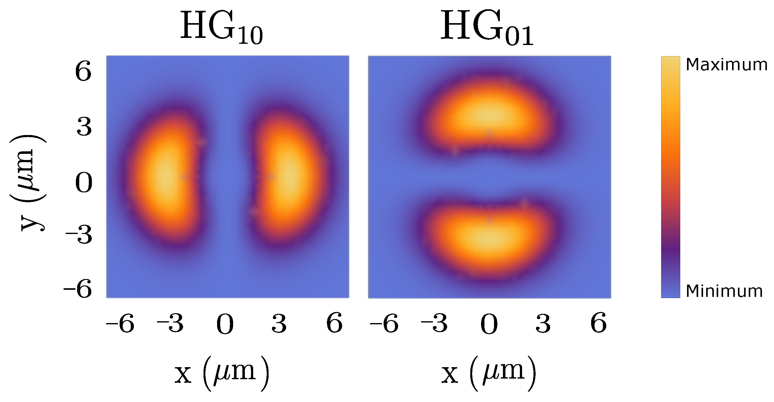
2.3. Hermite–Gaussian Light Modes

The solutions of paraxial wave equations in Cartesian coordinates are Hermite–Gaussian modes [8]. Fundamentally, HG modes are higher-order Gaussian modes. These HG modes can be characterized by two integers $m,n$, called the mode numbers. Moreover, although the intensity of HG modes is structured (see Figure 3), they do not carry orbital angular momentum like LG or Bessel modes. Since HG and LG families of beams are complete sets of functions, they can be represented in terms of each other. Thus, we express the vector potential of HG modes as

$$\begin{array}{cc}\hfill {\mathit{A}}^{{\mathrm{HG}}_{10}}\left(\mathit{r}\right)& ={\displaystyle \frac{1}{\sqrt{2}}}\left[{\mathit{A}}^{\left(\mathrm{LG}\right)}(\mathit{r};m_{\ell }=+1,\lambda =\pm 1)+{\mathit{A}}^{\left(\mathrm{LG}\right)}(\mathit{r};m_{\ell }=-1,\lambda =\pm 1)\right]\hfill \\ \hfill & \approx {\displaystyle \frac{1}{\sqrt{2}}}\left[{\mathit{A}}^{\left(\mathrm{LG}\right)}(r,\varphi ;m_{\ell }=+1,\lambda =\pm 1)+{\mathit{A}}^{\left(\mathrm{LG}\right)}(r,\varphi ;m_{\ell }=-1,\lambda =\pm 1)\right]\hfill \\ \hfill & ={\displaystyle \frac{C^{m_{\ell }}}{\sqrt{2}}}\cos \left(\varphi \right)({\widehat{\mathit{e}}}_x\pm i{\widehat{\mathit{e}}}_y),\hfill \end{array}$$

(10)

$$\begin{array}{cc}\hfill {\mathit{A}}^{{\mathrm{HG}}_{01}}\left(\mathit{r}\right)& ={\displaystyle \frac{-i}{\sqrt{2}}}\left[{\mathit{A}}^{\left(\mathrm{LG}\right)}(\mathit{r};m_{\ell }=+1,\lambda =\pm 1)-{\mathit{A}}^{\left(\mathrm{LG}\right)}(\mathit{r};m_{\ell }=-1,\lambda =\pm 1)\right]\hfill \\ \hfill & \approx {\displaystyle \frac{-i}{\sqrt{2}}}\left[{\mathit{A}}^{\left(\mathrm{LG}\right)}(r,\varphi ;m_{\ell }=+1,\lambda =\pm 1)-{\mathit{A}}^{\left(\mathrm{LG}\right)}(r,\varphi ;m_{\ell }=-1,\lambda =\pm 1)\right]\hfill \\ \hfill & ={\displaystyle \frac{C^{m_{\ell }}}{\sqrt{2}}}\sin \left(\varphi \right)({\widehat{\mathit{e}}}_x\pm i{\widehat{\mathit{e}}}_y),\hfill \end{array}$$

(11)

In the above expressions, ${\widehat{\mathit{e}}}_{x,y}$ are mutually orthogonal Cartesian unit vectors. Moreover, we have introduced the coefficient $C^{m_{\ell }}=2{\left({\displaystyle \frac{2}{\pi w_{\mathrm{o}}^2\left|m_{\ell }\right|!}}\right)}^{1/2}{\left({\displaystyle \frac{r\sqrt{2}}{w_{\mathrm{o}}}}\right)}^{|m_{\ell }|}{e}^{-{\left({\displaystyle \frac{r}{w_{\mathrm{o}}}}\right)}^2}$.

Even though LG basis is the natural choice to express HG modes, one can also use Bessel basis as discussed in ref. [19].

2.4. Linearly Polarized Structure Light Modes

As an example of a linearly polarized structure light field, we will consider linearly polarized Bessel modes. Specifically, one can write the vector potential of a Bessel light field that is linearly polarized along the x direction as

$$\begin{array}{cc}\hfill {\mathit{A}}_x^{\left(B\right)}\left(\mathit{r}\right)& ={\displaystyle \frac{i}{\sqrt{2}}}({\mathit{A}}^{\left(B\right)}(\mathit{r};m_{\gamma }=m_{\ell }+1,\lambda =+1)-{\mathit{A}}^{\left(B\right)}(\mathit{r};m_{\gamma }=m_{\ell }-1,\lambda =-1))\hfill \\ \hfill & \approx {\displaystyle \frac{i}{\sqrt{2}}}({\mathit{A}}^{\left(B\right)}(\mathit{r};m_{\ell },\lambda =+1)-{\mathit{A}}^{\left(B\right)}(\mathit{r};m_{\ell },\lambda =-1))\hfill \\ \hfill & \approx {\widehat{\mathit{e}}}_x{J}_{m_{\ell }}\left(\mathit{\varkappa }{r}_{\perp }\right)e^{i{m}_{\ell }{\varphi }_r}{e}^{i{k}_{z}z}.\hfill \end{array}$$

(12)

Notice that in the above expression, we have employed Bessel modes in a paraxial regime to obtain the vector potential expression for linear polarization. Moreover, for larger ${\theta }_k$ values, we will not obtain conventional linearly polarized Bessel modes. That is, for larger opening angles, the polarization pattern across the beam cross-section will no longer resemble a linear polarization.

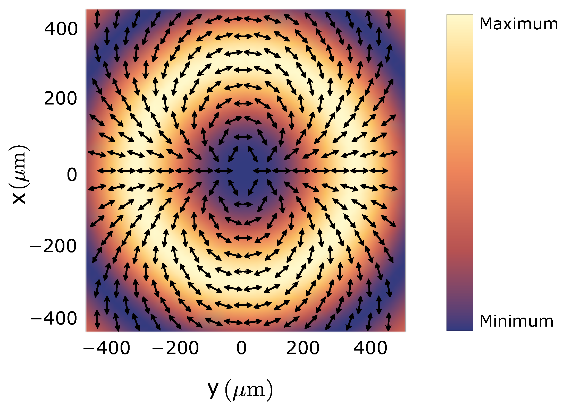
2.5. Vector Structured Light Modes

Vector light fields can be constructed in a similar fashion to a linearly polarized structured light. However, one should also vary the projection of orbital angular momentum $m_{\ell }$ of participating twisted light modes in addition to helicity $\lambda$. This results in an interplay between the phase and polarization components of twisted light modes, leading to a light field with a spatially varying polarization pattern across its beam cross-section [10].

The vector potential of a vector Bessel light field can be constructed as

$${\mathit{A}}^{\left(\mathrm{vec}\right)}\left(\mathit{r}\right)={\displaystyle \frac{1}{\sqrt{2}}}\left[{\mathit{A}}^{\left(\mathrm{B}\right)}(\mathit{r};m_{\gamma }=-1,\lambda =+1)-{\mathit{A}}^{\left(\mathrm{B}\right)}(\mathit{r};m_{\gamma }=+1,\lambda =-1)\right].$$

(13)

In the above example, we have used a specific case of $m_{\gamma }=\left|1\right|$ ($m_{\ell }=\left|2\right|$). Using (5), we can obtain an explicit expression of the above vector potential as

$$\begin{array}{cc}\hfill {\mathbf{A}}^{\left(\mathrm{vec}\right)}\left(\mathbf{r}\right)=& {\widehat{\mathit{e}}}_x{A}_0(-i)\left[{sin}^2({\theta }_k/2)J_0\left(\varkappa r_{\perp }\right)+{cos}^2({\theta }_k/2)cos\left(2\varphi \right)J_2\left(\varkappa r_{\perp }\right)\right]e^{i{k}_{z}z}\hfill \\ & +{\widehat{\mathit{e}}}_y{A}_0(-i){cos}^2({\theta }_k/2)sin\left(2\varphi \right)J_2\left(\varkappa r_{\perp }\right)e^{i{k}_{z}z}\hfill \\ \hfill & +{\widehat{\mathit{e}}}_z{A}_{0}sin{\theta }_{k}cos\varphi J_1\left(\varkappa r_{\perp }\right)e^{i{k}_{z}z}.\hfill \end{array}$$

(14)

Note that the above expression is valid for any arbitrary opening angle ${\theta }_k$. For larger values of ${\theta }_k$, the vector beam exhibits a non-zero component of the electric field along the propagation direction.

As discussed earlier, one could obtain a paraxial Bessel beam for a smaller opening angle ${\theta }_k$. Following this logic, the vector potential of a paraxial vector Bessel beam can be written by approximating (14) as

$$\begin{array}{c}\hfill {\mathbf{A}}^{\left(\mathrm{vec}\right)}\left(\mathbf{r}\right)\approx A_0(-i)\left[\cos \left(2\varphi \right){\mathit{e}}_x+\sin \left(2\varphi \right){\mathit{e}}_y\right]J_2\left(\varkappa r_{\perp }\right)e^{i{k}_{z}z},\end{array}$$

This particular vector Bessel light field exhibits a distinct polarization profile across its beam cross-section, as shown in Figure 4. Since the theory of vector light fields in LG basis is similar to that of in Bessel basis, we will not discuss it in detail here.

2.6. Transition Amplitudes

Let us consider a structured light filed of frequency $\omega$ propagating along the z axis to interact with a single ionic target. Furthermore, this ionic target placed at distance $\mathit{b}$ undergoes photoexcitation from an initial state $|{\alpha }_i{J}_i{M}_i\rangle$ to a final state $|{\alpha }_f{J}_f{M}_f\rangle$. For this particular process, we can write the transition amplitude as

$$M_{fi}=\langle {\alpha }_i{J}_i{M}_i|\mathit{\alpha }·\mathit{A}\left(\mathit{r}\right)|{\alpha }_f{J}_f{M}_f\rangle ,$$

(15)

where $\mathit{\alpha }$ is the Dirac matrix [20] and $\mathit{A}\left(\mathit{r}\right)$ is the vector potential of the interacting light field.

In this subsection, we will provide a detailed derivation of the transition amplitude for circularly polarized Bessel modes interacting with an atomic target. Using this, we will illustrate how to construct transition amplitudes for linearly polarized and vector Bessel modes.

2.6.1. Bessel Light Modes

If the interacting radiation is a structured light in Bessel basis, then transition amplitude becomes

$$M_{fi}^{\left(\mathrm{B}\right)}=\langle {\alpha }_f{J}_f{M}_f|\mathit{\alpha }·{\mathit{A}}^{\left(B\right)}(\mathit{r};m_{\gamma },\lambda )|{\alpha }_i{J}_i{M}_i\rangle .$$

(16)

Before continuing, it is practical to represent the plane wave components present in the vector potential of the Bessel light field using the angular momentum basis. That is, we perform a multipole expansion of the plane wave vector potential to obtain [21,22]

$${\mathit{A}}_{\mathit{k}\lambda }^{\left(\mathrm{pl}\right)}\left(\mathit{r}\right)=\sum _{\mathbb{M}M}\sqrt{2\pi }{\left(i\right)}^L{(2L+1)}^{1/2}{\left(i\lambda \right)}^p{D}_{M\lambda }^L({\varphi }_k,{\theta }_k,0){\mathit{a}}_{LM}^p\left(\mathit{r}\right),$$

(17)

where $D_{M\lambda }^L({\varphi }_k,{\theta }_k,0)=e^{-iM{\varphi }_k}{d}_{M\lambda }^L$ is the Wigner D function, M is the projection of total angular momentum, and $\mathbb{M}=(L,p)$ is the multipole parameter. This parameter depends on the total angular momentum of radiation L and $p=1$ ($p=0$) denotes the electric (magnetic) multipole component. Furthermore, ${\mathit{a}}_{LM}^p\left(\mathit{r}\right)$ represents the vector spherical harmonics of rank L.

Since the transverse intensity profile of a structured light beam is non-uniform, the position of the ionic target is critical. Therefore, we multiply the vector potential of the structured light by displacement operator $e^{-i\mathit{k}·\mathit{b}}$, where $\mathit{b}=(b,{\varphi }_b,0)$ denotes the distance between the atomic target and the beam axis. The transition amplitude after performing the integration over $d{\mathit{k}}_{\perp }$ can be written as

$$\begin{array}{cc}\hfill M_{fi}^{\left(\mathrm{B}\right)}\left(\mathit{b}\right)& =\sum _{\mathbb{M}M}\sqrt{2\pi }{\left(i\lambda \right)}^p{(2L+1)}^{1/2}{i}^{L-M}{e}^{i(m_{\gamma }-M){\varphi }_b}{J}_{m_{\gamma }-M}\left(\varkappa b\right)d_{M\lambda }^L\left({\theta }_k\right)\hfill \\ \hfill & {(2J_f+1)}^{-1/2}\langle J_i{M}_i,LM|J_f{M}_f\rangle \langle {\alpha }_f{J}_f\left|\right|\mathit{\alpha }·{\mathit{a}}_L^p\left(\mathit{r}\right)\left|\right|{\alpha }_i{J}_i\rangle ,\hfill \end{array}$$

(18)

where we have employed the Wigner–Eckart theorem [21]; $\langle {\alpha }_f{J}_f{M}_f|\alpha ·{\mathit{a}}_{LM}^{\Lambda }|{\alpha }_i{J}_i{M}_i\rangle =\langle J_i{M}_i,LM|J_f{M}_f\rangle {(2J_f+1)}^{-1/2}\langle {\alpha }_f{J}_f\left|\right|\mathit{\alpha }·a_L^{\Lambda }\left|\right|{\alpha }_i{J}_i\rangle$. This helps us to separate the geometrical and atomic parameters in the transition amplitude. That is, the Clebsch–Gordan coefficients $\langle J_i{M}_i,LM|J_f{M}_f\rangle$ characterize the geometrical parameters of the transition amplitude, and the reduced transition amplitude $\langle {\alpha }_f{J}_f\left|\right|\mathit{\alpha }·{\mathit{a}}_L^p\left(\mathit{r}\right)\left|\right|{\alpha }_i{J}_i\rangle$ describes the atomic parameters. This reduced transition amplitude can be obtained using the atomic computation package Jena Atomic Calculator (JAC) [23]. That is, all bound-state wave functions that are required are generated within JAC self-consistently, based on the Hartree–Fock–Slater potential. Later, these ab initio wave functions are utilized to evaluate the (many electron) transition amplitudes of electron–photon interactions using the standard angular reduction of symmetry-adapted configuration state functions [24]. The benefits and use of these symmetry-adapted functions have been summarized recently [25] and show how JAC helps to expand the atomic theory towards new light beams and applications.

Furthermore, one can utilize the transition amplitude to obtain an expression for the total rate of excitation as follows:

$$W_{fi}={\displaystyle \frac{2\pi }{(2J_i+1){\alpha }^2}}\sum _{M_i{M}_f}{\left|M_{fi}^{\left(B\right)}\left(\mathit{b}\right)\right|}^2.$$

(19)

where $\alpha$ is the fine structure constant. Moreover, in the above expression, one has to average over initial projection $M_i$ and summation over final projection $M_f$. One can also write an expression for a relative sub-level population of the excited state with the help of transition amplitude as follows:

$${\sigma }_r={\displaystyle \frac{{\left|M_{fi}^{\left(\mathrm{B}\right)}\left(b\right)\right|}^2}{{\sum }_{M_f}{\left|M_{fi}^{\left(B\right)}\left(b\right)\right|}^2}}.$$

(20)

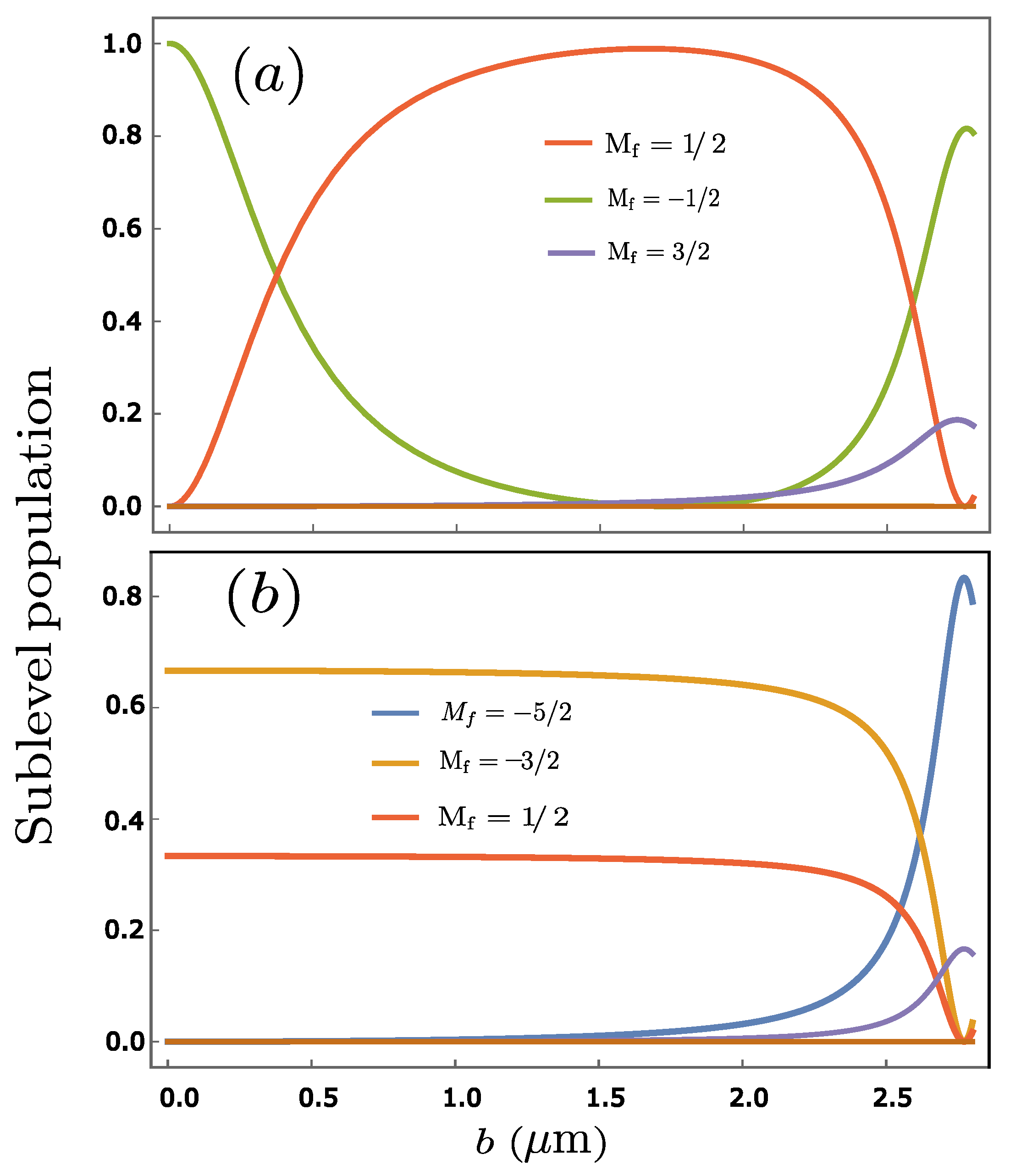
2.6.2. Vector Structured Light Modes

Furthermore, if the interacting light is a vector Bessel beam, then the transition amplitude can be written using (18)

$$M_{fi}^{\left(\mathrm{vec}\right)}\left(\mathit{b}\right)={\displaystyle \frac{1}{\sqrt{2}}}\left[M_{fi}^{\left(B\right)}(\mathit{b};m_{\gamma }=+1,\lambda =-1)-M_{fi}^{\left(\mathrm{B}\right)}(\mathit{b};m_{\gamma }=-1,\lambda =+1)\right].$$

(21)

2.6.3. Linearly Polarized Structured Light Modes

The transition amplitude for a linearly polarized Bessel light field interacting with the target atom can be written using (18)

$$M_{fi;\mathrm{linear}}^{\left(\mathrm{B}\right)}\left(\mathit{b}\right)={\displaystyle \frac{i}{\sqrt{2}}}\left[M_{fi}^{\left(B\right)}(\mathit{b};m_{\gamma }=m_{\ell }-1,\lambda =-1)-M_{fi}^{\left(\mathrm{B}\right)}(\mathit{b};m_{\gamma }=m_{\ell }+1,\lambda =+1)\right].$$

(22)

Similarly, one can construct a transition amplitude for HG and LG light modes interacting with an ionic target, as discussed in [19,26].

3. Discussion and Conclusions

Even though our theoretical framework developed in the last section can consider any ionic target, we will choose the Ca⁺ ion to illustrate this. For this purpose, we will consider circularly polarized and linearly polarized Bessel light fields interacting with the target ion. To be specific, we will consider a 789 nm light field to interact with a Ca⁺ ion such that it undergoes an electric quadrupole transition from $4s{}_{\mathrm{}}{}^2{S}_{1/2}_{\mathrm{}}^{\mathrm{}}\to 3d{}_{\mathrm{}}{}^2{D}_{5/2}_{\mathrm{}}^{\mathrm{}}$ atomic states. For this particular system, we will discuss the relative partial cross-section of the excited state population.

In the first instance, let us consider the incoming radiation to be a circularly polarized Bessel light field. For this light field, if the Ca⁺ ion is placed on the beam axis, then it will undergo a transition between an initial $|4S_{1/2},M_i=-1/2\rangle$ to a final state $|3D_{5/2},M_f=-1/2\rangle$ (see Figure 5). On the other hand, if the ionic target is displaced from the beam axis, then we will observe an atomic transition between an initial $|4S_{1/2},M_i=-1/2\rangle$ to a final state $|3D_{5/2},M_f=1/2\rangle$, as shown in Figure 5.

Position-dependent atomic transitions can be better understood using the angular momentum selection rule $M_i+M=M_f$. Specifically, from (18), it is evident that the $J_{m_{\gamma }-M}\left(\varkappa b\right)$ term determines the value of M across the beam cross-section of structured light beam. For instance, if the target ion is positioned on the beam axis, where $b=0$, then

$$J_{m_{\gamma }-M}\left(0\right)={\delta }_{m_{\gamma }-M,0}.$$

(23)

That is, on the beam axis, only atomic transitions satisfying the selection rule $M_i+m_{\gamma }=M_f$ are allowed. Thus, we observe an atomic transition between an initial $|4S_{1/2},M_i=-1/2\rangle$ to a final state $|3D_{5/2},M_f=-1/2\rangle$ (see Figure 5). On the other hand, if the atomic target is displaced from the beam axis by a distance of b, then the projection of total angular momentum M can take all possible values between $-L$ and $+L$.

Now, let us assume the interacting radiation to be a linearly polarized Bessel beam. For this scenario, if the target ion is positioned on the beam axis, then one observes that two atomic transitions are possible. However, the transition from an initial $|4S_{1/2},M_i=-1/2\rangle$ to a final state $|3D_{5/2},M_f=-3/2\rangle$ is more probable, as seen in Figure 5. Furthermore, for larger b values, we observe a transition from an initial $|4S_{1/2},M_i=-1/2\rangle$ to a final state $|3D_{5/2},M_f=-5/2\rangle$ (see Figure 5).

To summarize our discussion so far, we have explored various structured light beams in terms of their intensity profiles and polarization patterns using their vector potentials. We then derived the transition amplitude for a structured light field interacting with a single ionic target using the first-order perturbation theory. Specifically, we provided a detailed derivation for a Bessel light field interacting with a single target ion. Using this amplitude, we constructed transition amplitudes for linearly and vector-polarized Bessel light beams. To illustrate this, we examined the photoexcitation of a single ionic target by circularly and linearly polarized Bessel light beams. In particular, we focused on electric quadrupole transitions in a Ca⁺ ion driven by the selected structured light fields. With our results, we analyzed the sub-level population of the excited atomic state and its dependence on the parameters of an incoming structured light field. In particular, it should be noted that these results for circularly and linearly polarized Bessel light fields are calculated for the first time, as previous works have considered LG [11] and vector LG beams [26]. However, these results re-confirm the position-dependent atomic transitions observed in previous works [11,27] with the Ca⁺ ion interacting with structured light fields. Moreover, these results help us to better understand non-dipole atomic transitions driven by structured light fields, enabling us to build better atomic clocks and quantum information processing devices.

References

1. Erhard, M.; Fickler, R.; Krenn, M.; Zeilinger, A. Twisted photons: New quantum perspectives in high dimensions. Light. Sci. Appl. 2018, 7, 17146. [Google Scholar] [CrossRef] [PubMed]
2. Heintzmann, R.; Gustafsson, M.G.L. Subdiffraction resolution in continuous samples. Nat. Photonics 2009, 3, 362–364. [Google Scholar] [CrossRef]
3. Simpson, N.B.; Allen, L.; Padgett, M.J. Optical tweezers and optical spanners with Laguerre–Gaussian modes. J. Mod. Opt. 1996, 43, 2485–2491. [Google Scholar] [CrossRef]
4. Souza, C.E.R.; Borges, C.V.S.; Khoury, A.Z.; Huguenin, J.A.O.; Aolita, L.; Walborn, S.P. Quantum key distribution without a shared reference frame. Phys. Rev. A 2008, 77, 032345. [Google Scholar] [CrossRef]
5. Kotlyar, V.; Kovalev, A.; Porfirev, A.; Kozlova, E. Orbital angular momentum of a laser beam behind an off-axis spiral phase plate. Opt. Lett. 2019, 44, 3673–3676. [Google Scholar] [CrossRef] [PubMed]
6. Padgett, M.; Courtial, J.; Allen, L. Light’s Orbital Angular Momentum. Phys. Today 2004, 57, 35–40. [Google Scholar] [CrossRef]
7. Marrucci, L.; Manzo, C.; Paparo, D. Optical Spin-to-Orbital Angular Momentum Conversion in Inhomogeneous Anisotropic Media. Phys. Rev. Lett. 2006, 96, 163905. [Google Scholar] [CrossRef] [PubMed]
8. Andrews, D.L.; Babiker, M. The Angular Momentum of Light; Cambridge University Press: Cambridge, UK, 2012. [Google Scholar]
9. Wang, J.; Castellucci, F.; Franke-Arnold, S. Vectorial light–matter interaction: Exploring spatially structured complex light fields. AVS Quantum Sci. 2020, 2, 031702. [Google Scholar] [CrossRef]
10. Gbur, G.J. Singular Optics; CRC Press: Boca Raton, FL, USA, 2016. [Google Scholar]
11. Peshkov, A.A.; Seipt, D.; Surzhykov, A.; Fritzsche, S. Photoexcitation of atoms by Laguerre-Gaussian beams. Phys. Rev. A 2017, 96, 023407. [Google Scholar] [CrossRef]
12. Afanasev, A.; Carlson, C.E.; Solyanik, M. Atomic spectroscopy with twisted photons: Separation of M1–E2 mixed multipoles. Phys. Rev. A 2018, 97, 023422. [Google Scholar] [CrossRef]
13. Afanasev, A.; Carlson, C.E.; Mukherjee, A. High-multipole excitations of hydrogen-like atoms by twisted photons near a phase singularity. J. Opt. 2016, 18, 074013. [Google Scholar] [CrossRef]
14. Matula, O.; Hayrapetyan, A.G.; Serbo, V.G.; Surzhykov, A.; Fritzsche, S. Atomic ionization of hydrogen-like ions by twisted photons: Angular distribution of emitted electrons. J. Phys. At. Mol. Opt. Phys. 2013, 46, 205002. [Google Scholar] [CrossRef]
15. Abramowitz, M.; Stegun, I.A. Handbook of Mathematical Functions with Formulas, Graphs, and Mathematical Tables; US Government Printing Office: Washington, DC, USA, 1948; Volume 55. [Google Scholar]
16. Schulz, S.A.L.; Peshkov, A.A.; Müller, R.A.; Lange, R.; Huntemann, N.; Tamm, C.; Peik, E.; Surzhykov, A. Generalized excitation of atomic multipole transitions by twisted light modes. Phys. Rev. A 2020, 102, 012812. [Google Scholar] [CrossRef]
17. Allen, L.; Beijersbergen, M.W.; Spreeuw, R.J.C.; Woerdman, J.P. Orbital angular momentum of light and the transformation of Laguerre-Gaussian laser modes. Phys. Rev. A 1992, 45, 8185–8189. [Google Scholar] [CrossRef] [PubMed]
18. Peshkov, A.A.; Bidasyuk, Y.M.; Lange, R.; Huntemann, N.; Peik, E.; Surzhykov, A. Interaction of twisted light with a trapped atom: Interplay between electronic and motional degrees of freedom. Phys. Rev. A 2023, 107, 023106. [Google Scholar] [CrossRef]
19. Peshkov, A.A.; Jordan, E.; Kromrey, M.; Mehta, K.K.; Mehlstäubler, T.E.; Surzhykov, A. Excitation of Forbidden Electronic Transitions in Atoms by Hermite–Gaussian Modes. Ann. Phys. 2023, 535, 2300204. [Google Scholar] [CrossRef]
20. Johnson, W.R. Lectures on Atomic Physics; Notre Dame University Department of Physics: Notre Dame, Indiana, 2006. [Google Scholar]
21. Rose, M.E. Elementary Theory of Angular Momentum; Courier Corporation: North Chelmsford, MA, USA, 1995. [Google Scholar]
22. Brink, D.M.; Satchler, G.R. Angular Momentum; Oxford University Press: Oxford, UK, 1994. [Google Scholar]
23. Fritzsche, S. A fresh computational approach to atomic structures, processes and cascades. Comput. Phys. Commun. 2019, 240, 1–14. [Google Scholar] [CrossRef]
24. Gaigalas, G.; Fritzsche, S.; Grant, I.P. Program to calculate pure angular momentum coefficients in jj-coupling. Comput. Phys. Commun. 2001, 139, 263–278. [Google Scholar] [CrossRef]
25. Fritzsche, S. Application of Symmetry-Adapted Atomic Amplitudes. Atoms 2022, 10, 127. [Google Scholar] [CrossRef]
26. Ramakrishna, S.; Hofbrucker, J.; Fritzsche, S. Photoexcitation of atoms by cylindrically polarized Laguerre-Gaussian beams. Phys. Rev. A 2022, 105, 033103. [Google Scholar] [CrossRef]
27. Schmiegelow, C.T.; Schulz, J.; Kaufmann, H.; Ruster, T.; Poschinger, U.G.; Schmidt-Kaler, F. Transfer of optical orbital angular momentum to a bound electron. Nat. Commun. 2016, 7, 12998. [Google Scholar] [CrossRef] [PubMed]
Figure 1. (a) The transverse intensity profile of a Bessel beam, displaying an infinite number of rings with an opening angle of θ k = 10 ° and m γ = 0 . (b) Representation of Bessel beams as a coherent superposition of plane waves with wave vectors k confined to the surface of a cone with an opening angle θ k in momentum space.
Atoms 13 00020 g001
Figure 2. The transverse intensity profile of the LG beam.
Atoms 13 00020 g002
Figure 3. The transverse intensity profiles of circularly polarized HG modes, HG10 (left) and HG01 (right), with a beam waist of 3 μm.
Atoms 13 00020 g003
Figure 4. The intensity and polarization of the vector Bessel beam. Here, m = ± 2 , and the opening angle is set to θ k = 0 . 11 ° .
Atoms 13 00020 g004
Figure 5. Relative sub-level population for the electric quadrupole transition 4 s S 1 / 2 2 3 d D 5 / 2 2 in the Ca+ ion. The interacting light field is assumed to comprise (a) circularly and (b) linearly polarized Bessel beams of wavelength 789 nm, m γ = 0 , θ k = 10 ° . The ionic target is assumed to be prepared in the ground state | 4 S 1 / 2 , M f = 1 / 2 and is displaced from the beam axis by b.
Atoms 13 00020 g005
Disclaimer/Publisher’s Note: The statements, opinions and data contained in all publications are solely those of the individual author(s) and contributor(s) and not of MDPI and/or the editor(s). MDPI and/or the editor(s) disclaim responsibility for any injury to people or property resulting from any ideas, methods, instructions or products referred to in the content.