1. Introduction
Resonant magneto-optics and the related field of atomic magnetometry have a history that started in the late 1950s with the research of Dehmelt [
1] and Bell and Bloom [
2,
3] stretching to the 1960s, particularly with the work of Cohen-Tannoudji [
4,
5]. The following decades brought important progress in the comprehension of optical pumping phenomena [
6,
7] and prepared the conditions for an important revival at the beginning of the current century [
8], which was inspired by numerous attracting applications and facilitated by technological progress.
Most of the application fields envisaged for atomic magnetometers were identified on the basis of their excellent sensitivity, and, in the case of radio-frequency magnetometers, on their response to high-frequency fields. In addition to their use as state-of-the-art detectors in fundamental physics experiments [
9], among these application fields emerges the detection of bio-magnetism, e.g., in the construction of magneto-encephalographs [
10,
11], magneto-cardiographs [
12,
13,
14], and magneto-miographs [
15]. Another promising area is represented by nuclear magnetic resonance in ultra-low (e.g., at microtesla level) or even vanishing fields, where atomic magnetometers find use as non-inductive detectors [
16,
17,
18,
19,
20], and also in imaging experiments [
21,
22,
23,
24]. Radio-frequency magnetometers find other interesting applications in the detection and imaging of eddy currents [
25,
26], with implications in non-destructive testing of materials [
27], security [
28], and bio-medicine [
29]. Further perspectives originate from the possibility of producing miniaturized sensors [
30,
31,
32,
33] and arranging them in arrays [
34].
There exists a variety of atomic magnetometers, which are nowadays also produced as commercial devices. However, they all share several common features [
35]. Generally, the working principle consists of using (near) resonant light to orient atoms in a long-lived state (or to induce alignment or higher order momenta); making atoms evolve in the magnetic field under measurement, which thus imprints its features in the subsequent state; and eventually interrogating the atomic sample by means of probe radiation that characterizes its optical (absorptive/dispersive) behavior.
The above mentioned three-step (pumping–evolution–interrogation) procedure [
36] can be performed in sequence or simultaneously. Numerous interaction geometries (e.g., the relative orientation of the field, pump beam, and probe beam) can be considered, tailored time-dependent fields can be applied, various approaches (absorption, dispersion, and polarimetry) can be used at the interrogation stage, etc. A
plethora of configurations can be proposed and this large variety comes with wide ranges of sensitivity, bandwidth, dynamical range, time and space resolution, etc.
An interesting implementation consists of pumping atoms synchronously with their precession around a (nearly) static field. In this case, the pumping radiation must be modulated (in terms of amplitude, polarization, or wavelength) and the probe radiation detects a time-dependent optical behavior. Such a light-modulated setup was firstly proposed by Bell and Bloom [
2], who used amplitude-modulated light from a caesium discharge lamp.
The ideal (optimal) configuration of a Bell-and-Bloom setup considers a static magnetic field oriented transversely with respect to the pump radiation wave vector. This causes the resonantly induced macroscopic magnetization to precess in a plane perpendicular to . This precession can be analyzed by probe radiation propagating in that plane. The Faraday rotation effect offers a favorable detection scheme based on polarimetric measurements; the probe radiation is linearly polarized and the polarization plane is rotated by an angle that oscillates at the precession frequency. The amplitude of this oscillation is maximized when the pumping radiation is modulated at the Larmor frequency set by the static field, i.e., at an atomic magnetic resonance.
If the pump modulation frequency is fixed, small and slow variations in the static field bring the system to a near-resonant condition, with the typical effects of signal reduction and dephasing, the latter being more effectively and easily detected, thanks to its (nearly) linear dependence on the detuning, i.e., on the difference between the frequency at which the pump radiation is modulated and the precession frequency set by the field under measurement.
This classical picture of Bell-and-Bloom behavior applies when the field variation is small compared with the magnetic resonance linewidth and slow with respect to the relaxation time of the atomic orientation. Most of the literature reporting Bell-and-Bloom magnetometers interprets the detected signals in terms of such quasi-static and near-resonant conditions [
37], furthermore considering the optimal field orientation. In other terms, the field is usually assumed to be (nearly) perpendicular to the pump and probe propagation, (nearly) time independent, and (nearly) matching the Larmor resonant condition. This paper aims to provide a general analysis of the behavior of a Bell-and-Bloom magnetometer when it operates in the presence of a generic time-dependent field that is parallel to the static (bias) one.
The availability of a more accurate model is of relevance when the output of a magnetometer is used as an error signal to implement feedback-based field stabilization systems [
38,
39,
40,
41,
42], as well as when designing feed-forward ones [
43] or when evaluating the effects of strong stray fields, which is of particular relevance for systems operating in unshielded environments [
11,
44].
This paper is organized as follows. In
Section 2, we describe the mathematical approaches used to solve the Larmor equation under the generic conditions mentioned above. In
Section 3, we report the numerical findings of the model, while the main outcomes are discussed in
Section 4 and some conclusions are drawn in
Section 5.
2. Model
Our aim is to examine the dynamics of spins precessing in a time-dependent magnetic field considering the case of a Bell-and-Bloom magnetometer as sketched in
Figure 1. The figure represents a light-modulated magnetometer, in which two laser beams (pump and probe) co-propagate in an atomic vapor in the presence of a time-dependent, transversely oriented magnetic field. The pump beam is modulated and constitutes a time-dependent forcing term that produces a macroscopic magnetization in the medium. This magnetization precesses around the magnetic field and its evolution is detected as a Faraday rotation of the probe beam polarization. A detailed model of the considered spin dynamics enables a more accurate interpretation of the acquired signals. In particular, it helps highlight features that emerge due to the parametric nature of the considered system and that, as we will show, can play a crucial role, particularly in the presence of strong and/or fast varying fields. The starting point in modeling of the spin response is the equation of motion (Larmor equation) for the magnetization vector
:
Here, the constant rate
accounts for any relaxation mechanism (assumed isotropic for simplicity),
is the action of the forcing term obtained through optical pumping (see [
45] for details),
is the gyromagnetic factor, and
is the applied magnetic field. Finally,
is the magnetic torque experienced by the magnetization vector.
In this paper, we are interested in a configuration where the pumping light and the magnetic field are orthogonal. We chose the
x axis along the pump (so
) and the
y axis along the magnetic field, which, in turn, is composed of a static
and a time-dependent
part. Introducing the frequencies
and
, the relevant Larmor equation becomes
where
, and we are interested in
, which is the quantity related to the Faraday rotation of the probe laser collinear with the pump as, for example, in [
45,
46].
The solution of (
2), which is a first-order, linear, non-homogeneous, and parametric differential equation, can be written as
where we introduce the Larmor angle associated with the time-dependent field:
We assume that both the forcing and the time-dependent field are real-valued periodic functions that can be expressed in terms of Fourier series. Namely, we assume that the forcing term oscillates with period
and the time-dependent field oscillates with period
:
and we can set
(or otherwise redefine
), obtaining that
is also a periodic function, which permits us to write
where the
coefficients are complicated functions of
. It is worth noting that the
coefficients are related to the Bessel functions of the first kind in the case of a purely sinusoidal time-dependent field.
Now, the steady-state (SS) solution, valid for
, of (
3) becomes
which can be simplified by taking into account that, under usual experimental conditions, the pumping frequency is (nearly) resonant with the Larmor frequency set by the static field, that is,
, resulting in
where we introduced the detuning
and implicitly defined the
coefficients and the
complex function.
We would like to point out that result (
8) has a more general validity; indeed, it is valid also when the experimental apparatus tracks the component at the fundamental frequency of the pumping modulation. In fact, in this case, the approximation is valid just because this is the term singled out by the measuring apparatus. The validity of the approximation in the resonant case (
) comes from the fact that the singled out term is the biggest one in the sum over
m.
After this demodulation, the quantity monitored is the phase of
, which is still a periodic function:
where, in general, the
coefficients can be evaluated only numerically as
A notable exception is the case of a low-intensity time-dependent field which is discussed in the following.
Low-Intensity Limit
When the time-dependent field is small with respect to the static one, which in our formalism means that the
coefficients are small quantities, i.e.,
, where
is a small positive quantity, the Larmor angle becomes
, a small quantity too. It follows that
and
,
for
. Substituting this in the first line of (
8), one obtains
Considering that the second term in parentheses is
and that
for small
, one obtains for the phase
:
Here, the first term is just a constant offset which depends also, through the coefficient
, on the precise characteristics of the pump modulation signal. We disregard this term because it does not contain information about the dynamical field encoded in the
coefficients. The next term, the first order in
in this perturbation theory, contains relevant information, and after some algebra, can be rewritten as
which is identical to the expression reported in [
47] and can be recast as the output of a linear system
3. Results
The result reported in (
8) is quite general and applies to a complicated time dependence of
which would require the consideration of many
parameters, as well as of the case of a simple sinusoidal oscillation.
It is worth to point out that in the phase time signal (Equation (
9)), the coefficient
gives only a constant contribution which amounts to an experimental offset and can be safely neglected, resulting in an experimental advantage because one does not need to take into account the precise form of the pumping signal. This is not the case if one chooses to monitor the modulus of
, where the
coefficient enters in a multiplicative way. This can be seen by inspection, noting that
can be rewritten as
and then
As a result of the complicated dependence of the
coefficients on
, it is difficult to draw valid conclusions for arbitrary values of the parameters. In such a sense, the analytical low-intensity limit of Equation (
12) is a nice result, which allows a discussion in terms of linear time-invariant systems. However, in this paper, we explore the complementary regime, presenting results obtained as explained in the previous section.
To be more concrete, we fix the time dependence as a simple cosine, namely,
, so that
are the Bessel functions of first kind and the coefficients
can be written as
and we expect that for not-so-small
, the higher-harmonic coefficients
will also become important. In fact, the system is a parametric one and it will show a kind of “non-linear” behavior. In other terms, even for a simple sinusoidal time-dependent field as “input”, higher order harmonics will appear in the monitored phase.
In the following pictures, we present numerical results for the first Fourier coefficients of the phase for different values of the amplitude of the time-dependent field. The reported simulations use only adimensional parameters to simplify as much as possible the physical discussion and to make the plots applicable to systems characterized by diverse values of . We choose to use as the relevant frequency scale.
In
Figure 2,
Figure 3,
Figure 4 and
Figure 5, the modulus of
(from left to right) is reported as a function of
for fixed values of
, respectively. Each curve represents a different value of the detuning
in units of
.
As can be seen in
Figure 2, where
, the perturbative limit of Equation (
13) applies. In fact,
and
are two and three orders of magnitude smaller than
, respectively. However, as can be seen in
Figure 3,
Figure 4 and
Figure 5,
and
become increasingly comparable in magnitude with
when the amplitude
of the time-dependent field is increased.
Let us consider the behavior of
for different values of
. For small
, the curve can be interpreted as the response of a low-pass filter, while when increasing
it resembles a band-pass filter centered in
. This point of view is reinforced in the low
regime by the result of Equation (
13). However, as can be seen in the pictures, this interpretation can be pushed also for higher values of
even if some structure starts appearing close to
.
The behavior of is more structured. For (we observed this for all the even coefficients ), a “low-pass” profile evolves into a double peaked structure with the highest peak centered around and the other around . Increasing gives rise to a small structure close to .
Similar conclusions can be drawn for ; here, the number of visible peaks is three even for small . It seems reasonable to assume that this is the general behavior of the coefficients , i.e., increasing increases both the number of “relevant” and for each the number of visible peaks are centered at .
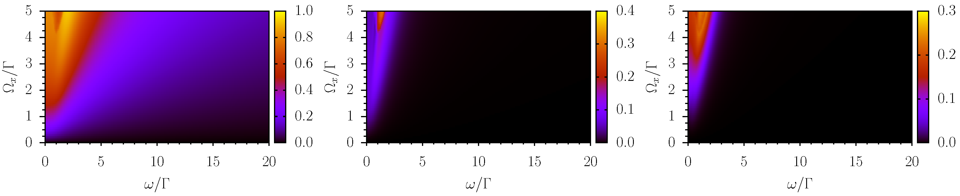
An alternative and complementary visualization of the described phenomenology is reported in
Figure 6 and
Figure 7. In these maps, the modulus of the signals at
,
, and
(from left to right) is mapped as a function of the frequency (horizontal axes) and amplitude (vertical axes) of the time-dependent field. The two figures refer to cases of small detuning (low pass behavior) and large detuning (band pass behavior), respectively.
4. Discussion
The main scope of this paper is to investigate the dynamic response of a Bell-and-Bloom system to a time-dependent field parallel to the bias one. This subject is often presented in terms of an approximation, the validity of which requires that the time-dependent field is small and varies slowly with respect to relaxation time and that the pumping radiation is modulated in resonance with the precession frequency set by the dominant static field. Under these stringent but frequently fulfilled conditions, the systems permits a simplified treatment and behaves as a linear forced-damped oscillator with a low-pass (Butterworth filter) response [
10,
48].
We have previously analyzed the behavior of such a system using a perturbative approach in the amplitude of the time-dependent field [
47] in a more general configuration, as a generic orientation of the field was considered. Before discussing the results presented in
Section 3, it is worth recalling the main outcomes obtained with that approach.
Apart from the basic physical interest to characterize and model spin dynamics in a time-dependent field, our study can help interpret the recorded magnetometric signals more accurately. In particular, it provides a quantitative evaluation of the harmonic distortion that occurs with increasing field variations and allows us to evaluate the distortions in the time domain caused by a frequency-dependent signal phase shift. The latter is particularly relevant when the magnetic signals contain broad spectrum characteristics, as in the case of traces with sharp edges or spikes.
4.1. Perturbative Results
An interesting feature resulting from the first-order perturbative approximation emerges when the pump radiation is modulated at a frequency detuned from the exact resonance. Under this condition, the simplified low-pass response becomes inadequate and a band-pass behavior is observed, with an enhanced response to AC components at frequencies close to the pump frequency detuning
, as also observed in ref. [
42].
In application, this feature may help tailor the system response to the detection of oscillating terms at frequencies around . For instance, a magnetometer with a resonance as narrow as 20 Hz maybe used to detect an AC field oscillating at 200 Hz with a good efficiency, provided that the pump light is modulated at a frequency 200 Hz away from .
An interesting behavior is obtained at an intermediate detuning, . This condition produces a nearly flat amplitude response up to a cut-off frequency set by . Such an extended flat bandwidth is obtained at the expense of a slight reduction in the signal amplitude, if compared to the case. Concerning the phase of the magnetometric signal, a maximally extended constant phase (non dispersive) response is instead achieved under the condition .
In this first-order approximation, the precessing spins do not respond to field variations along direction perpendicular to the static field; such a response appears in the next order. Indeed, the perturbative treatment developed in [
47] shows that the second-order approximation predicts terms that
double and
mix the frequencies at which time-dependent fields are applied. It is worth noting that frequency mixing among diverse components of the time-dependent field comes with several peculiar features and it does not occur among all the couples of components, as detailed in [
47].
A further increase in the time-dependent field also makes the second-order approximation inadequate and the numerical analysis developed in
Section 2 becomes necessary. For the sake of simplicity, in this work, the time-dependent field is considered at arbitrarily high amplitudes, but only along the bias field direction. Moreover, the presented results are obtained with a single-frequency term, so that no frequency mixing occurs and the non-linearities are pointed out in terms of a harmonic analysis.
4.2. Non-Perturbative Results
The numerical analysis performed at a rather weak intensity is perfectly consistent with the first-order perturbative analysis recalled in
Section 4.1. In particular, the leftmost plot in
Figure 2 shows that at resonance (
), the system has a low-pass response, which evolves into an extended flat response when
and becomes a band-pass one for
. At large detunings (band-pass regime), the peak response is half the maximum observed at low frequency and vanishing detunings. A harmonic analysis shows that in the low-field regime (
), the anharmonicity of the response is negligible. A close inspection of the vertical scales in
Figure 2 highlights that the second and third harmonic terms (
) are depressed by two and three order of magnitudes with respect to the fundamental one, respectively.
Figure 3 and
Figure 4 show the effects of a moderate increase in the amplitude of the time-dependent field. Under conditions in which
, the low-pass and band-pass behavior does not change appreciably, while the anharmonicity becomes progressively more evident, e.g., for
, the third harmonic peaks observed at large detunings are only one order of magnitude weaker than the fundamental one.
The results obtained at small and moderate amplitudes of the time-dependent field (
Figure 2,
Figure 3 and
Figure 4) show pretty similar features in the spectral response, and the main difference concerns only the anharmonicity level. The response observed for large
is characterized by a peak at
for all harmonic terms. However, the second harmonic term (
) also has a secondary peak at
and an additional peak at
emerges for the third harmonic term,
.
Figure 5 shows new spectral features in the responses. Strong time-dependent fields cause extra peaks to emerge in the plots. In particular, the leftmost plot (
) of
Figure 5 shows the appearance of an extra peak at
.
The maps shown in
Figure 6 and
Figure 7 confirm the analysis reported above. In these figures, it can be seen that the amplitudes of higher harmonics (
) become comparable to that of the fundamental tone
for large values of
(
), and that they have a more structured dependence on
. In addition, it can be observed that both the fundamental tone and the higher harmonics peak at
and that secondary peaks appear at sub-harmonics in the case of
and
.
5. Conclusions
We studied the effect of a time-dependent magnetic field on the Bell-and-Bloom magnetometer in the configuration in which the time-dependent magnetic field is parallel to the bias static one. We generalized the analysis beyond the quasi-static and low-amplitude regime usually found in the literature, unveiling interesting features such as confirming the low-pass to band-pass transition for a large amplitude of the time-dependent field. Moreover, for large amplitudes of the time-dependent field, the emergence of the “non-linear” behavior of the system is demonstrated.
Our findings may be of interest to improve the accuracy of the interpretation of magnetometric measurements, in particular to evaluate their harmonic distortion, and to better reconstruct magnetic signals characterized by relatively broad spectra. The analysis of the response to large field variations covers a phenomenology that is normally overlooked in applied research, as the latter is often focused on the detection of weak signals. Furthermore, it highlights and characterizes the non-linear features that can contaminate the measurement when strong stray field disturbances are superimposed on the weak signals under investigation. An interesting outcome consists of a feature that is observed when the detuning is progressively increased; correspondingly, the response of the system evolves from the well-known low-pass behavior to band-pass behavior. This latter can be of great relevance, for instance, when noise spectra are experimentally recorded to evaluate system performance and specifically sensitivity profiles.


