Role of Simple Spatial Gradient in Reinforcing the Accuracy of Temperature Determination of HED Plasma via Spectral Line-Area Ratios

Abstract

We report on the simulation of temperature gradients in tamped NaFMgO target-foil plasma, heated and backlit by z-pinch dynamic hohlraum radiation. Our approach compares the spectroscopic output of a collisional-radiative model (prismspect) with soft X-ray absorption spectra collected on Sandia National Laboratories’ (SNL) Z Pulsed Power Facility. The pattern of minimum ${\chi }^2$ is seen to agree with an efficient, three-parameter model. Results show that a negligible gradient in electron temperature $T_e$ is consistent with experimental data, justifying the assumptions of previous work. The predicted sensitivity of line spectra to the gradient-aligned profile of $T_e$ is documented for each spectral feature, so that the line-area ratio between a pair of spectral features may be assessed as a proxy for the existence and quantification of such gradients.

1. Introduction

The need for accurate diagnosis of the temperature and density of a high-energy-density (HED) plasma via spectroscopic means is well-reported [1,2,3]. In particular, to study the characteristics of massive accretors such as X-ray binaries or active galactic nuclei (AGN), the astrophysical community relies on the analysis of emission from the associated accretion-powered plasma [4]. Such distant, photoionized plasmas pose a formidable challenge to models and have provided an insight into where theories must improve [5].

When confronted with these complex systems, it is quite reasonable to exclude effects due to inhomogeneity and/or non-stationarity for simplicity. Indeed, numerical experiments have buttressed the validity of these assumptions in particular regimes. In ref. [6], for example, the authors conclude that corrections due to spatial temperature gradients are negligible for all transitions with wavelength $\lambda >12.5$ Å, which exceeds the highest wavelength of interest. Unfortunately, recent work [7] asserts that an assumption of stationarity is ill-founded in many scenarios involving HED plasma. Moreover, a systematic investigation of the effect of spatial gradients on spectroscopic diagnoses of temperature and density has not yet been explored.

In this study, we implement the collisional-radiative model prismspect [8] to construct synthetic absorption spectra, which are subsequently compared with data gathered from the Z Facility at SNL. In line with previous work that utilized line-area ratios to infer electron temperature in a radiatively-heated NaFMgO plasma [9,10], we investigate the robustness of line-area ratios in the presence of spatial gradients.

Specifically, when these ratios compare relatively high-energy atomic transitions to low-energy transitions (e.g., Mg He-$\gamma$ to F He-$\gamma$), we observe monotonic functions of temperature difference $\Delta T$. This relationship may provide a spectroscopic diagnosis for spatial gradient magnitude, though knowledge of the average electron temperature $\langle T_e\rangle$ must be known a priori. For the reason that $\langle T_e\rangle$ is likely to also be inferred via line-area ratios, it is paramount to categorize the sensitivity of these ratios to changes in both $T_e$ and $\nabla T_e$.

Effectively, this report is an extension of line-ratio techniques documented in refs. [9,10,11] and elsewhere. Section 2 outlines the experimental set-up, while Section 3 details our hypothesis and various methods of data reduction. Section 4 provides a discussion of the implications and applications of our work.

2. Materials and Methods

The experiments were performed on the Z Facility at SNL [12], using the Z Pinch Dynamic Hohlraum (ZPDH) [13], under the auspices of the Z Astrophysical Plasma Properties (ZAPP) collaboration [14]. As the materials and methods have been documented elsewhere [9,10], we provide only a summary of the experimental scenario. In particular, the ZPDH consists of a 120 tungsten wire array with an inner diameter of 20 mm, nested in a 240 tungsten wire, 40 mm diameter array [14]. A cylindrical, 6 mm diameter, 14.5 mg/cm${}^3$ CH${}_2$ foam fits in the center of the inner array [15]. Current in excess of 26 MA, provided by discharging 36 Marx capacitor banks in parallel [16], flows through the wire arrays over a 100 ns interval, with peak current lasting approximately 3 ns [10]. Driven by the $\mathbf{J}\times \mathbf{B}$ force, ablated tungsten streams towards the z-pinch axis until stagnation, driving a radiating shock through the foam [15]. Due to the high opacity of the tungsten plasma, the shock radiation is trapped, effectively creating a hohlraum [9,15]. Crucially, this “dynamic” hohlraum can facilitate total X-ray energy and power exceeding 1.5 MJ and 200 TW, respectively [14,17].

The target foil was mounted 2.65 cm from the z-pinch cylindrical axis, glued directly to the Return Current Can (RCC) (see Figure 1). This configuration furnishes the minimum distance from the pinch axis, which also leaves intact the implicit azimuthal symmetry.

Each target was fabricated to have 4 $\mu$m of parylene (C${}_8$H${}_8$) tamper on both the front and back sides of 10 repeated double-deposition layers of sodium fluoride/magnesium-oxide foil. The NaF and MgO deposition layers were interleaved within the foil to enhance plasma homogeneity upon expansion [17] (see Figure 2). Foil elements have been chosen with similar atomic numbers ($Z=8,9,11,12$), to minimize the ionization energy required to observe similar charge-state configurations. The oxygen was inadvertently introduced as an impurity during foil fabrication.

Absorption spectra are resolved and collected by a time-integrated convex-crystal spectrometer (TIXTL) [18]. The TIXTL consists of two spectrometer arms, one with a 4-inch convex, spherically-bent potassium acid phthalate (KAP) crystal and the other with a 4-inch convex, spherically-bent rubidium acid phthalate (RAP) crystal. In this study, we focus exclusively on data derived from the KAP crystal (i.e., $\lambda$ = 7–15 Å, $h\nu \approx$ 800–1800 eV). Although the spectrometer is time-integrated, the majority of the signal comes from radiative flux during the 3 ns stagnation, when the pinch is hot and dense enough to produce a large quantity of X-rays (we discuss the likelihood of temporal gradients in Section 4). The TIXTL has a resolving power of $\lambda /\Delta \lambda \sim 900$ in the 7–15 Å  range, and is spatially resolving with respect to the axial direction of the pinch. Kodak 2924 X-ray film was used to record the absorption spectra.

3. Results

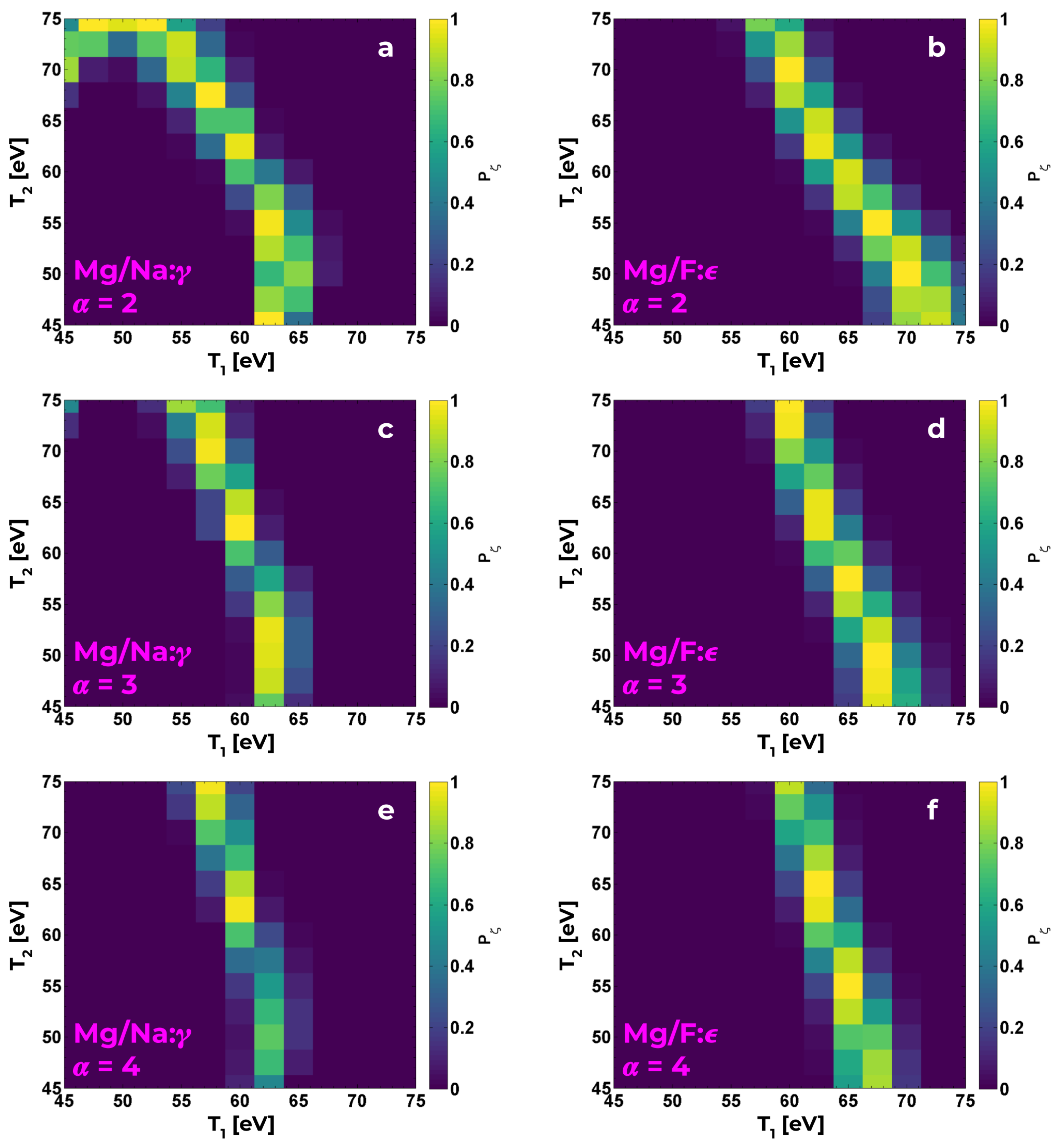
3.1. Description of Gradient Model

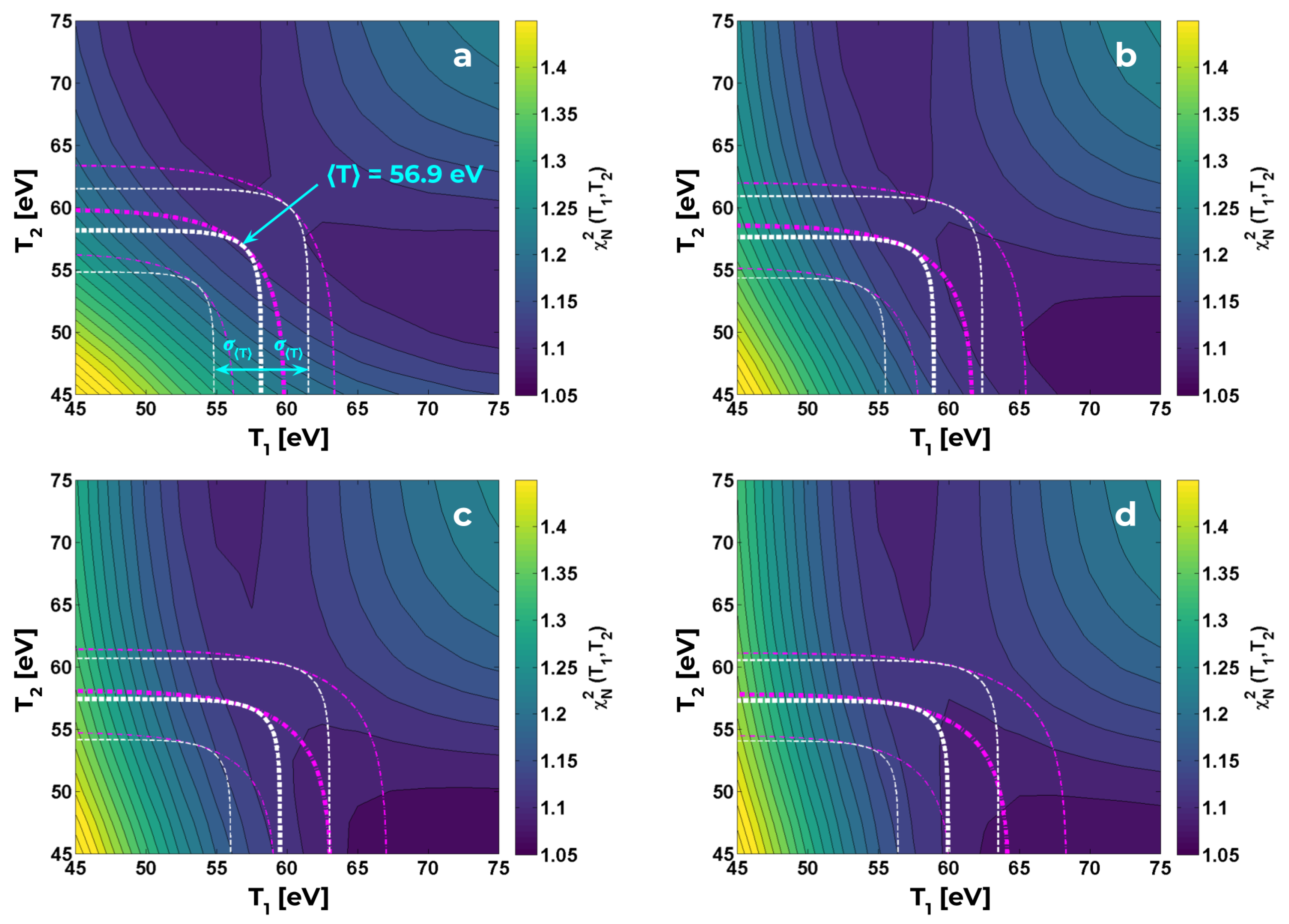
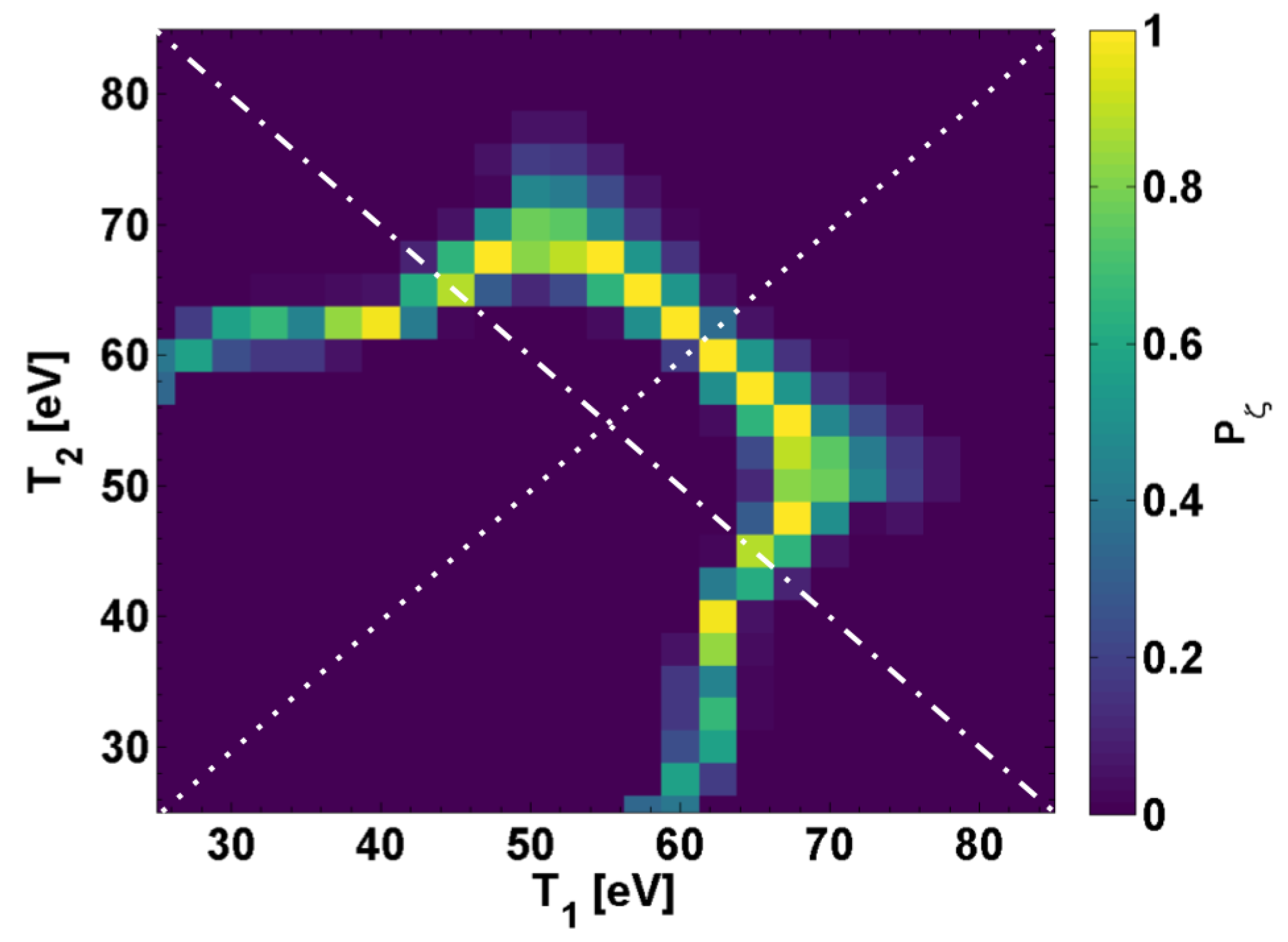
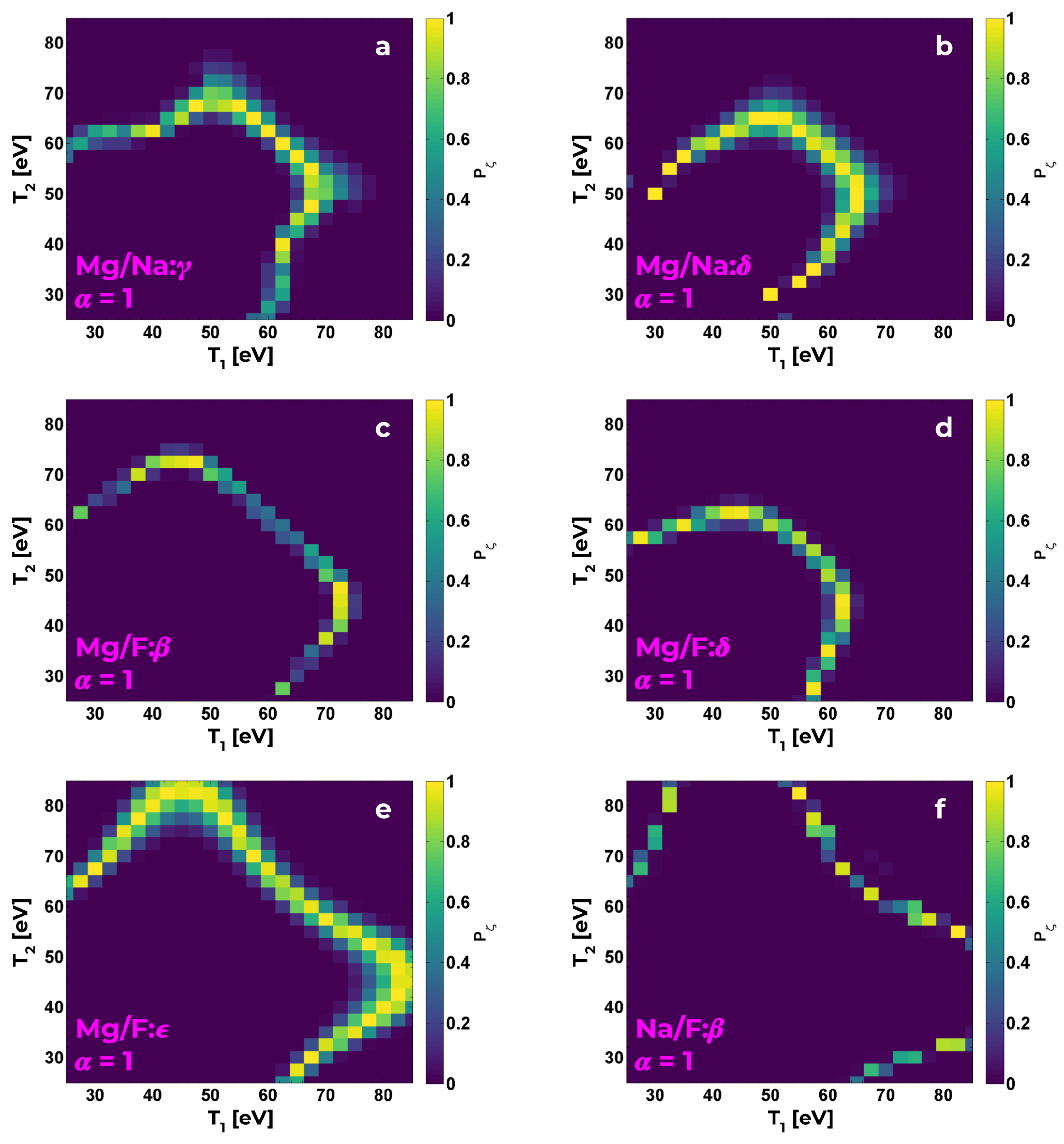
We hypothesize a simple, three-parameter schema for the electron temperature profile across the target-foil plasma. The model parameters are two temperatures, $T_{e,1}$ and $T_{e,2}$, in conjunction with the length ratio $L_2/L_1$, where $L_k$ represents the length of the interval in which the temperature is assumed to be constant and equal to $T_{e,k}$ (see Figure 3). In essence, we investigate the likelihood of a thin, hot layer on the pinch-facing side of the target-foil plasma. Preliminary work with prismspect, using the more general case of 10 temperatures, predicted a best-fit temperature profile with these characteristics. However, because this may be an artifact of a time-varying temperature, we are motivated to perform the more careful analysis herein. To best reproduce the experimental conditions, we demand that the total length $L\equiv L_1+L_2$ conforms to the measured size of the NaFMgO layer, thus $L=3494$ Å [10].

The temperatures $T_{e,1}$ and $T_{e,2}$ are used as inputs to prismspect in order to compare them with experimental data. The range for both temperatures is 45–75 eV, in steps of 2.5 eV; ion density was fixed at $n_i=1.75\times {10}^{20}$ ions/cc. These values are chosen to reflect the results presented in refs. [9,10]. Guided by previous work [4,5,6,9,10,15,17,19,20,21,22], we model our system as 1D, both for simplicity and efficiency. This assumption is reasonable due to the negligible lateral gradients in temperature and density, as two laterally displaced points on the foil see effectively analogous radiation. The use of a 3 mm × 3 mm limiting aperture, placed between the foil and the imaging slit (see Figure 1), serves to reduce edge effects and further justify a 1D simulation. Additionally, we assume local thermodynamic equilibrium (LTE) [1,23]; prior investigations of similar atomic transitions and comparable regimes of temperature and density [17,19,21] imply that the collisional ionization rates are sufficient to validate this assumption. While prismspect incorporates bound-bound, bound-free, and free-free transitions, only bound-bound transitions will be considered when comparing them to the relative (continuum-normalized) transmission obtained from the experiment.

To account for the possibly unequal lengths $L_1$ and $L_2$, we vary the areal density ${\rho }_{{}_A,k}=\rho L_k$ in each simulation, where $\rho$ is the mass density of the foil. Explicitly, the areal density of the experimental foil is found to be

$$\begin{array}{cc}\hfill {\rho }_{{}_A,\exp }& =\rho L\hfill \\ \hfill & =[\left(6.13\right)m_{\mathrm{Na}}+\left(6.74\right)m_{\mathrm{F}}+\left(6.74\right)m_{\mathrm{Mg}}+\left(5\right)m_{\mathrm{O}}]\times {10}^{17}{\mathrm{cm}}^{-2}\hfill \\ \hfill & \approx 85\mathsf{\mu }\mathrm{g}/{\mathrm{cm}}^2,\hfill \end{array}$$

where $m_x$ is the atomic mass of element x (in amu), and the values of areal abundance are adduced by Rutherford backscattering [10,24,25]. Thus, to simulate a foil with an integral length ratio of $L_2/L_1\equiv \alpha \in \mathbb{N}$, we use the areal densities.

$$\begin{array}{cc}\hfill {\rho }_{{}_A,1}& =\frac{L_1{\rho }_{{}_A,\exp }}{L_1+L_2}=\frac{{\rho }_{{}_A,\exp }}{\alpha +1},\hfill \\ \hfill {\rho }_{{}_A,2}& =\frac{L_2{\rho }_{{}_A,\exp }}{L_1+L_2}=\frac{\alpha {\rho }_{{}_A,\exp }}{\alpha +1}.\hfill \end{array}$$

(1)

Once both prismspect runs are completed for a given length ratio, the simulated transmission ${\mathcal{T}}_{\mathrm{PS}}$ is found using ${\mathcal{T}}_{\mathrm{PS}}={\mathcal{T}}_1{\mathcal{T}}_2,$ where ${\mathcal{T}}_k$ represents the transmission through a foil with areal density ${\rho }_{{}_A,k}$. In this state, the simulated absorption spectra lack the instrument broadening incurred by the experimental data. To account for this, the simulated transmission is convolved with a measured instrument function [20], which incorporates broadening due to finite source size, spectrometer uncertainty, and film limitations [10]. The final simulated transmission is therefore [15]

$${\mathcal{T}}_{\mathrm{sim}}\left(\lambda \right)={\int }_{-\infty }^{\infty }d{\lambda }^{\prime }g(\lambda -{\lambda }^{\prime }){\mathcal{T}}_{\mathrm{PS}}\left({\lambda }^{\prime }\right),$$

(2)

where $g\left(\lambda \right)$ is the instrument function, and ${\mathcal{T}}_{\mathrm{PS}}\left(\lambda \right)$ is assumed to be zero outside the range $7\le \lambda \le 15$ Å. Figure 4 provides a direct comparison of the experimental and simulated absorption; it is clear from inspection that the modeled amplitudes, relative positions, and line-widths compare well with observation.

Exposed experimental film was digitized and processed in the manner outlined by [9,10]. In short, after alignment, adjustment for film fog, division by continuum emission from the ZDPH, and interpolation, experimental data is given by a single function of transmission $\mathcal{T}$ versus wavelength (see Figure 4). This absorption spectrum contains, in principle, all the information required to effectively infer both the electron temperature $T_e$ (from line-area ratios) and the ion density $n_i$ (from line broadening) [9,15]. In ref. [9], analysis of isoelectronic line-area ratios determined the electron temperature of a MgFNaO target-foil plasma, fielded on Z Machine shot Z2950, to be $T=56.9\pm 3.2$ eV (hereafter we drop the subscript on $T_e$).

3.2. ${\chi }^2$ Minimization

The estimation of the experimental electron temperature profile is informed by chi-squared analysis. Specifically, we use the reduced ${\chi }^2$ statistic [26]

$${\chi }_N^2=\frac{1}{N-1}\sum _{k=1}^N\frac{{\left[{\mathcal{T}}_{\exp }\left({\lambda }_k\right)-{\mathcal{T}}_{\mathrm{sim}}\left({\lambda }_k\right)\right]}^2}{{\sigma }_{\mathcal{T}}^2\left({\lambda }_k\right)},$$

(3)

where ${\mathcal{T}}_{\exp }$ and ${\mathcal{T}}_{\mathrm{sim}}$ are the experimental and simulated transmissions, respectively, and ${\sigma }_{\mathcal{T}}$ is the standard deviation of the experimental data, each for a given wavelength ${\lambda }_k$. When ${\mathcal{T}}_{\mathrm{sim}}$, derived from prismspect output, is a good fit of the experimental data, the reduced ${\chi }^2$ statistic tends to unity, ${\chi }_N^2\sim 1$.

Fixing a value of the length ratio $L_2/L_1$, we calculate the reduced chi-squared statistic for each pair of temperatures $T_1$ and $T_2$, leading to a 2D map ${\chi }_N^2(T_1,T_2)$. Figure 5 illustrates the evolution of this map as $L_2/L_1$ varies from 1 to 4. Of particular salience is the goodness-of-fit in all cases. Across the entire temperature range of interest, ${\chi }_N^2$ varies only slightly, from approximately 1.05 to 1.5. This implies the effect of temperature gradients is subtle, in line with the findings of [6].

For clarity, we overlay curves representing the average temperature $\langle T\rangle =56.9$ eV and the corresponding uncertainty $\langle T\rangle \pm {\sigma }_{\langle T\rangle }$, as found via isoelectronic line-area ratios in ref. [9]. Despite ostensibly neglecting the results of inter-stage line-area ratio analysis (see Section 3.3), we will find in Section 3.4 that a spatial temperature gradient is not likely in either case. To compensate for the unequal distribution of temperature, we use the Boltzmann distribution $p=exp(-E/T)/\mathcal{Z}$, where p is the population density of emitters with energy E and $\mathcal{Z}$ is the partition function. The average population density of emitters $\langle p\rangle$ along a line of sight is then

$$\langle p\rangle \approx \frac{L_1{e}^{-E/T_1}+L_2{e}^{-E/T_2}}{L_1+L_2}=e^{-E/\langle T\rangle },$$

(4)

where we assume the differences in charge state distribution are not sufficient to appreciably alter the individual partition functions. Hence, the average temperature for a given transition energy E is calculated by the

$$\langle T\rangle =-\frac{E}{ln\left(e^{-E/T_1}+\alpha e^{-E/T_2}\right)-ln\left(1+\alpha \right)},$$

(5)

using length ratio $\alpha \equiv L_2/L_1$. For a known $\langle T\rangle$, the best-fit temperature profile is inferred by the minimum of ${\chi }_N^2(T_1,T_2)$ along a curve of constant $\langle T\rangle$. Broadly speaking, this analysis reports an increase in the likelihood of a spatial temperature gradient as the ratio $L_2/L_1$ increases. For example, in Figure 5d, we see that a temperature difference ($\Delta T\equiv T_1-T_2$) on the order of 10 eV is consistent with ${\chi }_N^2$ analysis for low-energy transitions ($\sim 800$ eV); this is not observed in Figure 5a,b.

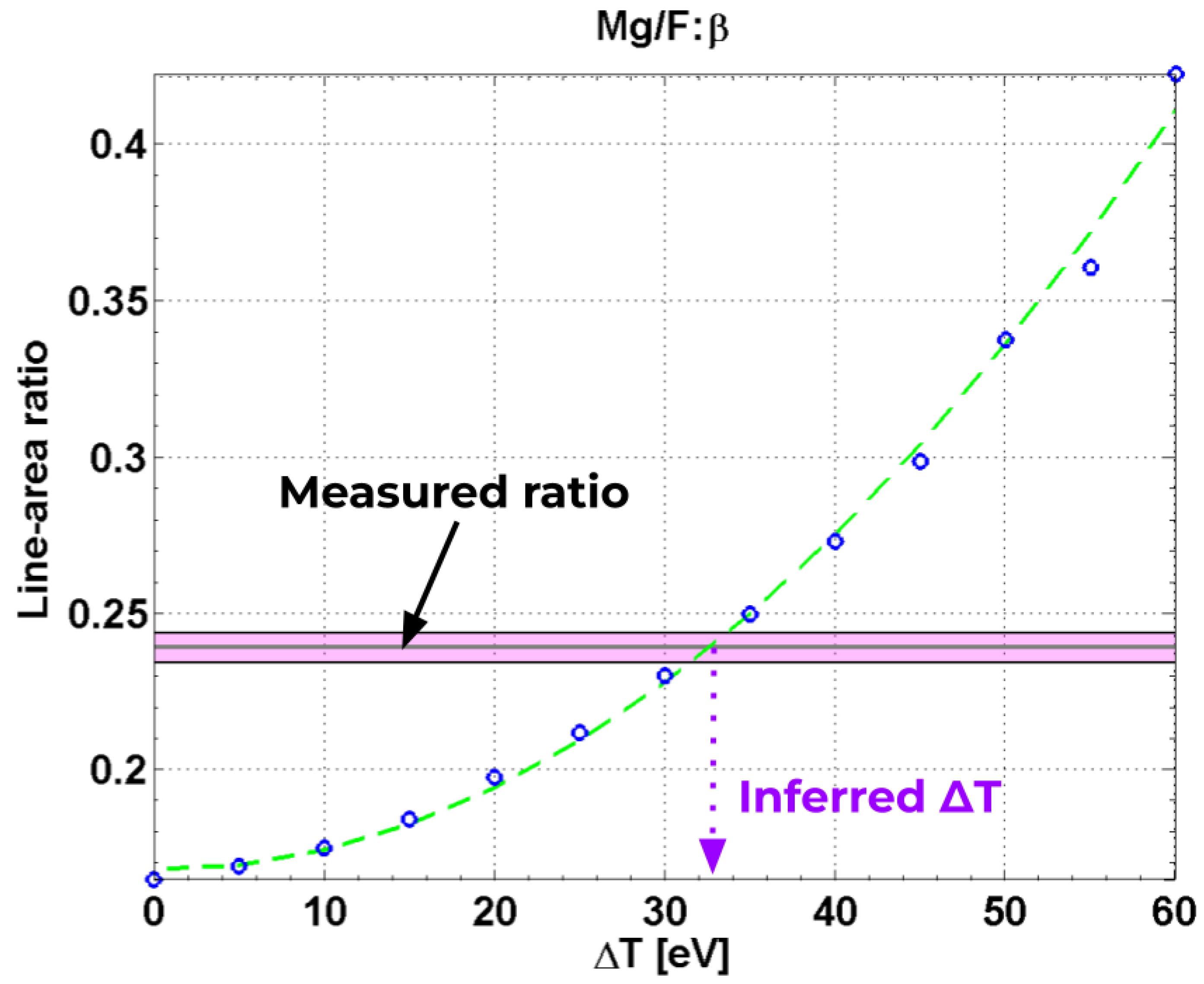
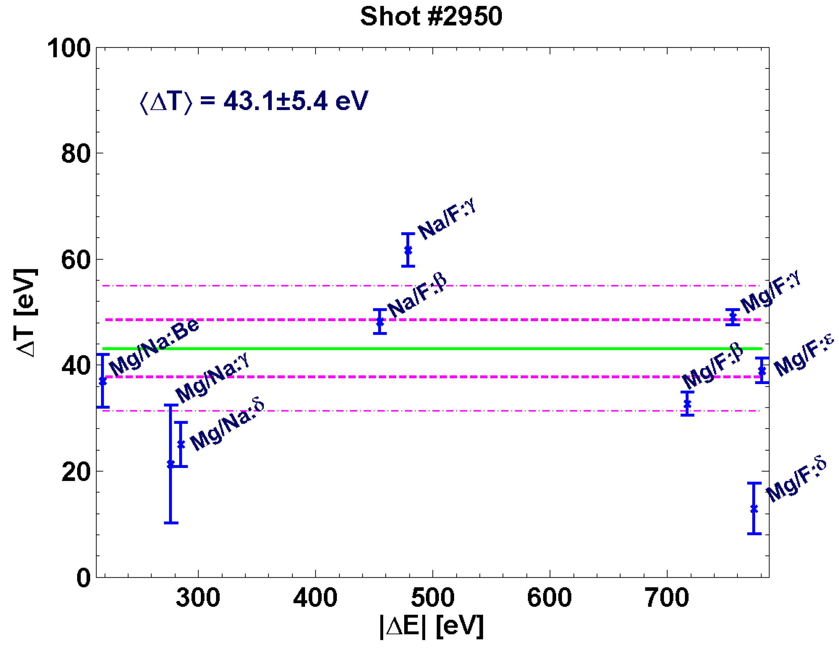
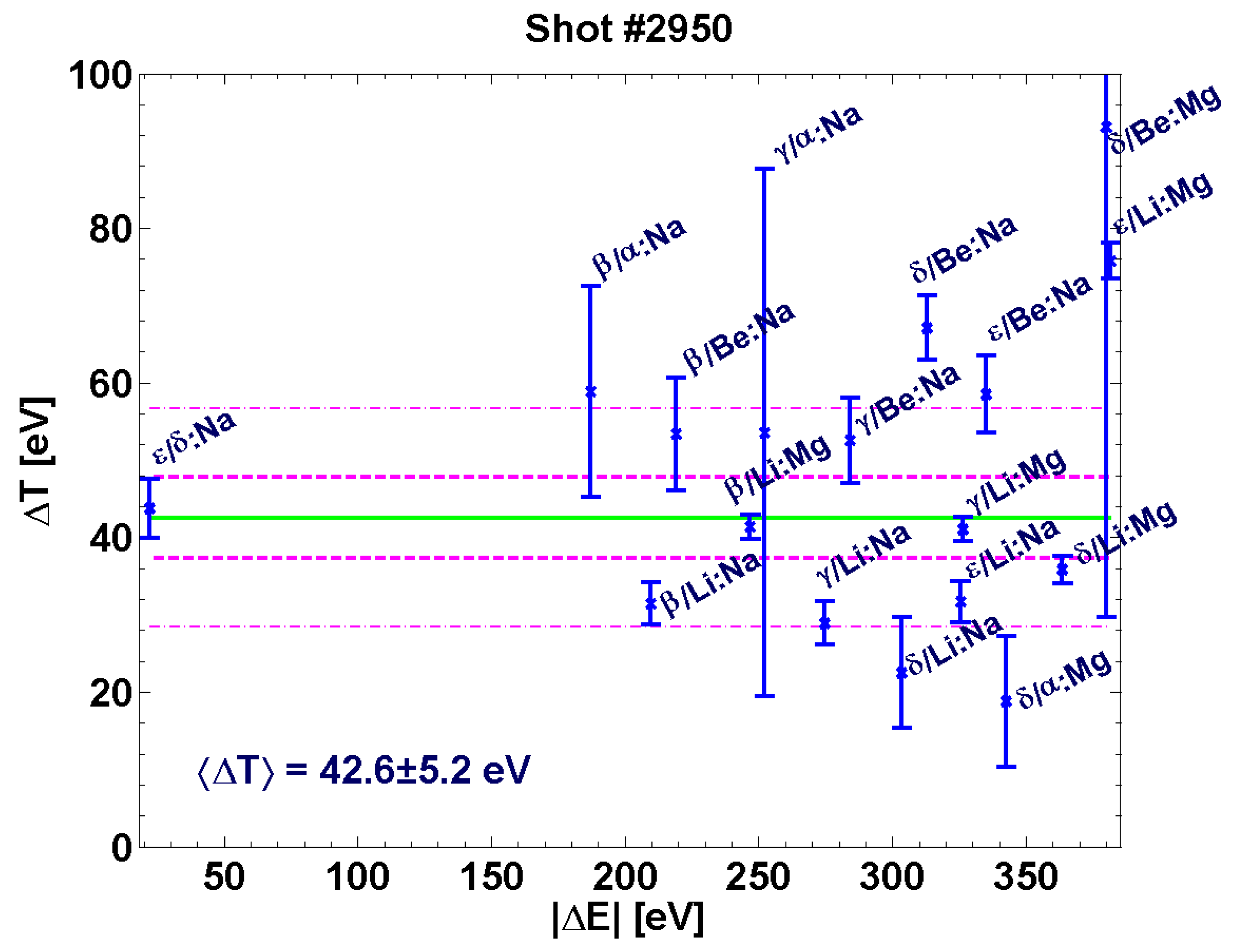
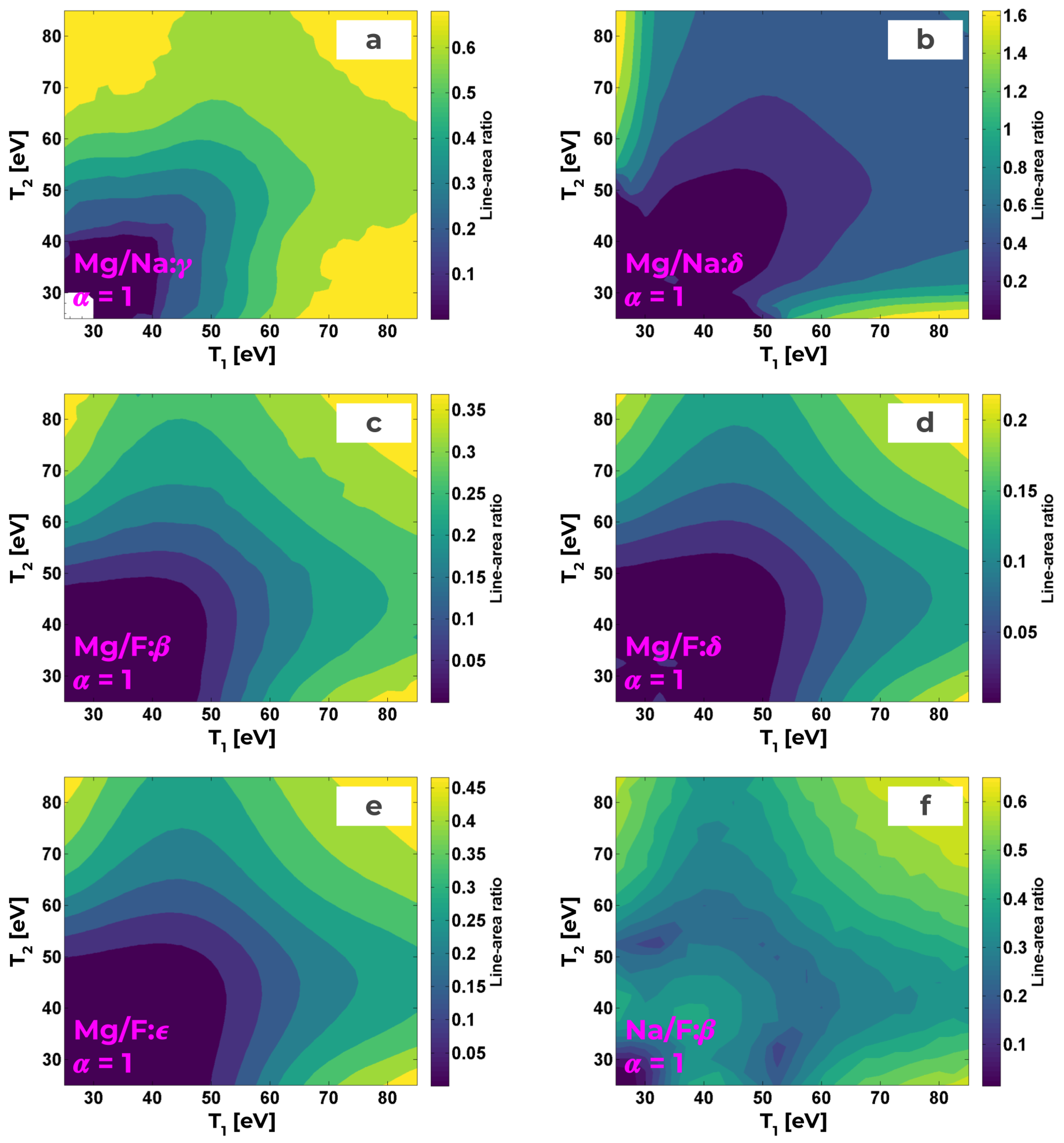
3.3. Quantitative Assessment via Line-Area Ratios

In this subsection, quadratic regression is employed to constrain the value of $\Delta T$. As in previous analyses [9,10], we convert all absorption spectra (both simulated and experimental) to optical depth $\tau$, using $\tau =-log\mathcal{T}$. Generally, optical depth is a function of wavelength. For a given bound-bound transition with a lower state l and an upper state u, we have

$${\tau }_{lu}\left(\lambda \right)\propto p_l{\varphi }_{lu}\left(\lambda \right),$$

(6)

where ${\varphi }_{lu}$ is the lineshape of the transition, and $p_l$ is the population density of the lower state [15]. Integrating over wavelength, and using $\int {\varphi }_{lu}d\lambda =1$, we find

$$\int {\tau }_{lu}d\lambda \propto p_l.$$

(7)

Thus, the integrated area of a particular spectral feature (in optical depth) provides a measurement of population density. Within each charge state, energy levels are distributed according to the Boltzmann relation $p_{\mathrm{excited}}/p_{\mathrm{ground}}\propto exp(-\Delta E/T)$ [15], so increases in electron temperature facilitate the population of higher energy levels. This constitutes the crux of the line-area ratio diagnostic.

Once transmission data are converted to optical depth, each prominent spectral feature is fitted with a pseudo-Voigt profile [27], which is integrated to provide a value of line-area. Despite work demonstrating that more detailed line shapes are superior to Voigt functions (e.g., [19]), the pseudo-Voigt maximizes computational efficiency while also accounting for Stark and Doppler broadening [10,22] (see Figures 7 and 8 in ref. [9] for examples of typical Voigt fits). Pairs of line-areas are formed into ratios, which may be categorized as either isoelectronic or inter-stage. Isoelectronic ratios compare similar electronic transitions in different elements (e.g., Mg He-$\delta$ and F He-$\delta$) [11], while inter-stage ratios compare different transitions within the same element (e.g., Na He-$\beta$ and, Na He-$ϵ$) [28].

Plotting line-area ratios determined from prismspect data as a function of $\Delta T$, we observe monotonic behavior (see Figure 6). For simplicity, we fix the value of $(T_1+T_2)/2=55$ eV, which, in view of (5), implies that $\langle T\rangle$ varies as we adjust $\Delta T$. Performing a quadratic least-squares fit [26] to each simulated ratio yields an invertible function that delineates the inferred value of $\Delta T$, based on the measured value of the line-area ratio (cf. Section 4 in [9]). Figure 6 elucidates this procedure for the line-area ratio of Mg He-$\beta$ to F He-$\beta$.

Each ratio furnishes a value of temperature change and an associated standard error (i.e., $\Delta T_k\pm {\sigma }_k$). We calculate the weighted mean and unbiased weighted variance via [26].

$$\begin{array}{cc}\hfill 〈\Delta T〉& =\frac{{\sum }_{k=1}^n{w}_k\Delta T_k}{{\sum }_{k=1}^n{w}_k},w_k=1/{\sigma }_k^2,\hfill \\ \hfill {\sigma }_{\Delta T}^2& =\frac{n_{\mathit{eff}}}{n_{\mathit{eff}}-1}\frac{{\sum }_{k=1}^n{w}_k{\left(\Delta T_k-〈\Delta T〉\right)}^2}{{\sum }_{k=1}^n{w}_k},\hfill \\ \hfill n_{\mathit{eff}}& =\frac{{\left({\sum }_{k=1}^n{w}_k\right)}^2}{{\sum }_{k=1}^n{w}_k^2},{\sigma }_{\langle \Delta T\rangle }^2={\sigma }_{\Delta T}^2/n_{\mathit{eff}}.\hfill \end{array}$$

The effective degree of freedom $n_{\mathit{eff}}$ is used to compensate for large deviations in uncertainty from one line-area ratio to another. In the limit where a single uncertainty vanishes ${\sigma }_i\to 0$, we see that $n_{\mathit{eff}}$ tends to unity, and the uncertainty in the weighted mean becomes the population’s standard deviation (though, in the case where $n_{\mathit{eff}}=1$, we recognize that ${\sigma }_{\Delta T}^2$ is formally singular). This is readily observed by comparing the dash-dotted lines (standard deviation) with the dashed lines (uncertainty in the weighted mean) in Figure 7 and Figure 8.

Notably, we recognize agreement between the weighted means as inferred by isoelectronic and inter-stage ratios, which is contrary to the results for temperature in refs. [9,10]. However, the calculated value of $\Delta T$ (≈43 eV) stands in disagreement with that obtained via ${\chi }^2$ analysis; notice that we may rewrite (5) as $\langle T\rangle =\left(\Delta T+{\Sigma }_T\right)/2A$, where ${\Sigma }_T\equiv T_1+T_2$, and

$$A\equiv 1-\frac{\Delta T+{\Sigma }_T}{2E}ln\left[\frac{1+\alpha exp\left(-\frac{4E\Delta T}{{\Sigma }_T^2-\Delta T^2}\right)}{1+\alpha }\right].$$

(8)

When $\alpha =1$ and $E\gg T_1,T_2$, we have $\left|A\right|\approx 1$, and thus (5) is well approximated by $\langle T\rangle \approx \left(\right|\Delta T|+{\Sigma }_T)/2=max(T_1,T_2)$. Indeed, using (8), we see that for ${\Sigma }_T=110$ eV, a difference $\Delta T=43$ eV implies an average temperature of approximately 75 eV. This corresponds to a discrepancy of 5 standard deviations from the measurements of [9,10].

3.4. Sensitivity of Individual Line-Area Ratios

The previous subsection attempted to infer, using a catalog of prismspect data, a value of $\Delta T$ that comports with experimental measurements of line-area ratios. Unfortunately, to obtain invertible functions of $\Delta T$, we fixed the value of ${\Sigma }_T$ which led to the aforementioned disparity. Thus, it behooves our interpretation to individually assess the dependency of a given line-area ratio $\zeta$ with respect to the two temperatures $T_1,T_2$. Effectively, we seek a 2D generalization of the previous subsection’s methodology. To construct this, we first present maps of ${\zeta }_{}(T_1,T_2)$ for various line-area ratios using prismspect (see Figure 9).

These maps are then transformed using

$${\mathcal{P}}_{\zeta }=exp\left[-\frac{{({\zeta }_{\exp }-{\zeta }_{\mathrm{sim}})}^2}{2{\sigma }_{\zeta }^2}\right],$$

(9)

where ${\zeta }_{\exp }$, ${\zeta }_{\mathrm{sim}}$ are ratios derived from experimental and simulated measurements, respectively, and ${\sigma }_{\zeta }$ is the experimental uncertainty. An example for the Mg He-$\gamma$/Na He-$\gamma$ ratio is given in Figure 10. Thus, ${\mathcal{P}}_{\zeta }$ approaches unity where the experimentally-measured ratio corresponds to the output of prismspect, ${\zeta }_{\exp }\approx {\zeta }_{\mathrm{sim}}$.

Notice that both the results of [9] and Section 3.3 are couched within the analysis reported in Figure 10.

Explicitly, along the dotted line ($T_1=T_2$), the peak of ${\mathcal{P}}_{\mathrm{Mg}/\mathrm{Na}:\gamma }$ provides the inferred value of $\langle T\rangle$ (i.e., $\approx 60$ eV); similarly, we see that $\Delta T\approx 20$ eV, gleaned from the Mg He-$\gamma$/Na He-$\gamma$ ratio (see Figure 7), is given by the peak in ${\mathcal{P}}_{\mathrm{Mg}/\mathrm{Na}:\gamma }$ along the dash-dotted line ($T_1=110\mathrm{eV}-T_2$). The ambiguity implicit in choosing a particular line-out for these maps further motivates the holistic approach detailed in this subsection.

Figure 11 illustrates $\zeta (T_1,T_2)$ for six line-area ratios in the symmetric case ($\alpha =1$).

Roughly speaking, we observe similar peaks along $T_1=T_2$, which supports the determination of $\langle T\rangle$ in ref. [9]. For the asymmetric cases, Figure 12 visualizes the change of $\zeta (T_1,T_2)$ as $\alpha$ is varied from $2\to 3\to 4$.

Notice that these maps consider only the temperature range $T_k\in [45,75]$ to reduce computational overhead instead of the $T_k\in [25,85]$ used heretofore. To concisely visualize the overlap of ${\mathcal{P}}_{\zeta }$ for all considered line-area ratios, we calculate the mean

$$\overline{\mathcal{P}}=\frac{1}{N}\sum _{k=1}^N{\mathcal{P}}_{{\zeta }_k}.$$

(10)

Figure 13 reports maps of $\overline{\mathcal{P}}$ for $\alpha \in \{1,2,3,4\}$.

Note that we have smoothed these data by convolving with a small kernel, $K=\left(\begin{array}{ccc}a& a& a\\ a& 1& a\\ a& a& a\end{array}\right)$, where $a=0.5$.

Plots of $\overline{\mathcal{P}}$, while convenient for contemplating the structure of $\zeta (T_1,T_2)$ across many line-area ratios, fail to aptly quantify the best-fit temperature profile. However, for independent random variables $A,B$ with corresponding probability distributions $f_A,f_B$ and variance ${\sigma }_A,{\sigma }_B$, the distribution of the sum $C=A+B$ is given by the convolution $f_C=f_A\ast f_B$, with variance ${\sigma }_C^2={\sigma }_A^2+{\sigma }_B^2$. Therefore, by treating the individual ${\mathcal{P}}_{\zeta }$ as (unnormalized) probability distributions with support on $T_1,T_2\in [45,85]$, we sequentially convolve these to produce the (unnormalized) distribution for the sum,

$$\widehat{\mathcal{P}}={\mathcal{P}}_{{\zeta }_1}\ast \cdots \ast {\mathcal{P}}_{{\zeta }_N},$$

(11)

which is presented in Figure 14.

Crucially, this analysis advocates for the absence of a temperature gradient in the target-foil plasma, as each distribution is centered on $T_1=T_2\approx 60$ eV. As the length ratio increases, the mean temperature distribution rotates in $(T_1,T_2)$ space but does not displace from this center-point within uncertainty.

Interestingly, we see that this analysis, which is exclusively concerned with isoelectronic line-area ratios, is in accord with the temperature as inferred by inter-stage line-area ratios in ref. [9] (i.e., $59.9\pm 2.6$ eV).

4. Discussion

In this work, we present an investigation of spatial-gradient-effects on the diagnosis of temperature via line-area ratios. Experimentally, a 26 MA z-pinch was utilized to heat and ionize a tamped, layered foil of NaFMgO; X-ray film recorded the absorption spectrum in the interval 7–15 Å, as broadcast by a time-integrated crystal spectrometer. Soft X-ray emission from the stagnating z-pinch served as a broadband backlighter for approximately 3 ns. Acquired data is well-resolved in wavelength and free from obvious defects.

We find that the experimental absorption spectrum is well-fitted by the collisional-radiative model prismspect after simulated data is post-processed to include the effect of instrument broadening. Previous work is leveraged to determine the likely values of average temperature and density.

A reduced ${\chi }^2$ statistic is implemented to evaluate the goodness-of-fit between a three-parameter model of foil temperature and experimental absorption spectra. Experimentally-derived values of $\langle T\rangle$ are consistent with a “small” change in temperature $|\Delta T|<10$ eV across the target-foil plasma.

Quadratic regression of line-area ratio as a function of $\Delta T$ was performed for both inter-stage and isoelectronic ratios. In contrast to previous results [9,10] which highlighted a discrepancy between temperatures inferred using these ratios, the current study finds agreement (within uncertainty) for the determination of $\Delta T$.

To connect the regression analysis with previous work, we generalized our methodology to assess 2D maps of line-area ratio as functions of the two temperatures $T_1,T_2$. The results of both [9,10] and Section 3.3 are succinctly explained by this holistic approach, and consolidation of the 2D results is shown to support a negligible gradient in temperature.

Hence, we conclude that a spatial gradient in temperature is inconsistent with experimental data, under the assumption that our three-parameter model provides a realistic analogy to the experiment. Nonetheless, we have tacitly assumed there are no appreciable effects due to temporal gradients, despite the time-integrated nature of our spectrometer. Thus, future work will consider the consequences of relaxing our assumption of stationary temperature (i.e., allowing ${\partial }_{t}T\ne 0$).

References

1. Griem, H. Validity of Local Thermodynamic Equilibrium in Plasma Spectroscopy. Phys. Rev. 1963, 131, 1170. [Google Scholar] [CrossRef]
2. Salzmann, D. Atomic Physics in Hot Plasmas; Oxford University Press: Oxford, UK, 1998. [Google Scholar]
3. Kunze, H.J. Introduction to Plasma Spectroscopy; Springer Science & Business Media: Berlin/Heidelberg, Germany, 2009; Volume 56. [Google Scholar]
4. Mancini, R.; Bailey, J.; Hawley, J.; Kallman, T.; Witthoeft, M.; Rose, S.; Takabe, H. Accretion disk dynamics, photoionized plasmas, and stellar opacities. Phys. Plasmas 2009, 16, 041001. [Google Scholar] [CrossRef]
5. Loisel, G.P.; Bailey, J.E.; Liedahl, D.; Fontes, C.; Kallman, T.; Nagayama, T.; Hansen, S.; Rochau, G.; Mancini, R.C.; Lee, R. Benchmark experiment for photoionized plasma emission from accretion-powered X-ray sources. Phys. Rev. Lett. 2017, 119, 075001. [Google Scholar] [CrossRef] [PubMed] [Green Version]
6. Nagayama, T.; Bailey, J.; Loisel, G.; Rochau, G.; MacFarlane, J.; Golovkin, I. Numerical investigations of potential systematic uncertainties in iron opacity measurements at solar interior temperatures. Phys. Rev. E 2017, 95, 063206. [Google Scholar] [CrossRef] [PubMed] [Green Version]
7. Loisel, G.; Bailey, J.; Nagayama, T.; Dunham, G.; Gard, P.; Rochau, G.; Colombo, A.; Edens, A.; Speas, R.; Looker, Q.; et al. Transforming the opacity science on Z using novel time-resolved spectroscopy. Presented at the 64th Annual Meeting of the APS Division of Plasma Physics, Spokane, WA, USA, 17–21 October 2022; Available online: https://meetings.aps.org/Meeting/DPP22/Session/BI02.3 (accessed on 23 June 2023).
8. MacFarlane, J.; Golovkin, I.; Wang, P.; Woodruff, P.; Pereya, N. SPECT3D—A Multi-Dimensional Collisional-Radiative Code for Generating Diagnostic Signatures Based on Hydrodynamics and PIC Simulation Output. High Energy Density Phys. 2007, 3, 181–190. [Google Scholar] [CrossRef] [Green Version]
9. Lane, T.; Koepke, M.; Kozlowski, P.; Riggs, G.; Steinberger, T.; Golovkin, I. Establishing an Isoelectronic Line Ratio Temperature Diagnostic for Soft X-ray Absorption Spectroscopy. High Energy Density Phys. 2022, 45, 101019. [Google Scholar] [CrossRef]
10. Lane, T.S. Evaluation of X-ray Spectroscopic Techniques for Determining Temperature and Density in Plasmas; West Virginia University: Morgantownm, WV, USA, 2019. [Google Scholar]
11. Marjoribanks, R.; Richardson, M.; Jaanimagi, P.; Epstein, R. Electron-temperature measurement in laser-produced plasmas by the ratio of isoelectronic line intensities. Phys. Rev. A 1992, 46, R1747. [Google Scholar] [CrossRef] [Green Version]
12. Spielman, R.; Breeze, S.; Deeney, C.; Douglas, M.; Long, F.; Martin, T.; Matzen, M.; McDaniel, D.; McGurn, J.; Nash, T.; et al. PBFA Z: A 20-MA Z-pinch driver for plasma radiation sources. In Proceedings of the 1996 11th International Conference on High-Power Particle Beams, Prague, Czech Republic, 10–14 June 1996; Volume 1, pp. 150–153. [Google Scholar]
13. Sanford, T.W. Overview of the dynamic hohlraum X-ray source at Sandia National Laboratories. IEEE Trans. Plasma Sci. 2008, 36, 22–36. [Google Scholar] [CrossRef] [Green Version]
14. Rochau, G.A.; Bailey, J.; Falcon, R.; Loisel, G.; Nagayama, T.; Mancini, R.; Hall, I.; Winget, D.; Montgomery, M.; Liedahl, D. ZAPP: The Z Astrophysical Plasma Properties collaborationa). Phys. Plasmas 2014, 21, 056308. [Google Scholar] [CrossRef] [Green Version]
15. Nagayama, T.; Bailey, J.E.; Loisel, G.; Hansen, S.B.; Rochau, G.A.; Mancini, R.; MacFarlane, J.; Golovkin, I. Control and diagnosis of temperature, density, and uniformity in X-ray heated iron/magnesium samples for opacity measurements. Phys. Plasmas 2014, 21, 056502. [Google Scholar] [CrossRef] [Green Version]
16. Marx, E. Experiments on the testing of insulators using high voltage pulses. Elektrotechnische Z. 1924, 45, 25. [Google Scholar]
17. Rochau, G.A.; Bailey, J.; MacFarlane, J. Measurement and analysis of X-ray absorption in Al and MgF2 plasmas heated by Z-pinch radiation. Phys. Rev. E 2005, 72, 066405. [Google Scholar] [CrossRef] [PubMed]
18. Nash, T.; Derzon, M.; Chandler, G.; Fehl, D.; Leeper, R.; Porter, J.; Spielman, R.; Ruiz, C.; Cooper, G.; McGurn, J.; et al. Diagnostics on Z. Rev. Sci. Instrum. 2001, 72, 1167. [Google Scholar] [CrossRef]
19. Bailey, J.; Rochau, G.; Mancini, R.; Iglesias, C.; MacFarlane, J.; Golovkin, I.; Pain, J.; Gilleron, F.; Blancard, C.; Cosse, P.; et al. Diagnosis of X-ray heated Mg/Fe opacity research plasmas. Rev. Sci. Instrum. 2008, 79, 113104. [Google Scholar] [CrossRef]
20. Loisel, G.; Bailey, J.; Rochau, G.; Dunham, G.; Nielsen-Weber, L.; Ball, C. A methodology for calibrating wavelength dependent spectral resolution for crystal spectrometers. Rev. Sci. Instrum. 2012, 83, 10E133. [Google Scholar] [CrossRef]
21. Nagayama, T.; Bailey, J.; Loisel, G.; Rochau, G.; MacFarlane, J.; Golovkin, I. Calibrated simulations of Z opacity experiments that reproduce the experimentally measured plasma conditions. Phys. Rev. E 2016, 93, 023202. [Google Scholar] [CrossRef] [Green Version]
22. Nagayama, T.; Bailey, J.; Loisel, G.; Dunham, G.; Rochau, G.; Blancard, C.; Colgan, J.; Cossé, P.; Faussurier, G.; Fontes, C.J.; et al. Systematic study of L-shell opacity at stellar interior temperatures. Phys. Rev. Lett. 2019, 122, 235001. [Google Scholar] [CrossRef] [Green Version]
23. Fujimoto, T.; McWhirter, R. Validity criteria for local thermodynamic equilibrium in plasma spectroscopy. Phys. Rev. A 1990, 42, 6588. [Google Scholar] [CrossRef]
24. Chu, W.; Liu, J. Rutherford backscattering spectrometry: Reminiscences and progresses. Mater. Chem. Phys. 1996, 46, 183–188. [Google Scholar] [CrossRef]
25. Mayer, M. Rutherford backscattering spectrometry (RBS). In Proceedings of the Workshop on Nuclear Data for Science and Technology: Materials Analysis, Trieste, Italy, 19–30 May 2003; Volume 34. [Google Scholar]
26. Bevington, P.R.; Robinson, D.K. Data Reduction and Error Analysis; McGraw-Hill: New York, NY, USA, 2003. [Google Scholar]
27. Olivero, J.; Longbothum, R. Empirical fits to the Voigt line width: A brief review. J. Quant. Spectrosc. Radiat. Transf. 1977, 17, 233–236. [Google Scholar] [CrossRef]
28. Xiangdong, L.; Cheng, W.; Shensheng, H.; Zhizhan, X. Inter-stage line ratio of He-and Li-like Ti emissions for the electron temperature measurement. Plasma Sci. Technol. 2005, 7, 2764. [Google Scholar] [CrossRef]
Figure 1. Schematic of experiment configuration and geometry, showing relative positions of pinch, return current can, target foil, and time-integrated crystal spectrometer. Reprinted from ref. [9], Copyright 2022, with permission from Elsevier.
Atoms 11 00104 g001
Figure 2. Representation of the 4-micron-tamped target foil, with inset describing the layered nature of experimental foil. Reprinted from ref. [9], Copyright 2022, with permission from Elsevier.
Atoms 11 00104 g002
Figure 3. Cartoon description of tested model, displaying incident radiation and temperature regimes. Here, L 2 / L 1 = 2 .
Atoms 11 00104 g003
Figure 4. Comparison of transmission vs. wavelength for post-processed experimental data (red) and output of prismspect (blue), using inputs of T e = 55 eV and n i = 1.6 × 10 20 ions/cc. Notable K-shell transitions are labeled for magnesium, sodium, and fluorine.
Atoms 11 00104 g004
Figure 5. Contour plot of reduced χ 2 statistic for L 2 / L 1 = 1 (a), 2 (b), 3 (c), 4 (d). Thick curves represent the solution of (5) for E = 800 eV (magenta dash-dotted) and E = 1800 eV (white dashed); thinner curves bound the range of uncertainty. Notice that shrinking the thin layer (i.e., increasing L 2 / L 1 ) enhances correspondence between curves of T = 56.9 eV and minimum χ N 2 .
Atoms 11 00104 g005
Figure 6. Quadratic regression analysis of the isoelectronic Mg He- β /F He- β line-area ratio vs. Δ T . Best-fit line is shown in green, while data derived from prismspect are shown as blue circles. Measured ratio from experiment is shown as a horizontal line; shading around this line represents the standard error ( ± 1 σ ).
Atoms 11 00104 g006
Figure 7. Analysis of isoelectronic line-area ratios from Z shot #2950, plotted as a function of energy difference | Δ E | . Inferred Δ T from inversion of quadratic fit is plotted for each pair of spectral features as blue ×, with error bars for uncertainty. Weighted mean is given in green; magenta dash-dotted lines represent the uncertainty of the data-set, while magenta dashed lines illustrate uncertainty in weighted mean. Convention for naming ratios is ‘<element 1>/<element 2>:<transition>’.
Atoms 11 00104 g007
Figure 8. Analysis of inter-stage line-area ratios from Z shot #2950, plotted as a function of energy difference | Δ E | . Inferred Δ T from inversion of quadratic fit is plotted for each pair of spectral features as blue ×, with error bars for uncertainty. Weighted mean is given in green; magenta dash-dotted lines represent the uncertainty of the data-set, while magenta dashed lines illustrate uncertainty in weighted mean. Naming convention is ‘<transition 1>/<transition 2>:<element>’.
Atoms 11 00104 g008
Figure 9. Contour plot of line-area ratio ζ for Mg He- γ /Na He- γ (a), Mg He- δ /Na He- δ (b), Mg He- β /F He- β (c), Mg He- δ /F He- δ (d), Mg He- ϵ /F He- ϵ (e), Na He- β /F He- β (f). Note that these are taken from a symmetric simulation ( L 2 / L 1 = α = 1 ).
Atoms 11 00104 g009
Figure 10. Map of line-area ratio Mg He- γ /Na He- γ as a function of T 1 , T 2 . Dotted line ( T 1 = T 2 ) connects with methodology and results of [9,10], while dash-dotted line ( T 1 = 110   eV T 2 ) is related to regression performed in Section 3.3.
Atoms 11 00104 g010
Figure 11. Visualization of P ζ , using (9), for Mg He- γ /Na He- γ (a), Mg He- δ /Na He- δ (b), Mg He- β /F He- β (c), Mg He- δ /F He- δ (d), Mg He- ϵ /F He- ϵ (e), Na He- β /F He- β (f). Conspicuous symmetry across T 1 = T 2 is due to L 1 = L 2 .
Atoms 11 00104 g011
Figure 12. Evolution of P ζ for Mg He- γ /Na He- γ (a,c,e) and Mg He- ϵ /F He- ϵ (b,d,f), as length ratio is varied from α = 2 (a,b), α = 3 (c,d), and α = 4 (e,f). Note difference in domain from Figure 11.
Atoms 11 00104 g012
Figure 13. Smoothed plots of P ¯ for L 2 / L 1 = 1 (a), 2 (b), 3 (c), 4 (d). Note that homogeneous scenario ( T 1 = T 2 ) is supported in all cases.
Atoms 11 00104 g013
Figure 14. Convolutions of distributions P ζ , normalized by maximum value, for length ratios α = 1 (a), 2 (b), 3 (c), 4 (d). Axes have been scaled by the number of contributing ratios to provide an estimate of the mean distribution. The tuple ( T 1 , T 2 ) of the best-fit temperature profile is found where the distribution peaks; uncertainty is proportional to the full-width at half-maximum (FWHM). Domain has again changed to accommodate available temperature range.
Atoms 11 00104 g014
Disclaimer/Publisher’s Note: The statements, opinions and data contained in all publications are solely those of the individual author(s) and contributor(s) and not of MDPI and/or the editor(s). MDPI and/or the editor(s) disclaim responsibility for any injury to people or property resulting from any ideas, methods, instructions or products referred to in the content.