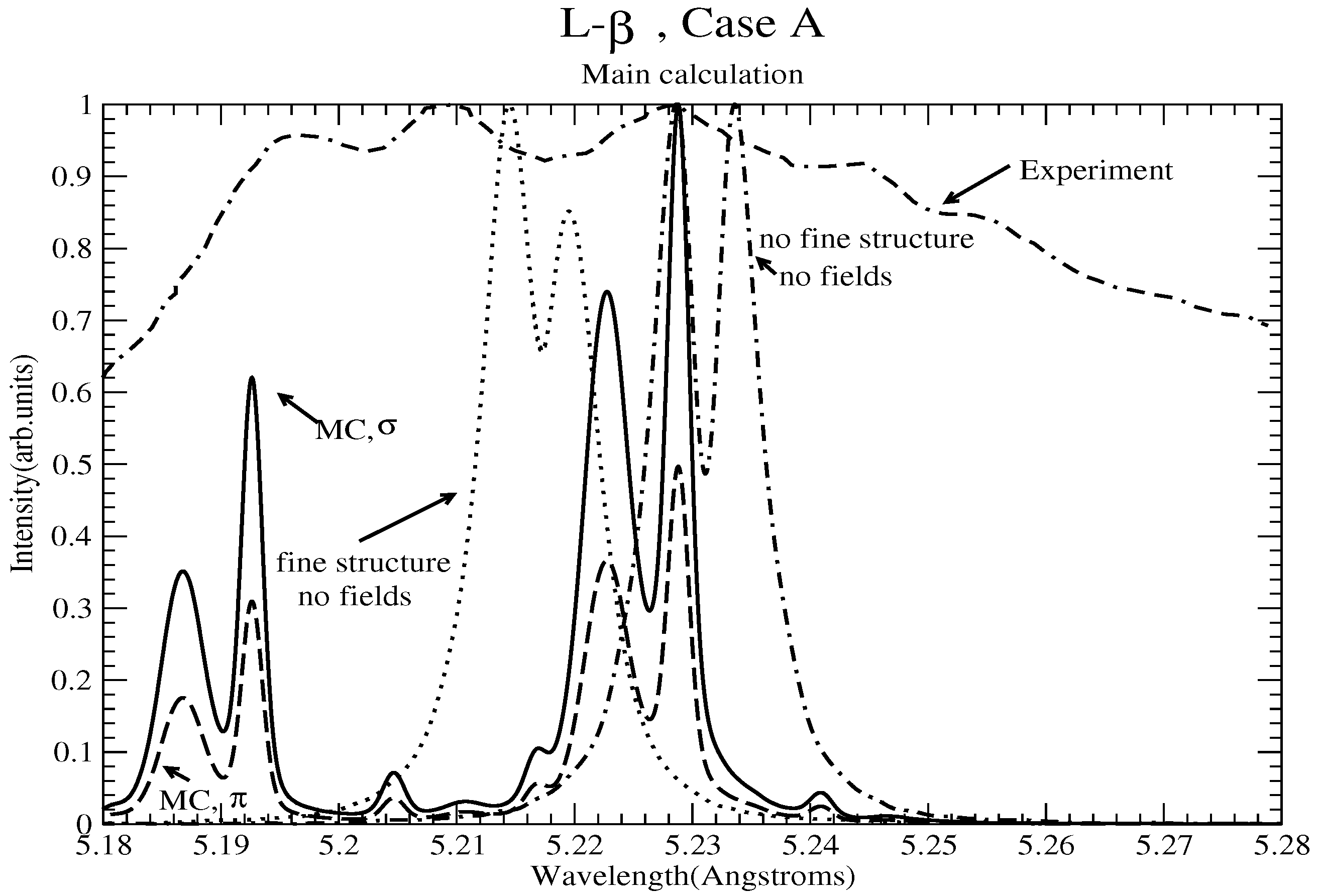
Figure 1.
Main calculation for
, case A. Shown are the
(solid line) and
(dashed line) profiles for the main calculation; the profiles for the calculations without oscillatory and static fields, with (dotted line) and without (dashed−dotted line) fine structure; and the experimental profile (dot−double−dashed line) of Ref. [
10].
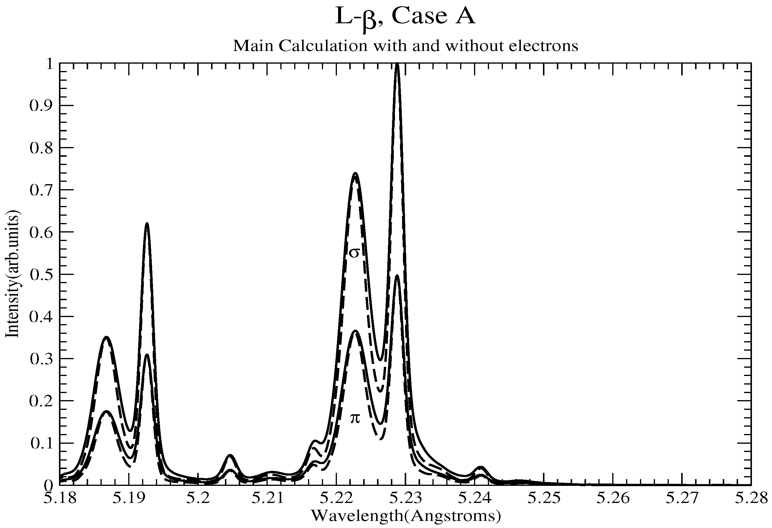
Figure 2.
Main calculation for , case A, with only ion broadening accounted for (i.e., no electrons). Shown are the main calculation and profiles (solid line), along with the corresponding profiles for the calculations without electron broadening (dashed line).
Figure 2.
Main calculation for , case A, with only ion broadening accounted for (i.e., no electrons). Shown are the main calculation and profiles (solid line), along with the corresponding profiles for the calculations without electron broadening (dashed line).
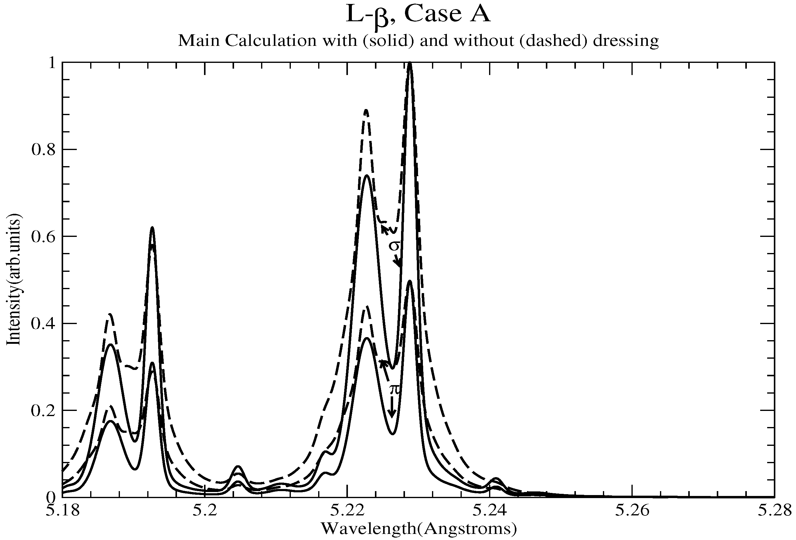
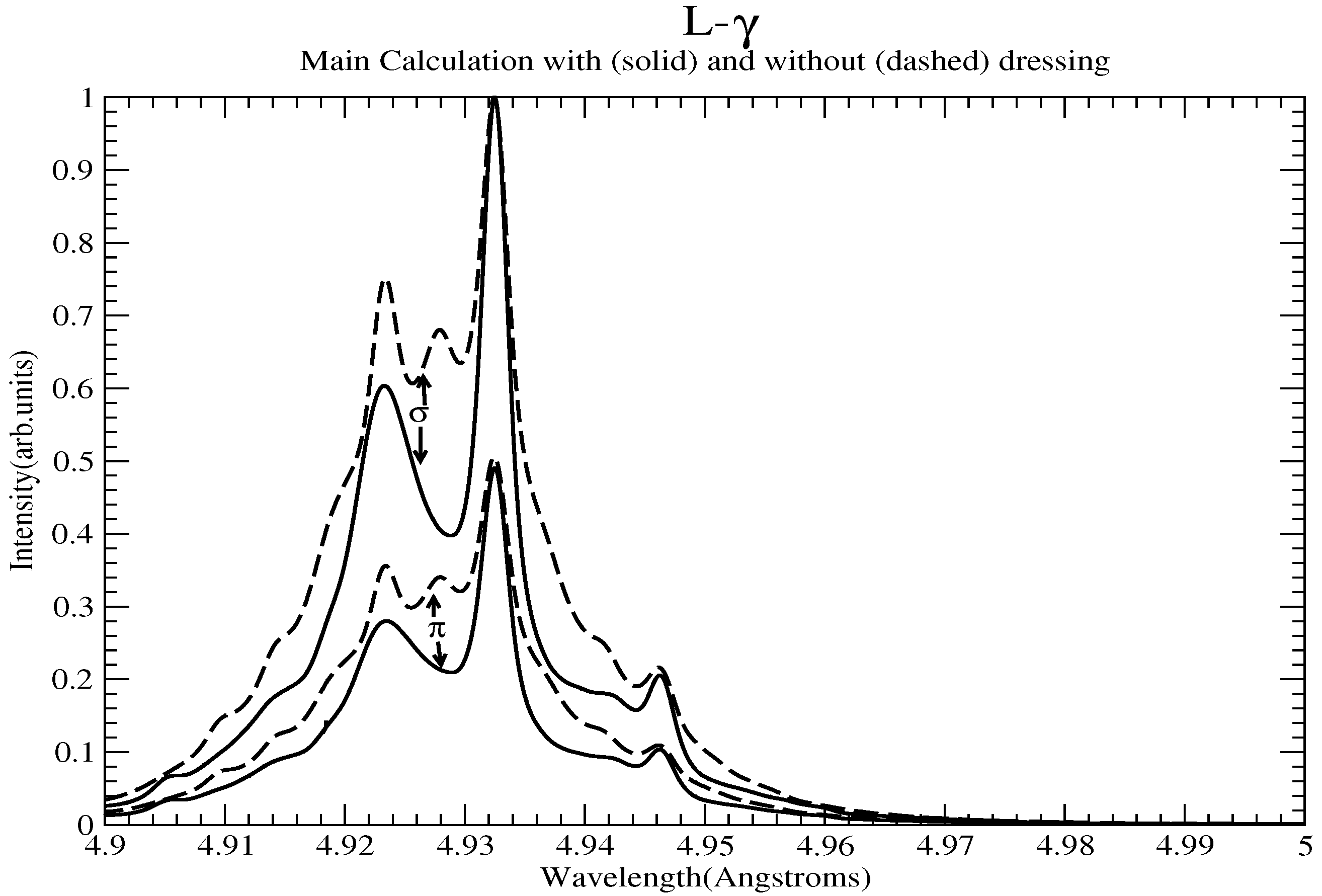
Figure 3.
Effect of dressing for , case A. Shown are and profiles for the main calculation (solid line) and the “no dressing” calculation (dashed line); i.e., the matrix S which described the satellite positions and intensities was correctly computed, but the emitter–plasma interaction was (incorrectly) not dressed by the nonrandom static and oscillatory fields.
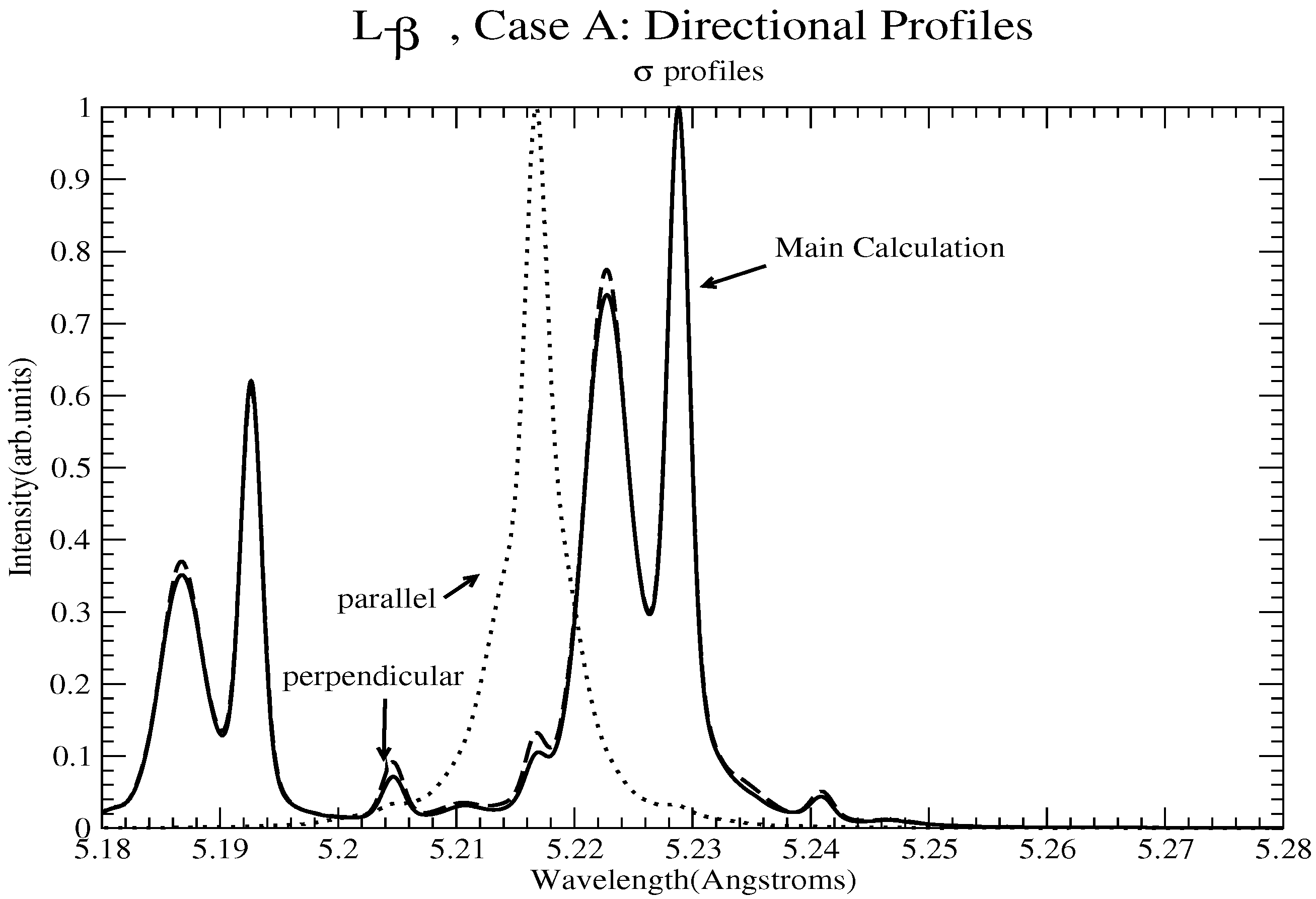
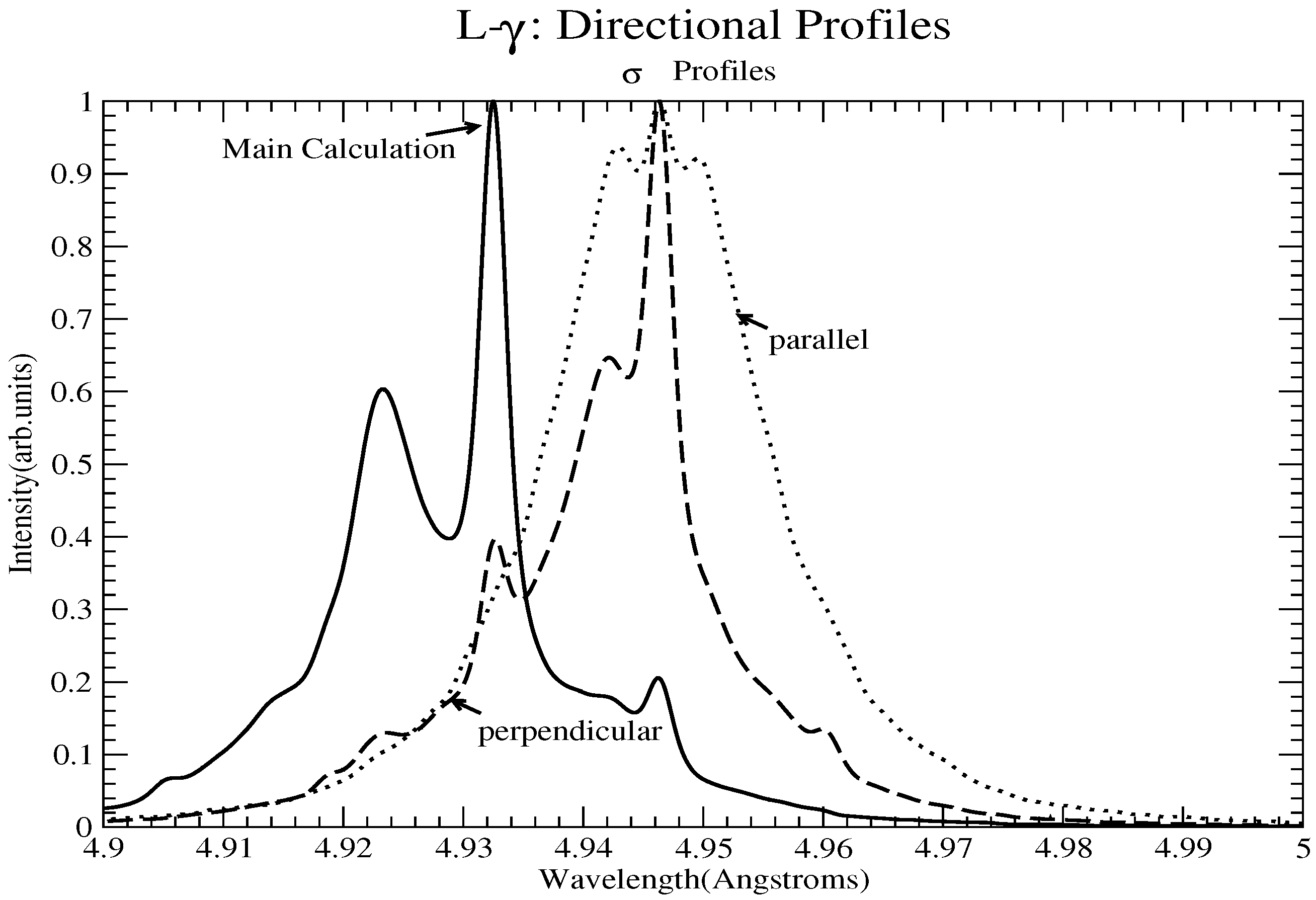
Figure 4.
Directional effects for , case A. Shown are profiles for the main calculation (solid line) and the entire static field (4.8 GV/cm) when parallel (dotted line) or perpendicular (dashed line) to the oscillatory field.
Figure 4.
Directional effects for , case A. Shown are profiles for the main calculation (solid line) and the entire static field (4.8 GV/cm) when parallel (dotted line) or perpendicular (dashed line) to the oscillatory field.
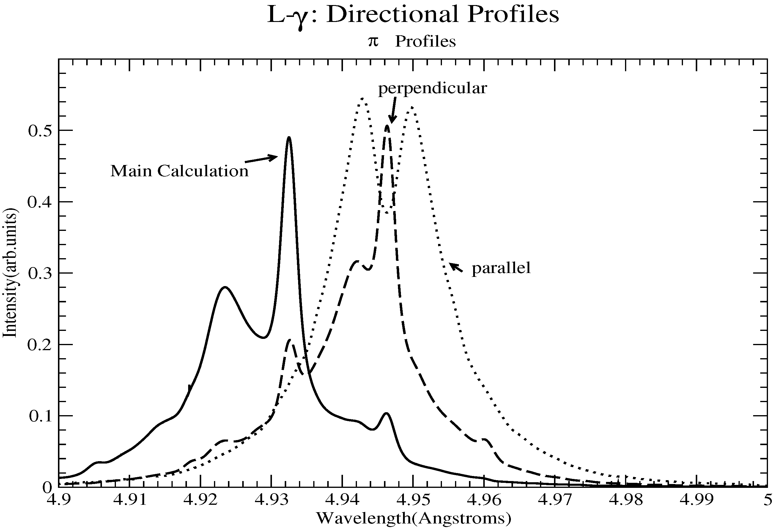
Figure 5.
Directional effects for , case A. Shown are profiles for the main calculation (solid line) and the entire static field (4.8 GV/cm) when parallel (dotted line) or perpendicular (dashed line) to the oscillatory field.
Figure 5.
Directional effects for , case A. Shown are profiles for the main calculation (solid line) and the entire static field (4.8 GV/cm) when parallel (dotted line) or perpendicular (dashed line) to the oscillatory field.
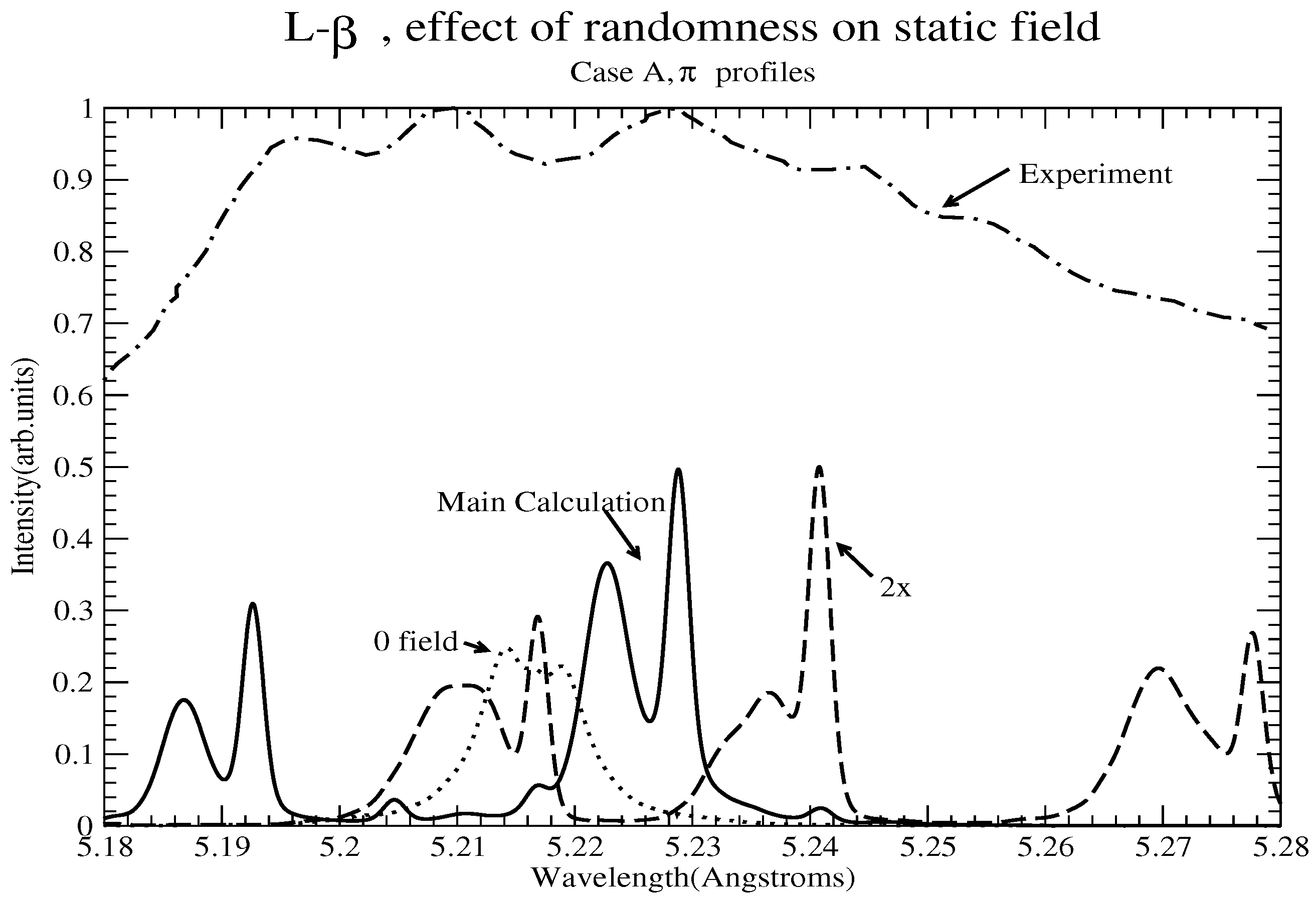
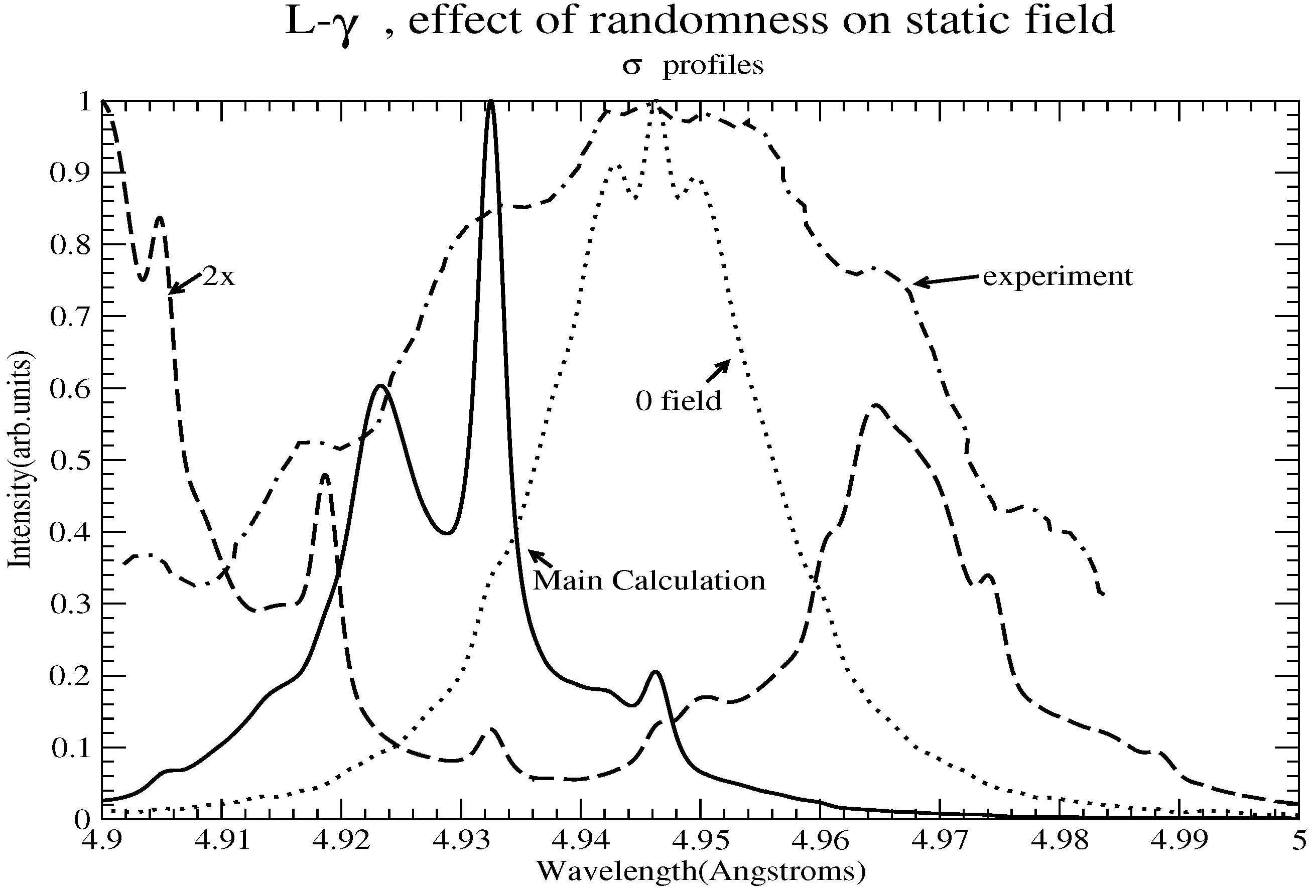
Figure 6.
Randomness of static component perpendicular to the oscillatory field for , case A. Shown are profiles for the main calculation (solid line), the component perpendicular to oscillatory field 0 (0 field-dotted) and the component perpendicular to the oscillatory field but twice the size of that in the main calculation, i.e., 8.24 GV/cm (2x-dashed). The static component perpendicular to the oscillatory field is the same as in the main calculation, 2.46 GV/cm. Shown as well is the experimental profile (dashed–dotted line).
Figure 7.
Randomness of static component perpendicular to the oscillatory field for , case A. Shown are profiles for the main calculation (solid line), the component perpendicular to oscillatory field 0 (0 field-dotted) and the component perpendicular to the oscillatory field but twice the size of that in the main calculation, i.e., 8.24 GV/cm (2x-dashed). The static component perpendicular to the oscillatory field is the same as in the main calculation, 2.46 GV/cm. Shown as well is the experimental profile (dashed–dotted line).
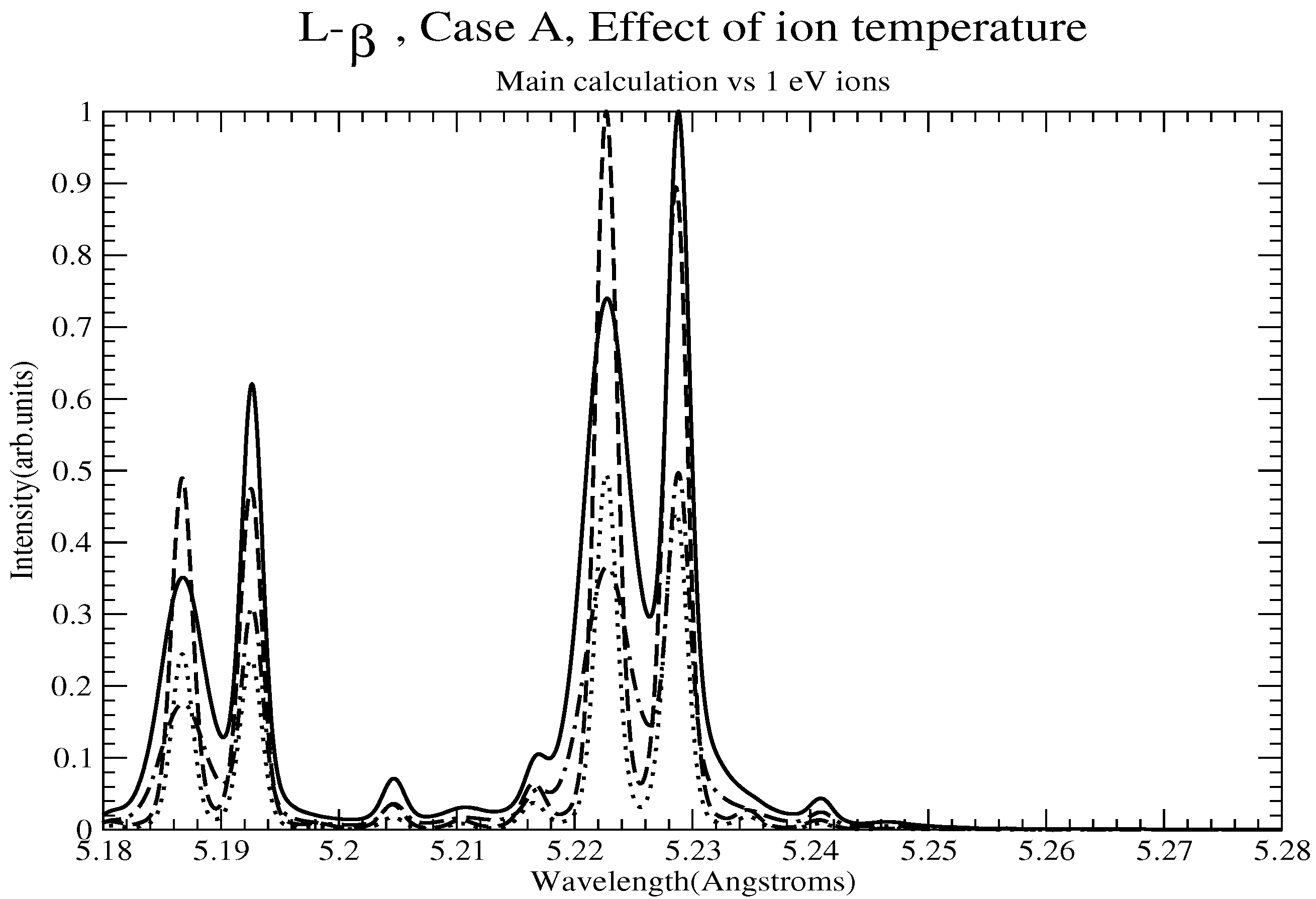
Figure 8.
(solid line) and (dashed–dotted line) main calculation profiles, and the corresponding (dashed line) and (dotted line) profiles for an ion temperature of 1 eV.
Figure 8.
(solid line) and (dashed–dotted line) main calculation profiles, and the corresponding (dashed line) and (dotted line) profiles for an ion temperature of 1 eV.
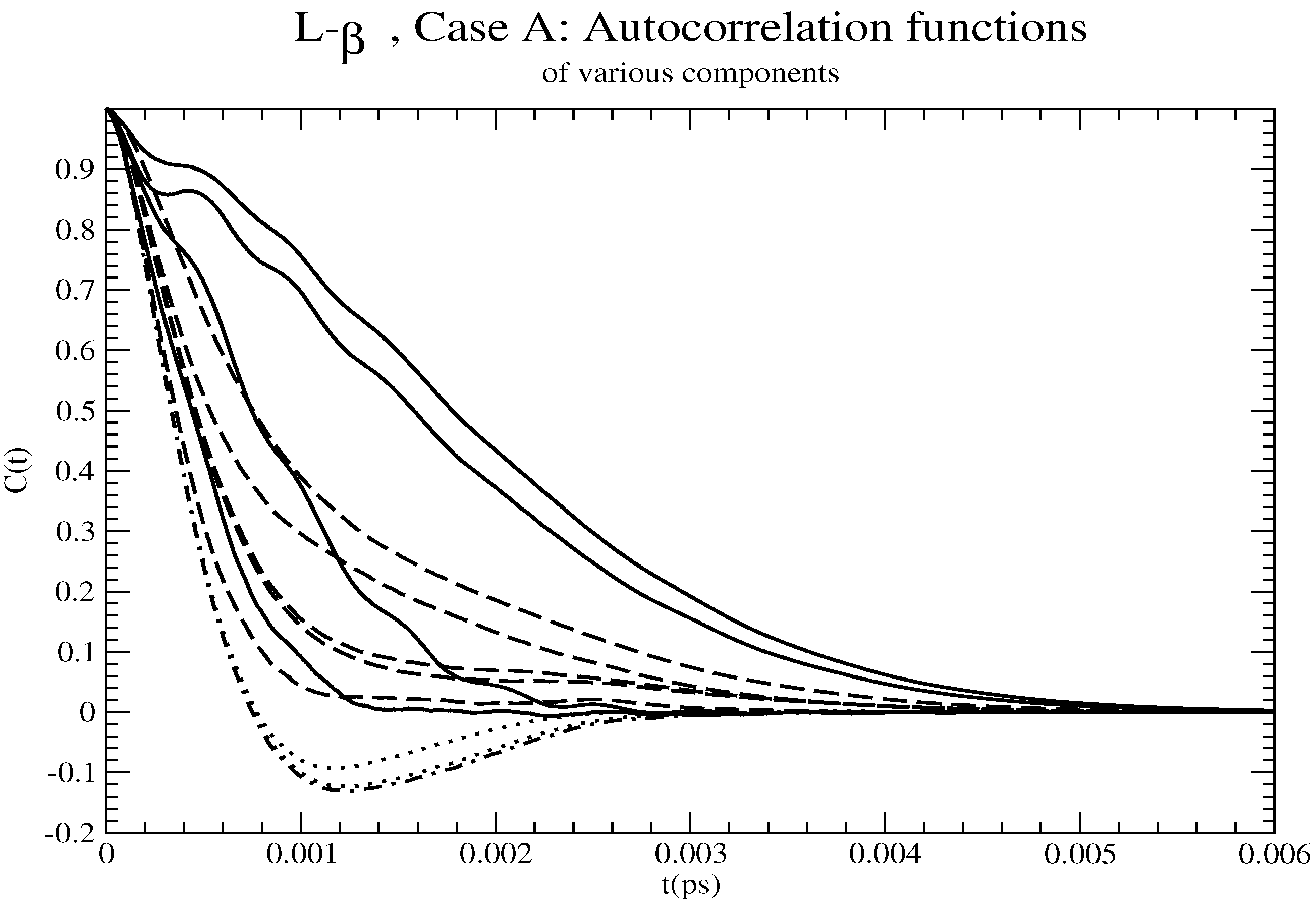
Figure 9.
Autocorrelation functions C(t) for the various components (corresponding to different Blokhintsev–Floquet peaks) of the , case A calculation. The solid lines correspond to the “main calculation” components; the dotted lines correspond to the two finely structured components in the absence of oscillatory and static fields. The dashed–dotted line corresponds to the calculation without fine structure and without oscillatory or static fields. The dashed lines are the components in the calculation where dressing was turned off.
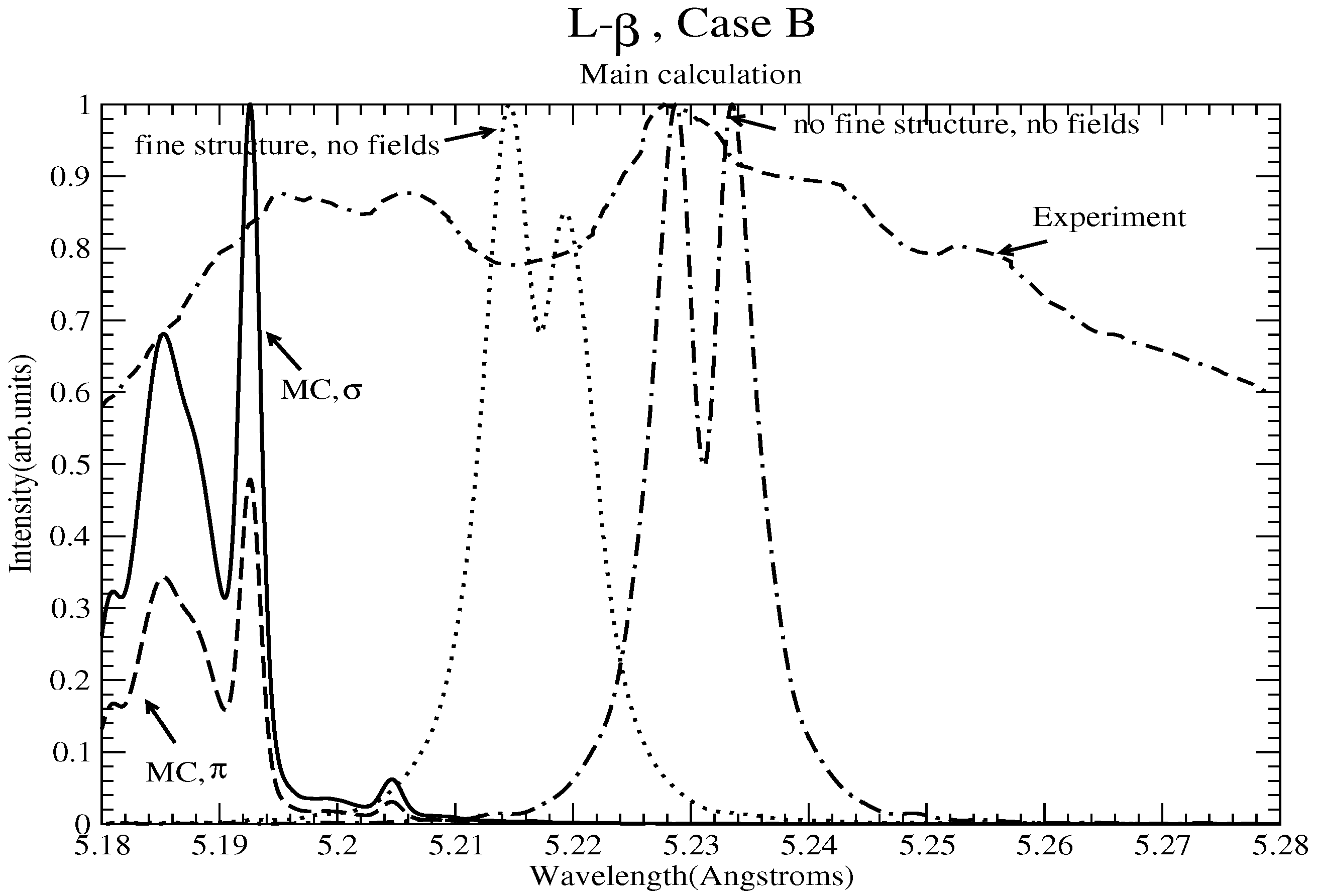
Figure 10.
Main calculation for
, case B. Shown are the
(solid line) and
(dashed line) profiles for the main calculation; the profile without oscillatory and static fields, with (dotted line) and without (dashed–dotted line) fine structure; and the experimental profile (dot–double-dashed line) of Ref. [
10].
Figure 11.
Positions and intensities for the main calculation for , cases A(+) and B(*). is measured from the line center of gravity.
Figure 11.
Positions and intensities for the main calculation for , cases A(+) and B(*). is measured from the line center of gravity.
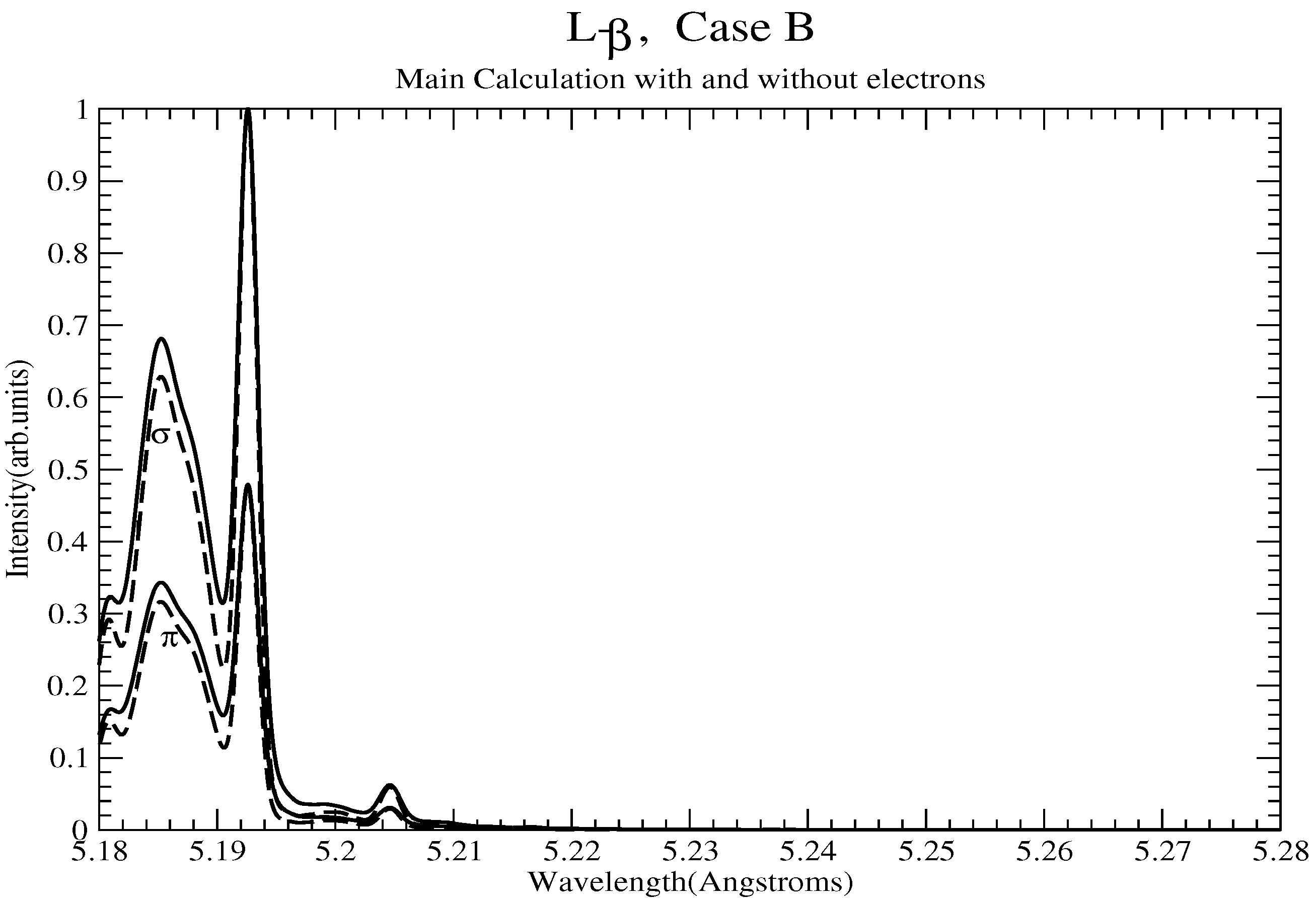
Figure 12.
Main Calculation for , case B with only ion broadening accounted for (i.e., no electrons). Shown are the main calculation and profiles (solid line), together with the profiles for the calculations without electron broadening (dashed line).
Figure 12.
Main Calculation for , case B with only ion broadening accounted for (i.e., no electrons). Shown are the main calculation and profiles (solid line), together with the profiles for the calculations without electron broadening (dashed line).
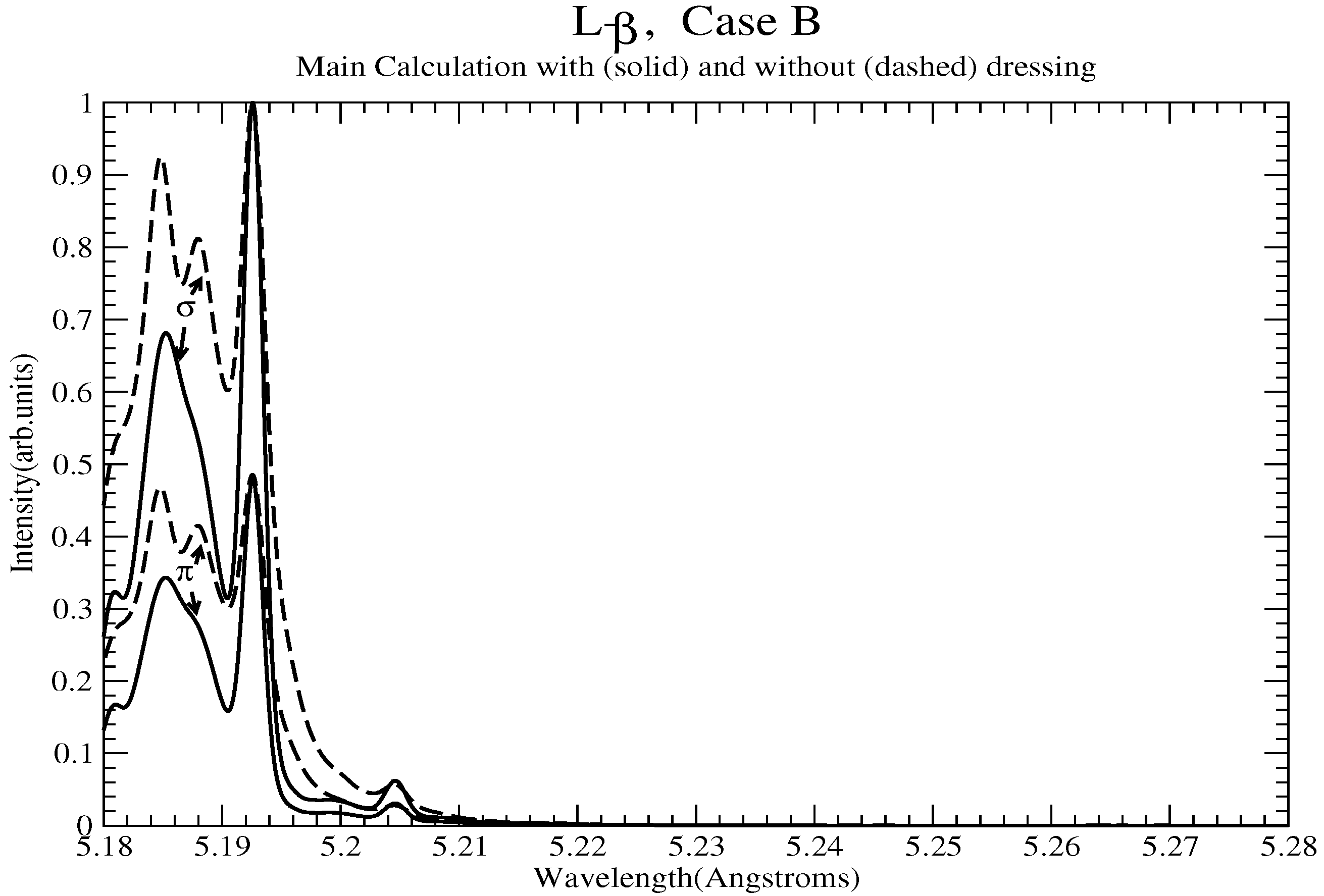
Figure 13.
Effect of dressing for , case B. Shown are and profiles for the main calculation (solid line) and the “no dressing” calculation (dashed line), i.e., the matrix S, which described the satellite positions and intensities, was correctly computed, but the emitter–plasma interaction was (incorrectly) not dressed by the nonrandom static and oscillatory fields.
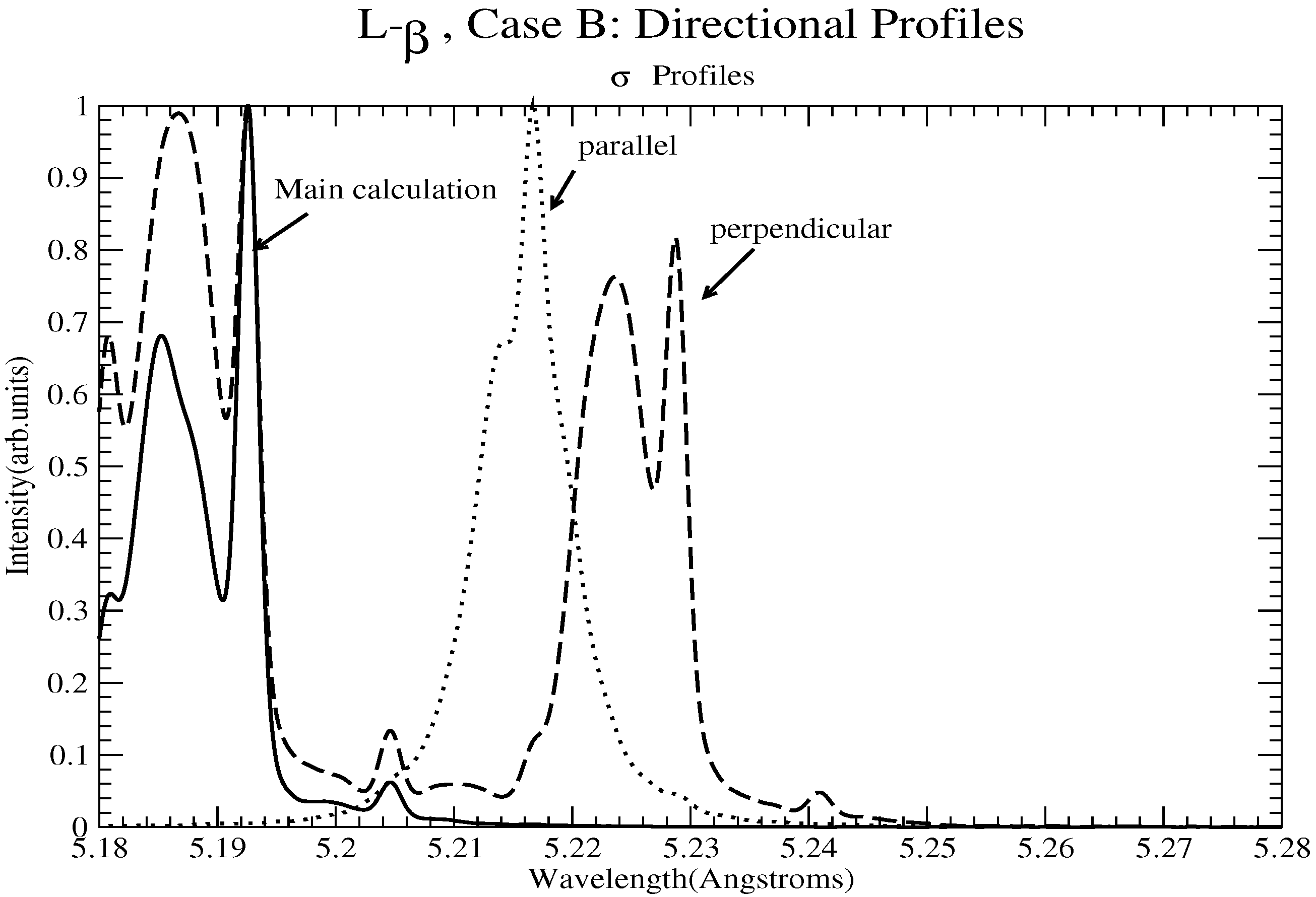
Figure 14.
Directional effects for , case B. Shown are profiles for the main calculation (solid line) and the entire static field (4.4 GV/cm) when parallel (dotted line) or perpendicular (dashed line) to the oscillatory field.
Figure 14.
Directional effects for , case B. Shown are profiles for the main calculation (solid line) and the entire static field (4.4 GV/cm) when parallel (dotted line) or perpendicular (dashed line) to the oscillatory field.
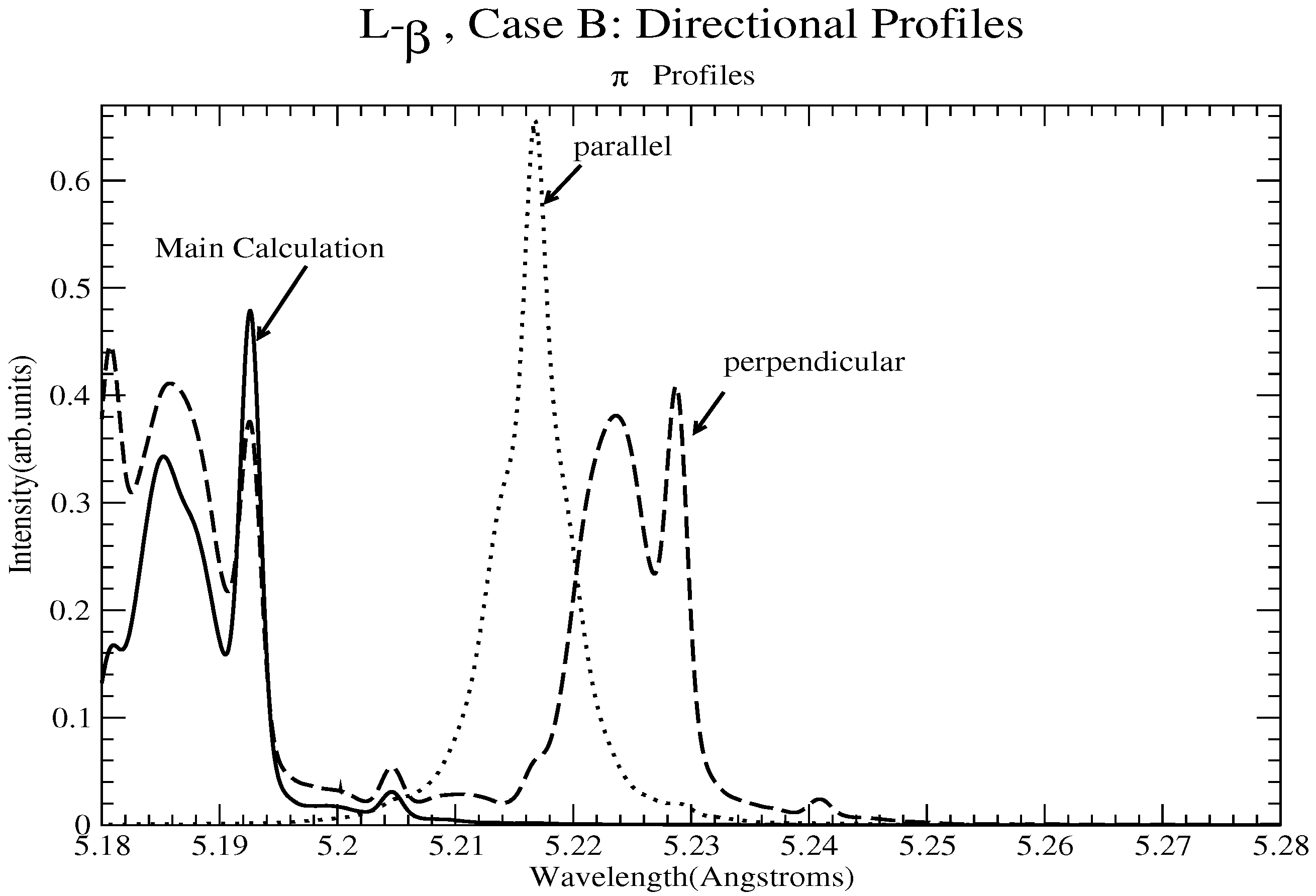
Figure 15.
Directional Effects for , case B. Shown are profiles for the main calculation (solid line) and the entire static field (4.4 GV/cm) when parallel (dotted line) or perpendicular (dashed line) to the oscillatory field.
Figure 15.
Directional Effects for , case B. Shown are profiles for the main calculation (solid line) and the entire static field (4.4 GV/cm) when parallel (dotted line) or perpendicular (dashed line) to the oscillatory field.
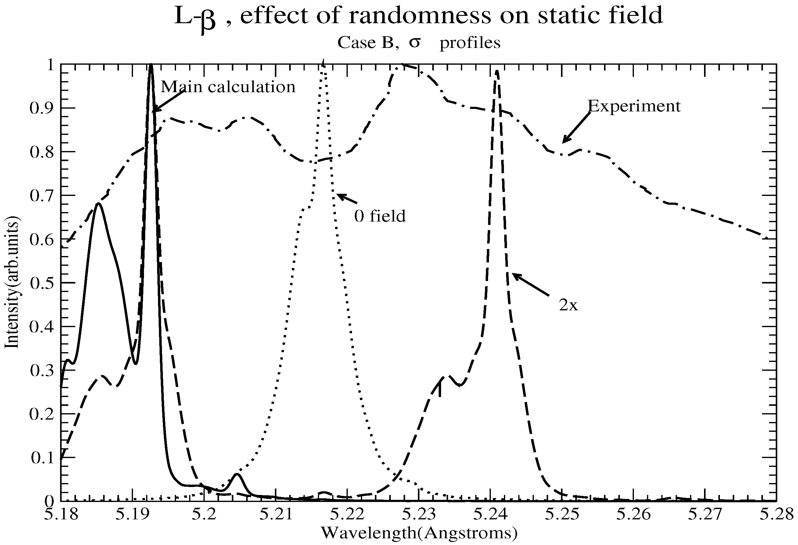
Figure 16.
Randomness of static component perpendicular to the oscillatory field for , case B. Shown are profiles for the main calculation (solid line), the component perpendicular to oscillatory field 0 (0 field-dotted) and the component perpendicular to the oscillatory field but twice the size of that in the main calculation, i.e., 6.44 GV/cm (2x-dashed). The static component perpendicular to the oscillatory field is the same as in the main calculation, 3 GV/cm. Shown as well is the experimental profile (dashed–dotted line).
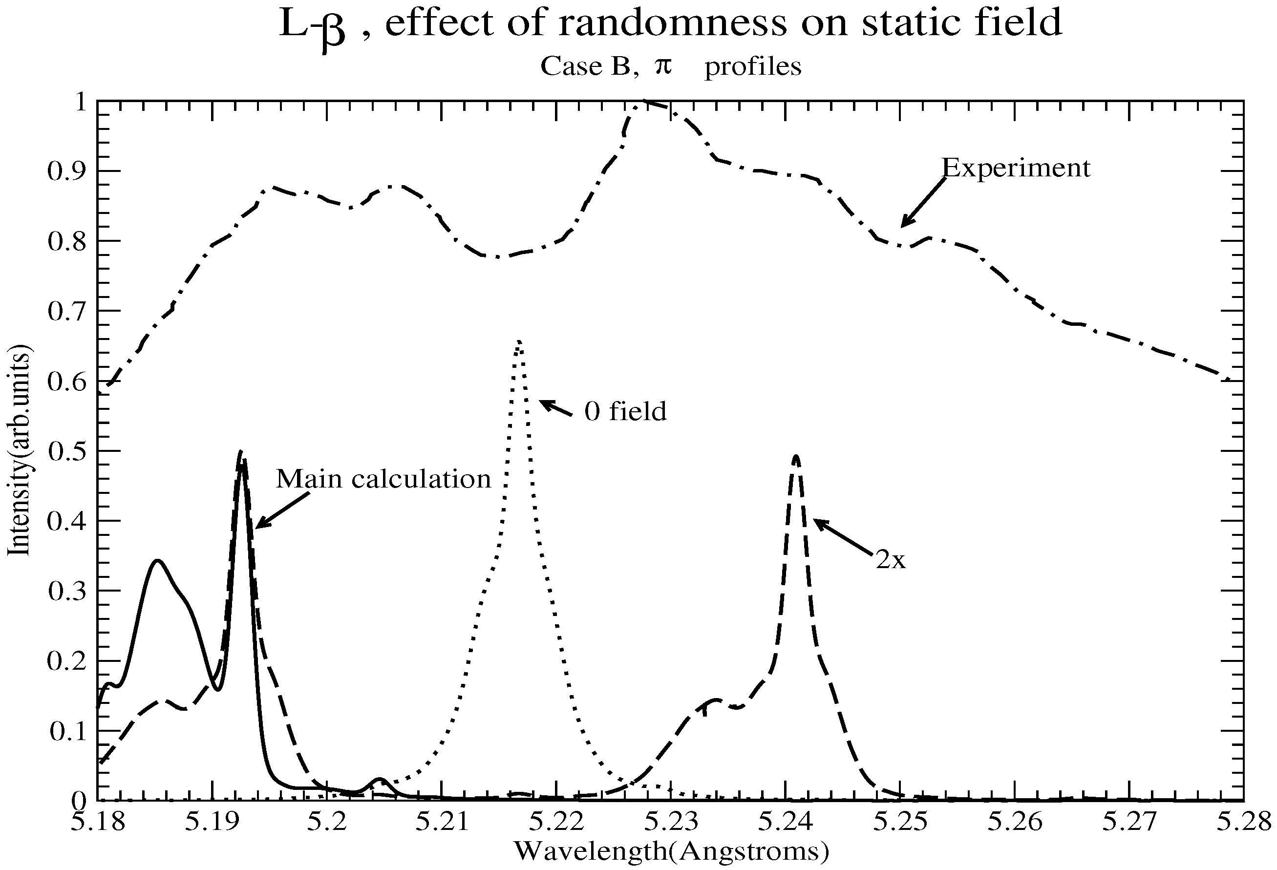
Figure 17.
Randomness of static component perpendicular to the oscillatory field for , case B. Shown are profiles for the main calculation (solid line), the component perpendicular to oscillatory field 0 (0 field-dotted) and the component perpendicular to the oscillatory field but twice the size of that in the main calculation, i.e., 6.44 GV/cm (2x-dashed). The static component perpendicular to the oscillatory field is the same as in the main calculation, 3 GV/cm. Shown as well is the experimental profile (dashed–dotted line).
Figure 18.
(solid line) and (dashed–dotted line) main calculation profiles and the corresponding (dashed line) and (dotted line) profiles for an ion temperature of 1 eV.
Figure 18.
(solid line) and (dashed–dotted line) main calculation profiles and the corresponding (dashed line) and (dotted line) profiles for an ion temperature of 1 eV.
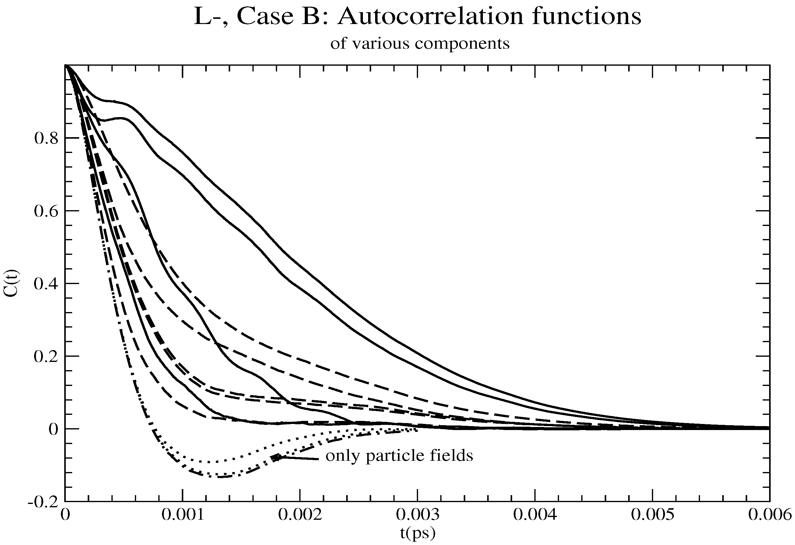
Figure 19.
Autocorrelation functions C(t) for the various components (corresponding to different Blokhintsev–Floquet peaks) of the , case B calculation. The solid lines correspond to the “main calculation” components; the dotted lines correspond to the two finely structured components in the absence of oscillatory and static fields. The dashed−dotted line corresponds to the calculation without fine structure and without oscillatory or static fields. The dashed lines are the components in the calculation where dressing was turned off.
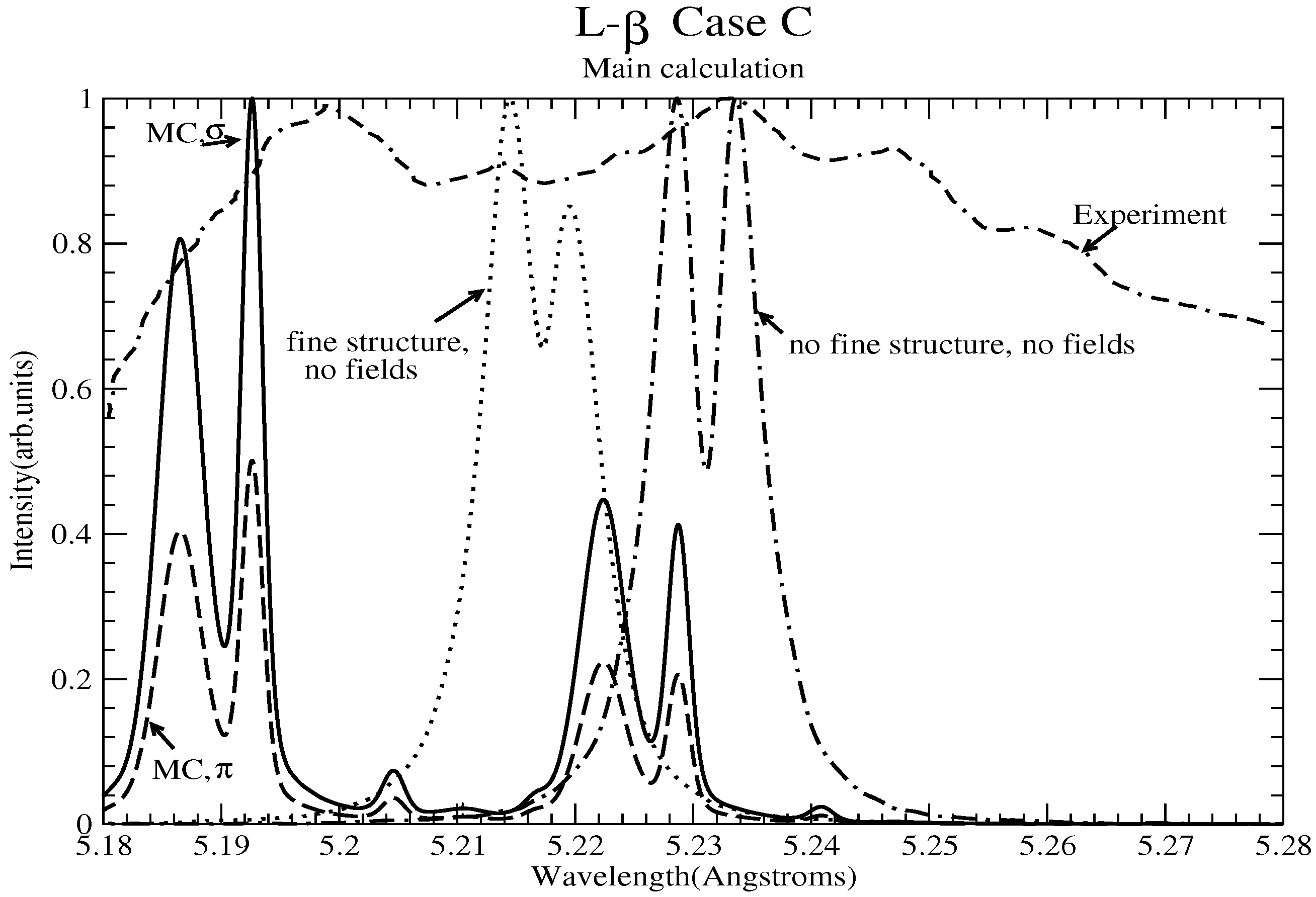
Figure 20.
Main calculation for
, case C. Shown are the
(solid line) and
(dashed line) profiles for the main calculation; the profiles for the calculations without an oscillatory or a static field with (dotted line) or without (dashed−dotted line) fine structure; and the experimental profile (dot−double−dashed line) of [
9,
10].
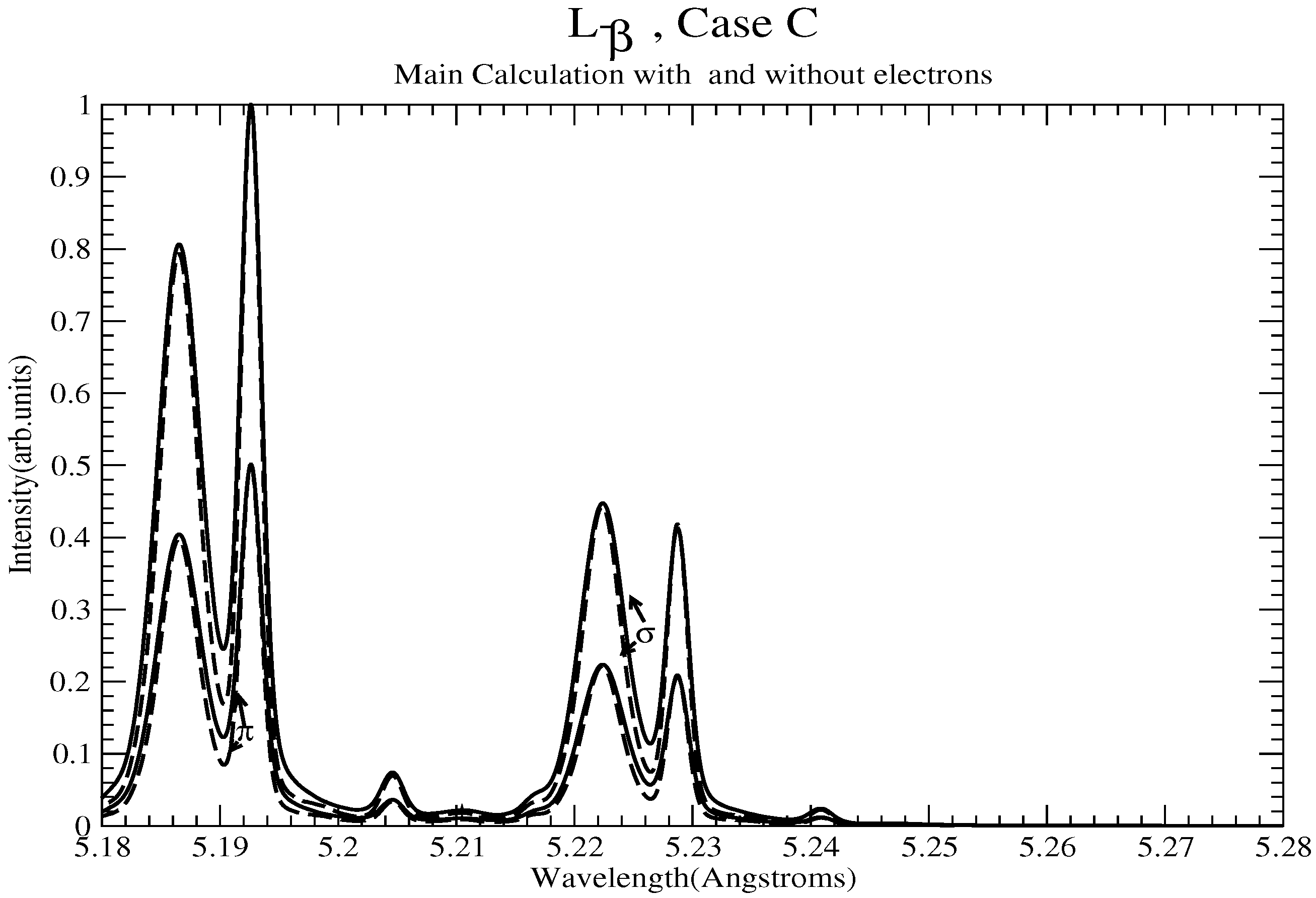
Figure 21.
Main calculation for , case C with only ion broadening accounted for (i.e., no electrons). Shown are the main calculation’s and profiles (solid line), along with the profiles for the calculations without electron broadening (dashed for the and dash−dot for the profile).
Figure 21.
Main calculation for , case C with only ion broadening accounted for (i.e., no electrons). Shown are the main calculation’s and profiles (solid line), along with the profiles for the calculations without electron broadening (dashed for the and dash−dot for the profile).
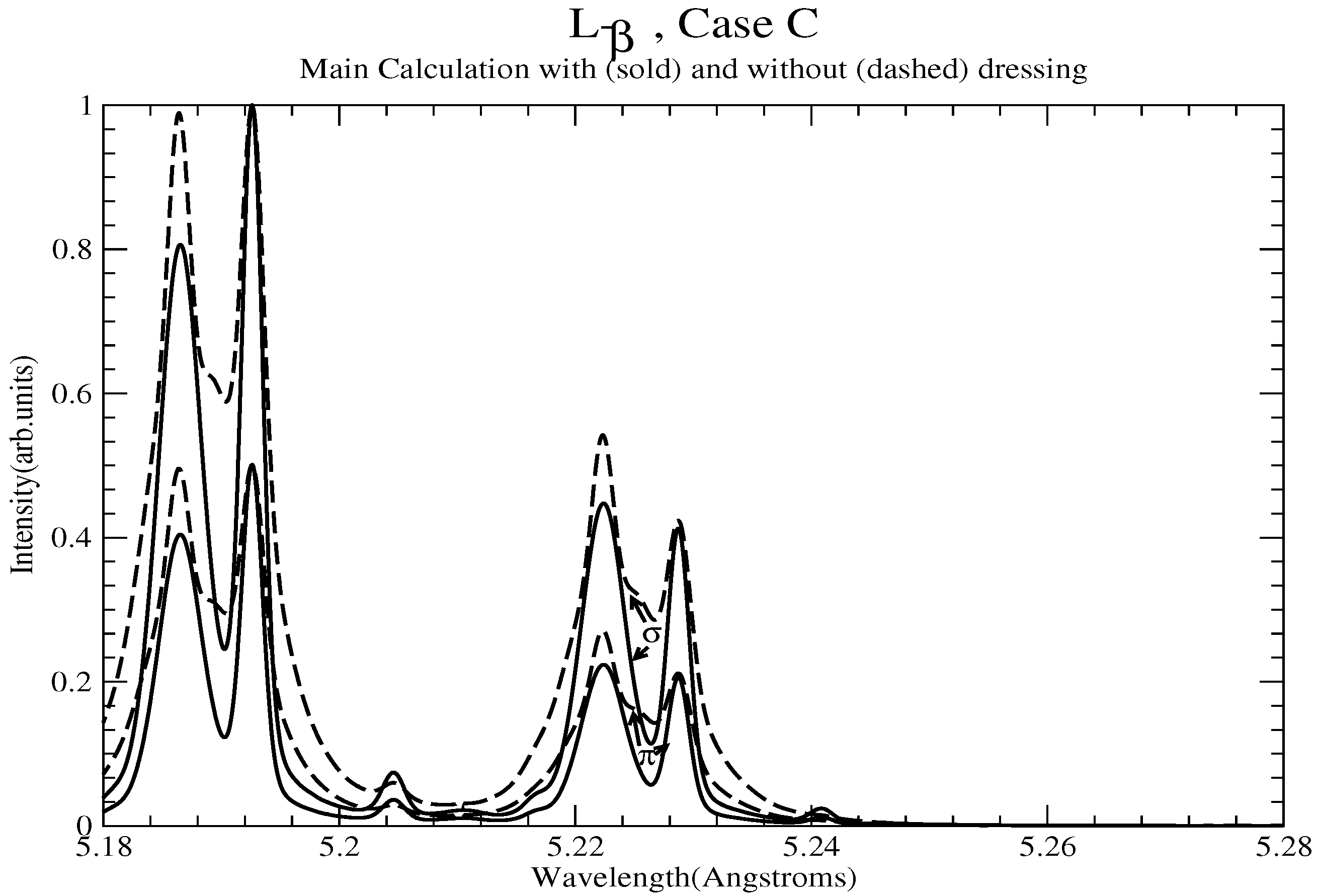
Figure 22.
Effect of Dressing for , case C. Shown are and profiles for the main calculation (solid line) and the “no dressing” calculation (dashed line), i.e., the matrix S which described the satellite positions and intensities is correctly computed, but the emitter–plasma interaction is (incorrectly) not dressed by the nonrandom static and oscillatory fields.
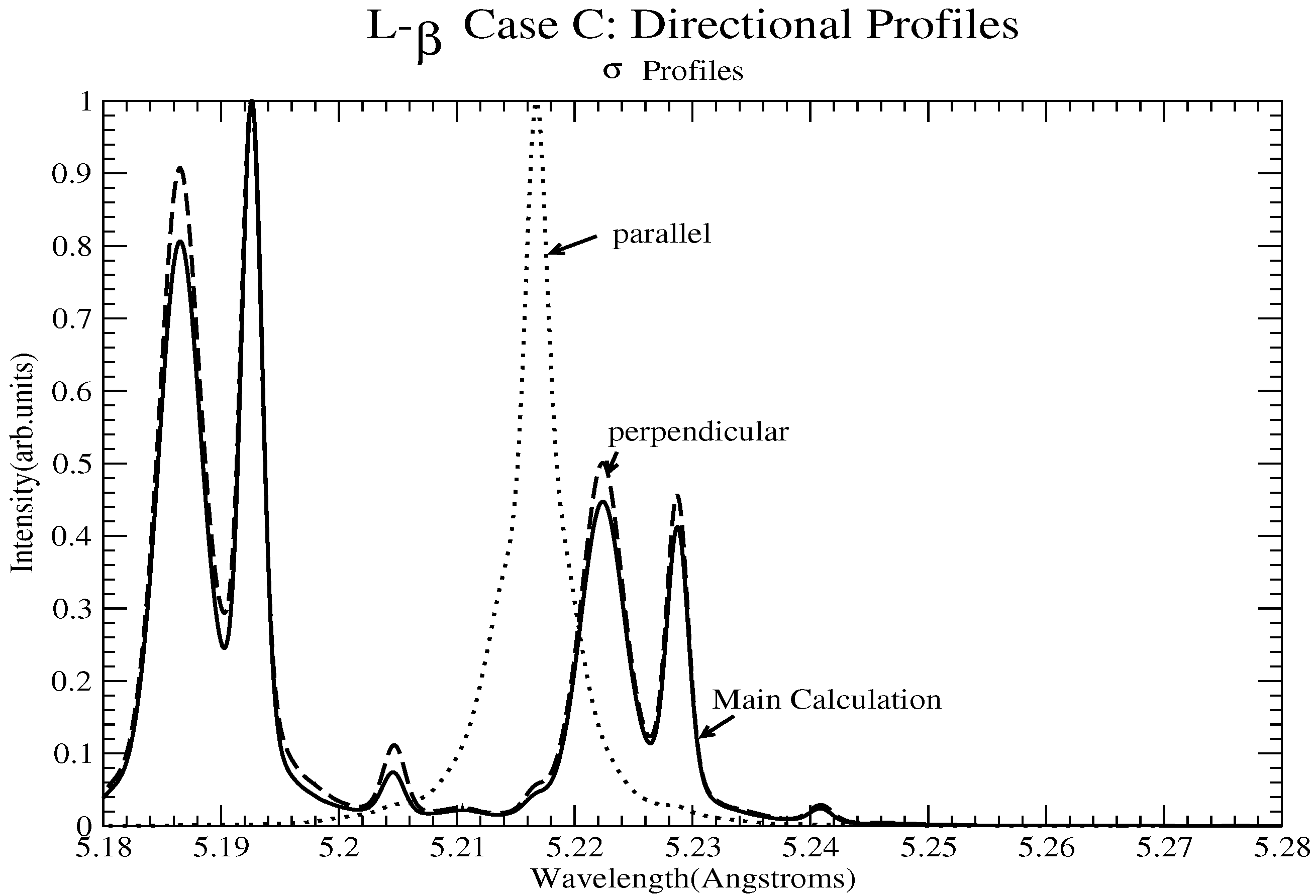
Figure 23.
Directional Effects for , case C. Shown are profiles for the main calculation (solid line), and with the entire static field (4.9 GV/cm) when parallel (dotted line) or perpendicular (dashed line) to the oscillatory field.
Figure 23.
Directional Effects for , case C. Shown are profiles for the main calculation (solid line), and with the entire static field (4.9 GV/cm) when parallel (dotted line) or perpendicular (dashed line) to the oscillatory field.
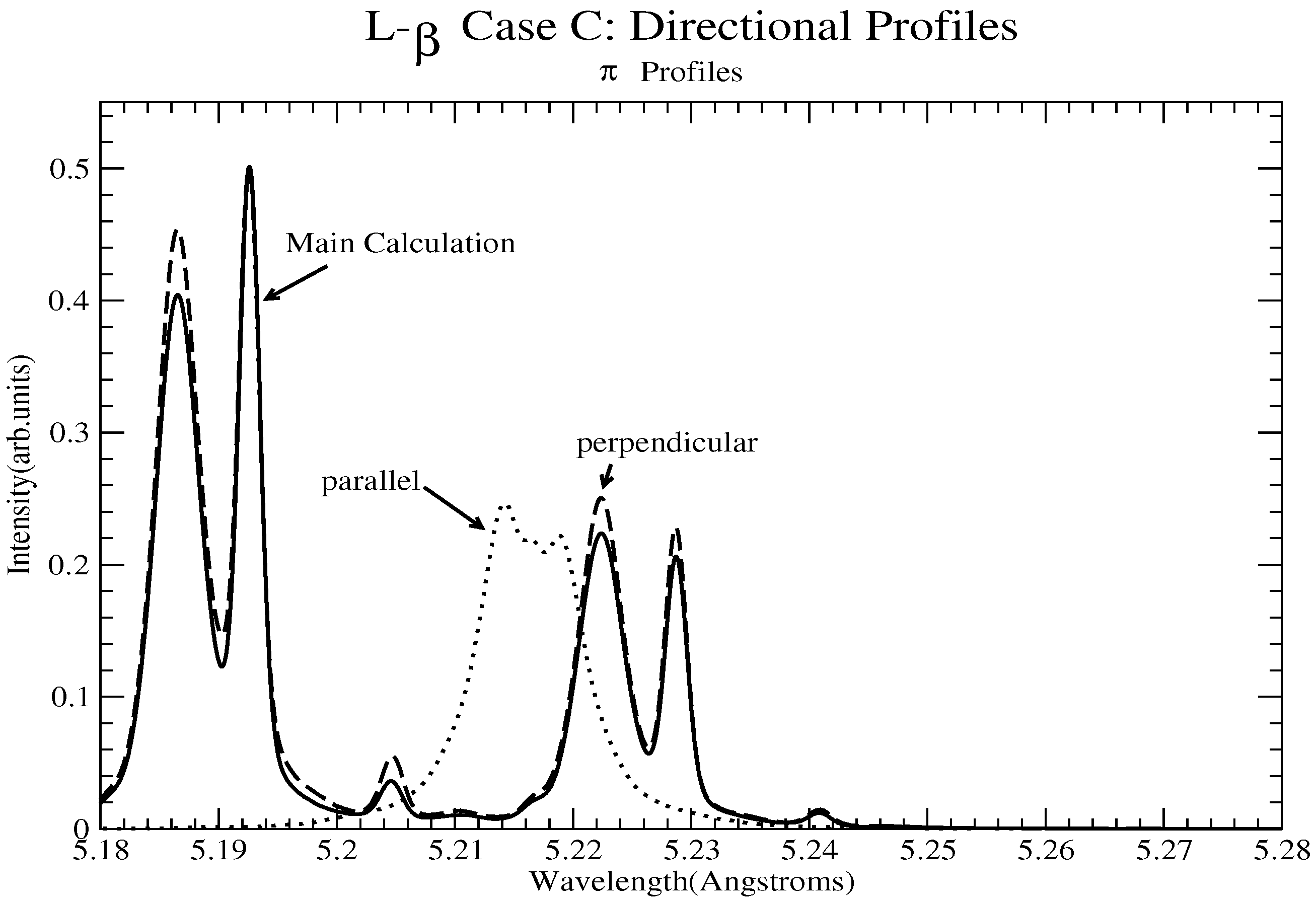
Figure 24.
Directional effects for , case C. Shown are profiles for the main calculation (solid line) and the entire static field (4.9 GV/cm) when parallel (dotted line) or perpendicular (dashed line) to the oscillatory field.
Figure 24.
Directional effects for , case C. Shown are profiles for the main calculation (solid line) and the entire static field (4.9 GV/cm) when parallel (dotted line) or perpendicular (dashed line) to the oscillatory field.
Figure 25.
Randomness of the static component perpendicular to the oscillatory field for , case C. Shown are profiles for the main calculation (solid line), the component perpendicular to oscillatory field 0 (0 field-dotted) and the component perpendicular to the oscillatory field but twice the size of that in the main calculation, i.e., 7.74 GV/cm (2x-dashed). The static component perpendicular to the oscillatory field was the same as in the main calculation, 3 GV/cm. Shown as well is the experimental profile (dashe−dotted line).
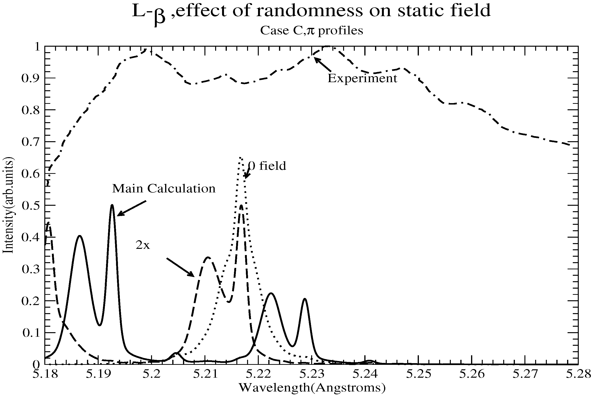
Figure 26.
Randomness of static component perpendicular to the oscillatory field for , case C. Shown are profiles for the main calculation (solid line), the component perpendicular to oscillatory field 0 (0 field-dotted) and the component perpendicular to the oscillatory field but twice the size of that in the main calculation, i.e., 7.74 GV/cm (2x-dashed). The static component perpendicular to the oscillatory field was the same as in the main calculation, 3 GV/cm. Shown as well is the experimental profile (dashed−dotted line).
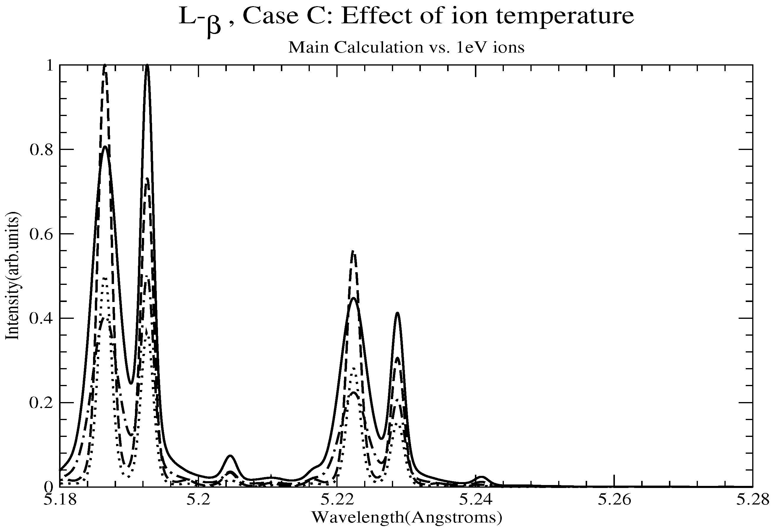
Figure 27.
(solid line) and (dashed–dotted line) main calculation profiles and the corresponding (dashed line) and (dotted line) profiles for an ion temperature of 1 eV.
Figure 27.
(solid line) and (dashed–dotted line) main calculation profiles and the corresponding (dashed line) and (dotted line) profiles for an ion temperature of 1 eV.
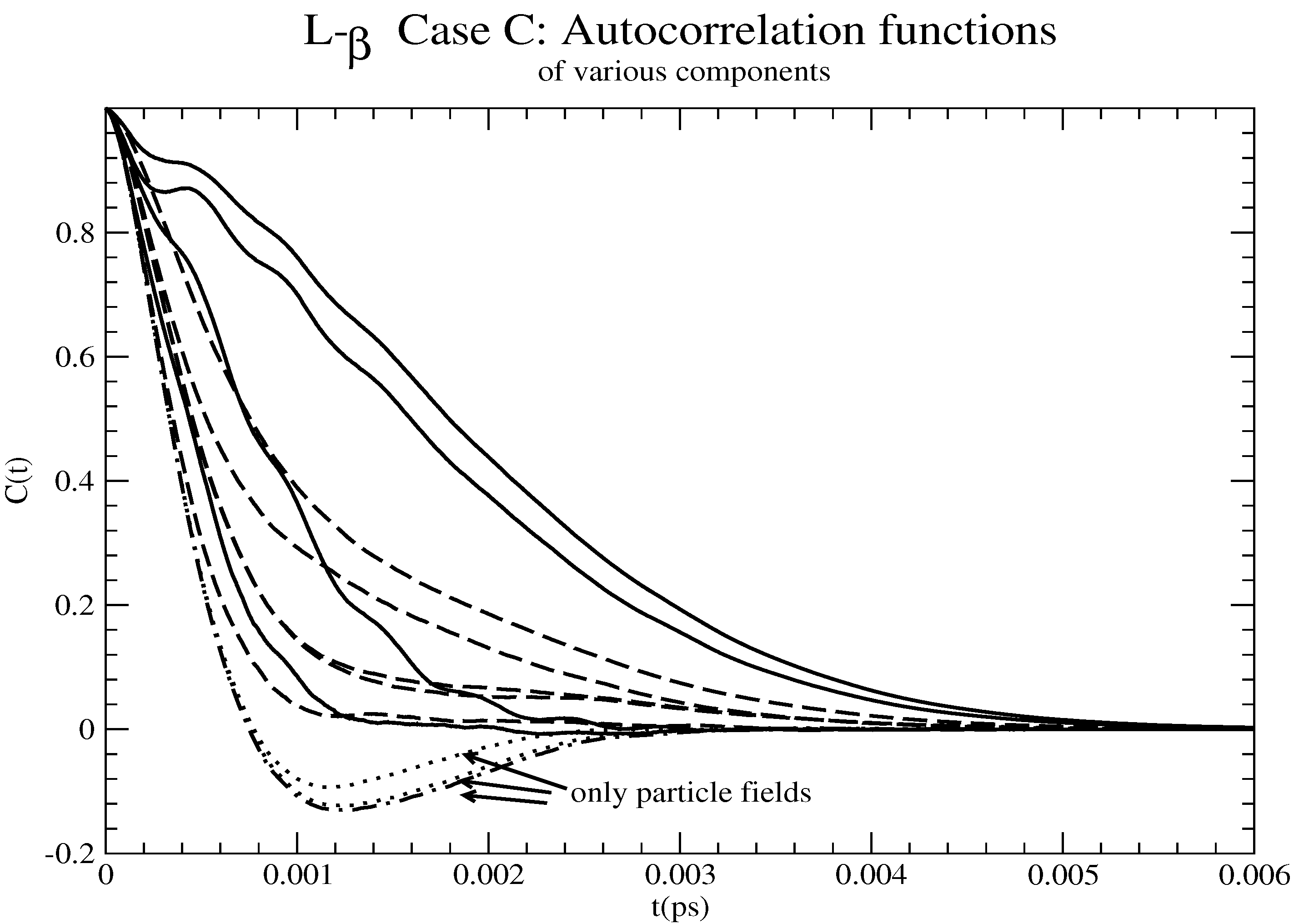
Figure 28.
Autocorrelation functions C(t) for the various components (corresponding to different Blokhintsev−Floquet peaks) of the , case C calculation. The solid lines correspond to the “main calculation” components; the dotted lines correspond to the two finely structured components in the absence of oscillatory and static fields. The dashed−dotted line corresponds to the calculation without fine structure and without oscillatory or static fields. The dashed lines are the components of the calculation where dressing was turned off.
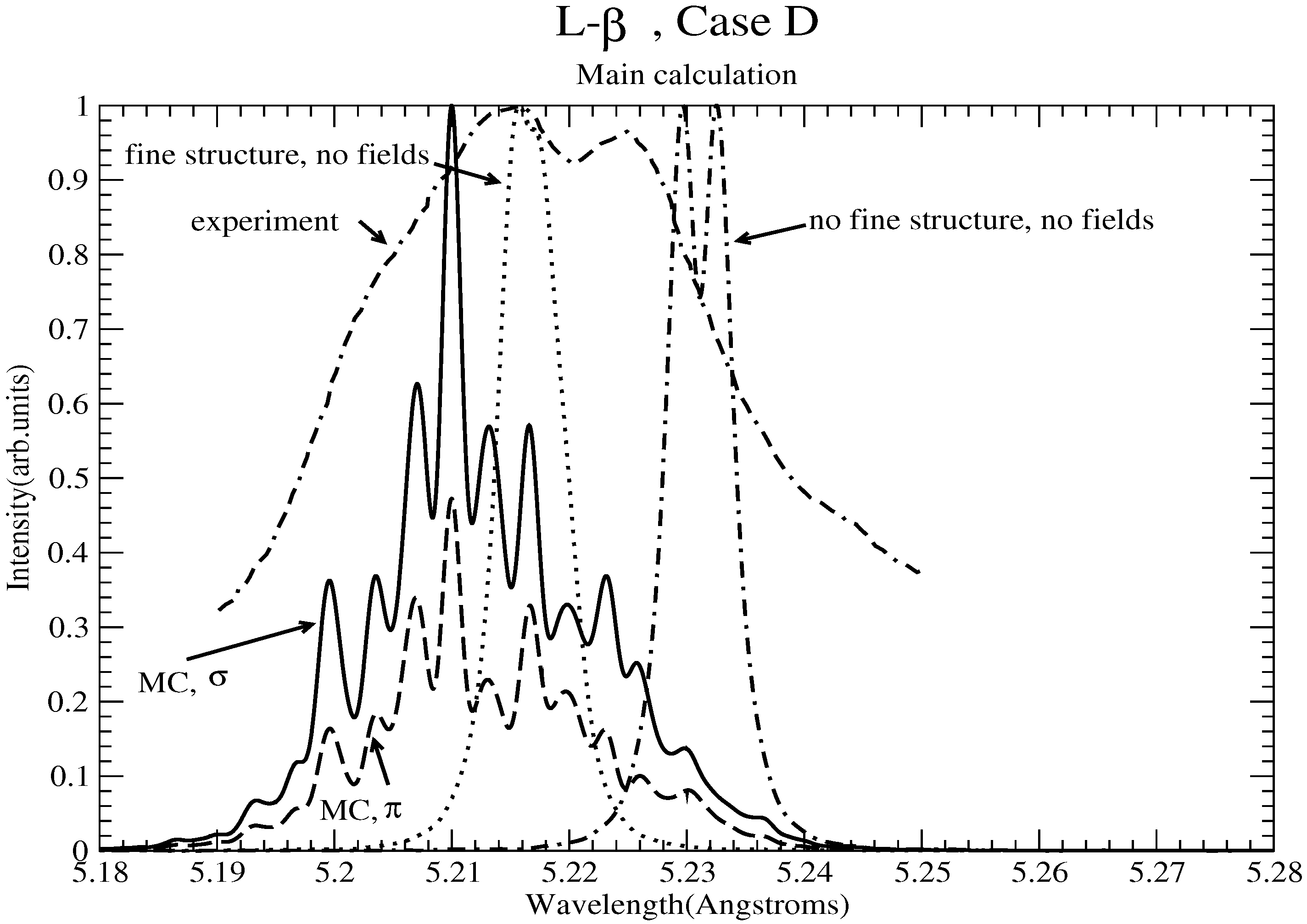
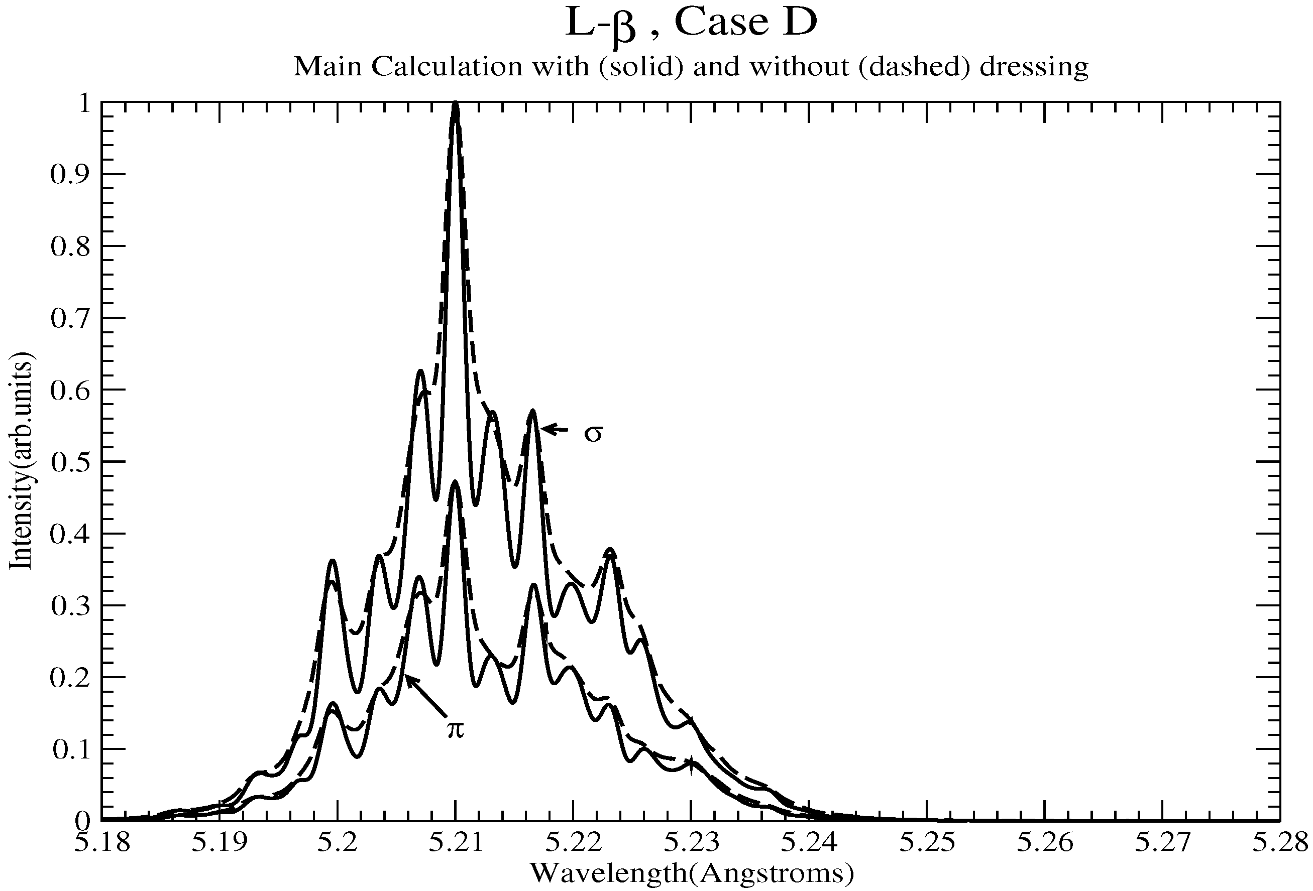
Figure 29.
Main calculation for
, case D. Shown are the
(solid line) and
(dashed line) profiles for the main calculation; the profiles for the calculations without an oscillatory or a static field, with (dotted line) and without (dashed–dotted line) fine structure; and the experimental profiles (dot–double-dashed line) of Refs. [
9,
10].
Figure 30.
Main calculation for , case D, with only ion broadening accounted for (i.e., no electrons). Shown are the main calculation’s and profiles (solid line), along with the profiles for the calculations without electron broadening (dashed for the and dash–dot for the profile).
Figure 30.
Main calculation for , case D, with only ion broadening accounted for (i.e., no electrons). Shown are the main calculation’s and profiles (solid line), along with the profiles for the calculations without electron broadening (dashed for the and dash–dot for the profile).
Figure 31.
Effect of dressing for , case D. Shown are and profiles for the main calculation (solid line) and the “no dressing” calculation (dashed line); i.e., the matrix S which described the satellite positions and intensities is correctly computed, but the emitter–plasma interaction is (incorrectly) not dressed by the nonrandom static and oscillatory fields.
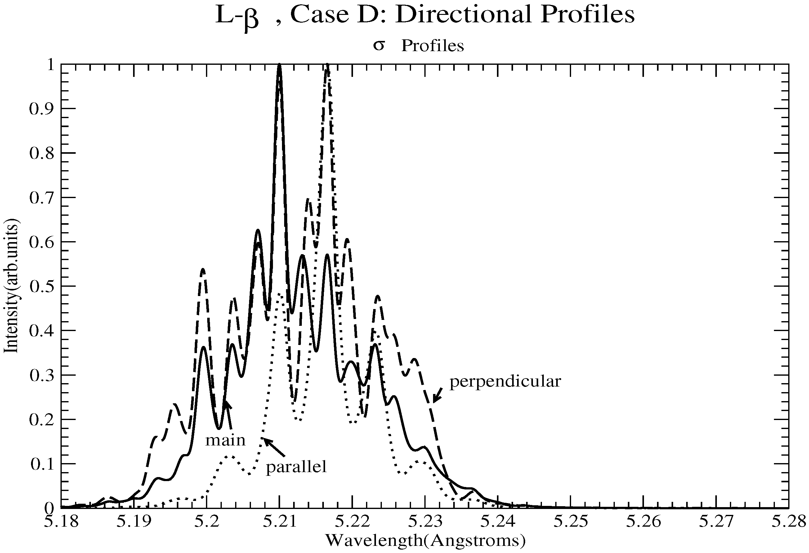
Figure 32.
Directional Effects for , case D. Shown are profiles for the main calculation (solid line) and the entire static field (2 GV/cm), parallel (dotted line) or perpendicular (dashed line) to the oscillatory field.
Figure 32.
Directional Effects for , case D. Shown are profiles for the main calculation (solid line) and the entire static field (2 GV/cm), parallel (dotted line) or perpendicular (dashed line) to the oscillatory field.
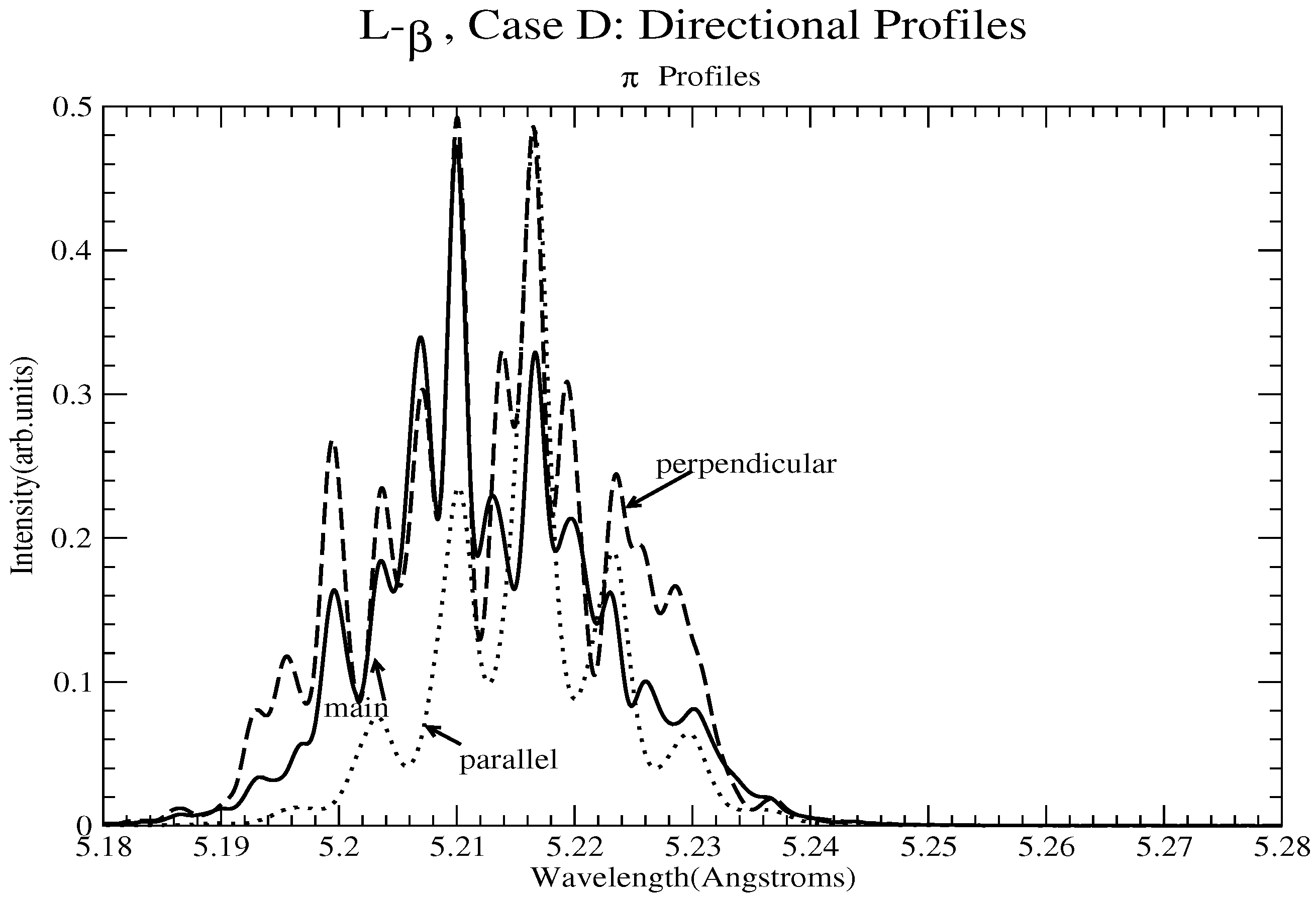
Figure 33.
Directional effects for , case D. Shown are profiles for the main calculation (solid line) and the entire static field (2 GV/cm) when parallel (dotted line) or perpendicular (dashed line) to the oscillatory field.
Figure 33.
Directional effects for , case D. Shown are profiles for the main calculation (solid line) and the entire static field (2 GV/cm) when parallel (dotted line) or perpendicular (dashed line) to the oscillatory field.
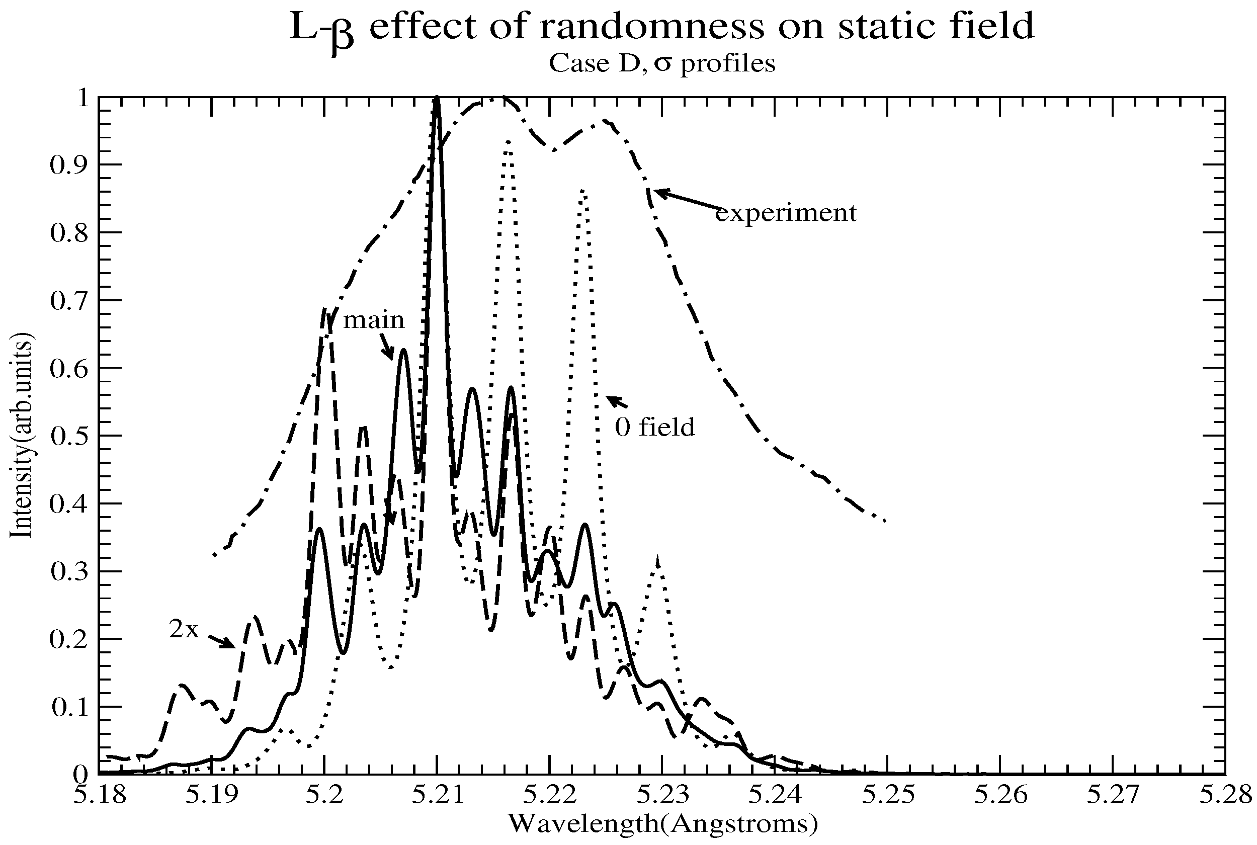
Figure 34.
Randomness of the static component perpendicular to the oscillatory field for , case D. Shown are profiles for the main calculation (solid line), the component perpendicular to oscillatory field 0 (0 field-dotted) and the component perpendicular to the oscillatory field but twice the size of that in the main calculation, i.e., 2 GV/cm (2x-dashed). The static component perpendicular to the oscillatory field is the same as in the main calculation, 1 GV/cm. Shown as well is the experimental profile (dashed–dotted line).
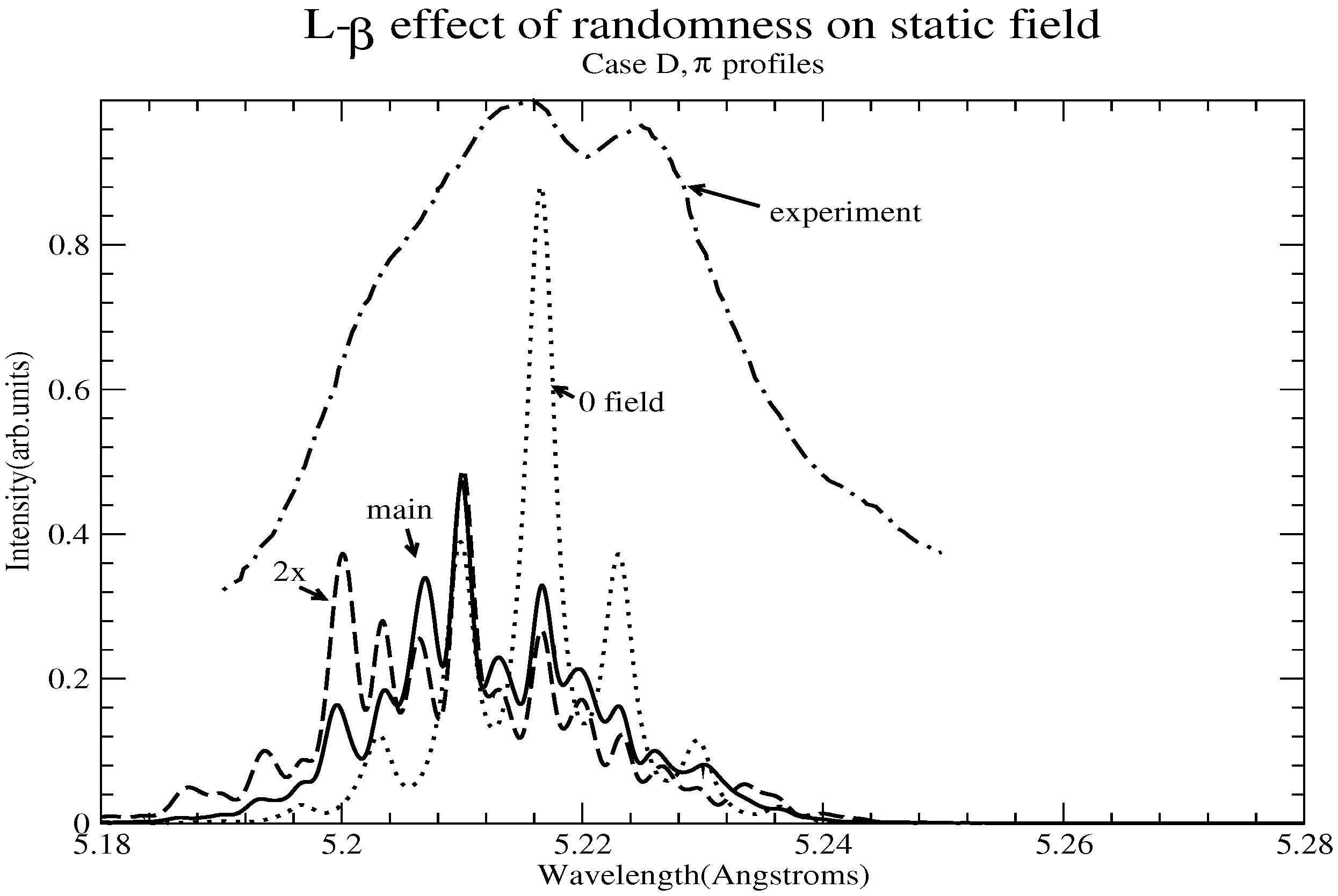
Figure 35.
Randomness of a static component perpendicular to the oscillatory field for , case D. Shown are profiles for the main calculation (solid line), the component perpendicular to oscillatory field 0 (0 field-dotted) and the component perpendicular to the oscillatory field but twice the size of that in the main calculation, i.e., 2 GV/cm (2x-dashed). The static component perpendicular to the oscillatory field is the same as in the main calculation, 1 GV/cm. Shown as well is the experimental profile (dashed–dotted line).
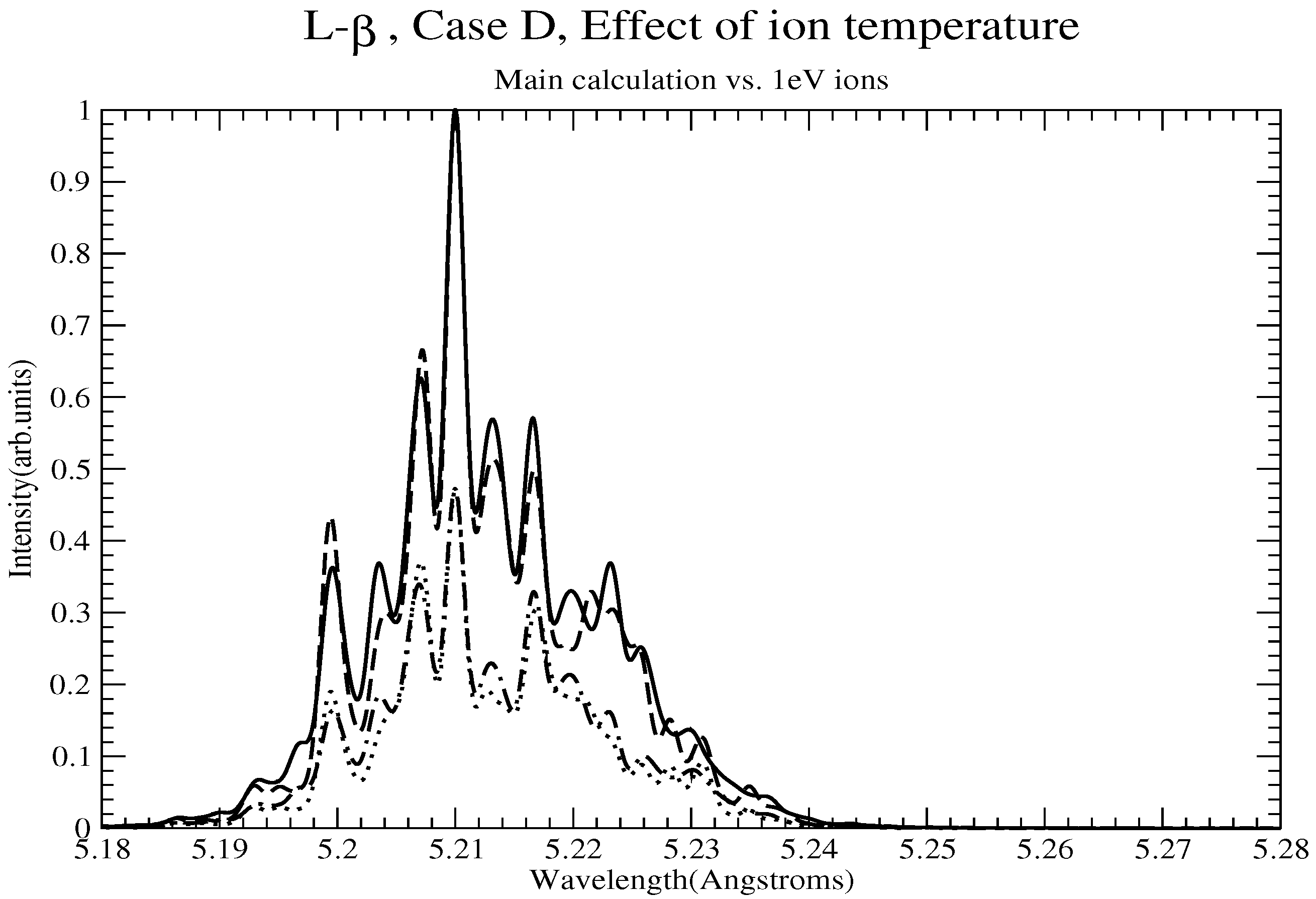
Figure 36.
(solid line) and (dashed–dotted line) main calculation profiles and the corresponding (dashed line) and (dotted line) profiles for an ion temperature of 1 eV.
Figure 36.
(solid line) and (dashed–dotted line) main calculation profiles and the corresponding (dashed line) and (dotted line) profiles for an ion temperature of 1 eV.
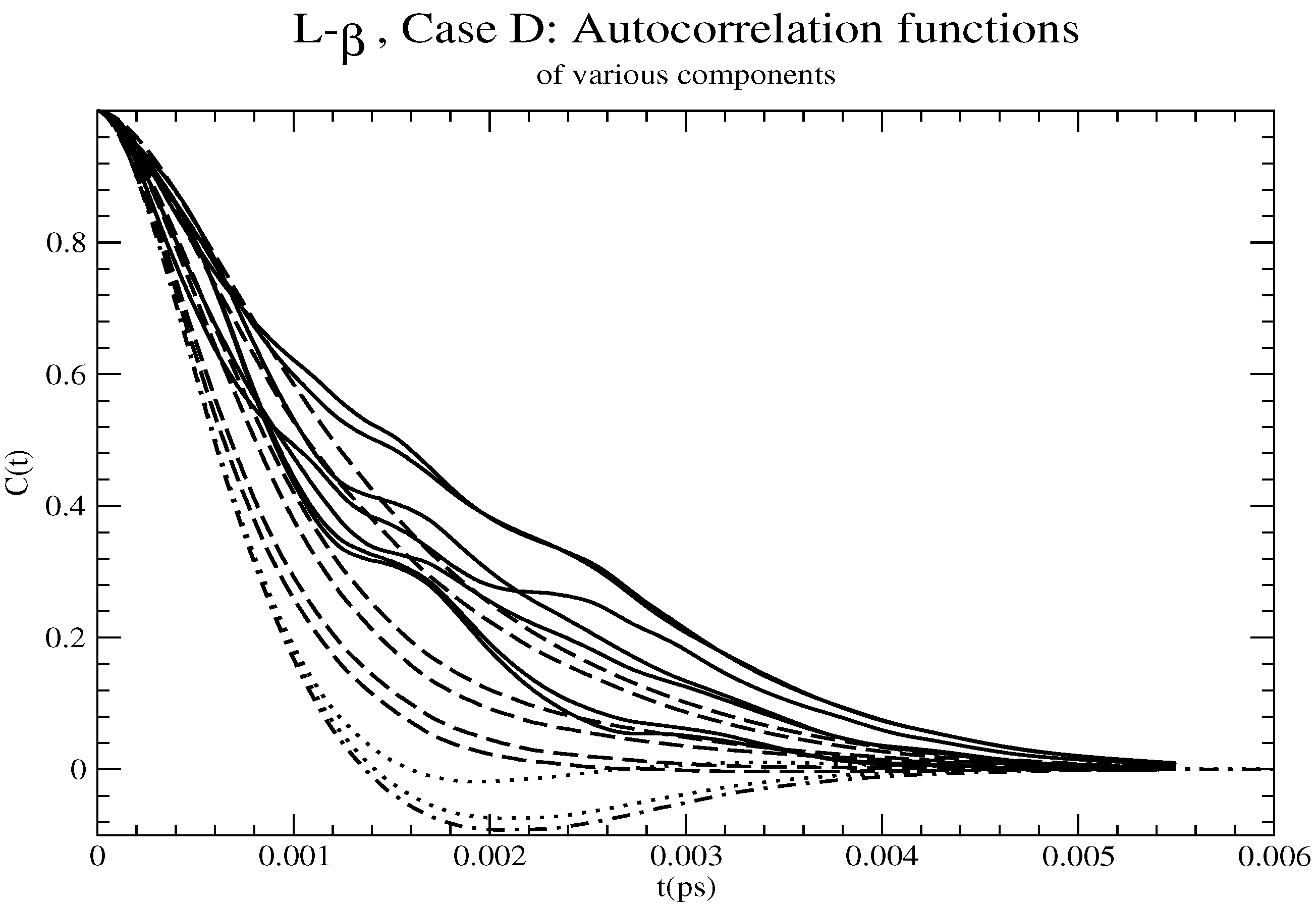
Figure 37.
Autocorrelation functions C(t) for the various components (corresponding to different Blokhintsev–Floquet peaks) of the , case D calculation. The solid lines correspond to the “main calculation” components, the dotted lines correspond to the two finely structured components in the absence of oscillatory and static fields. The dashed−dotted line corresponds to the calculation without fine structure and without oscillatory or static fields. The dashed lines are the components in the calculation where dressing was turned off.
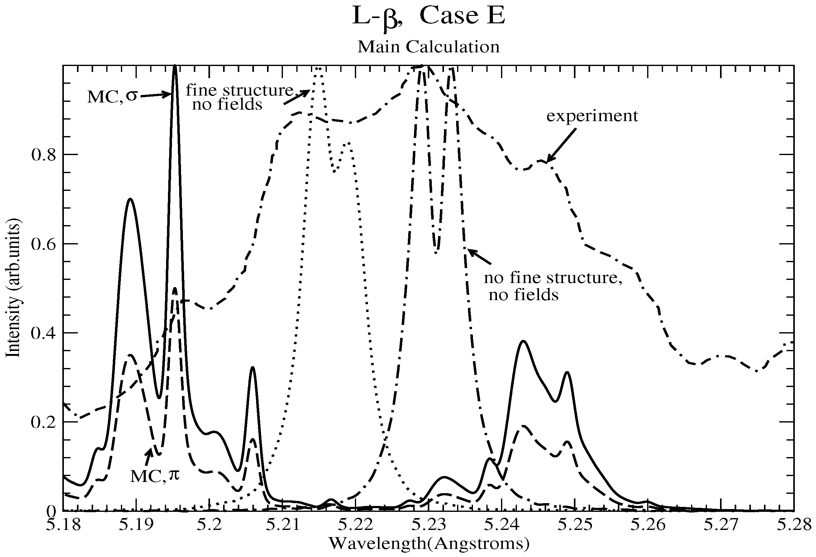
Figure 38.
Main calculation for
, case E. Shown are the
(solid line) and
(dashed line) profiles for the main calculation; profiles for the calculations without an oscillatory or static field, with (dotted line) or without (dashed–dotted line) fine structure; and the experimental profile (dot–double-dashed line) of Ref. [
10].
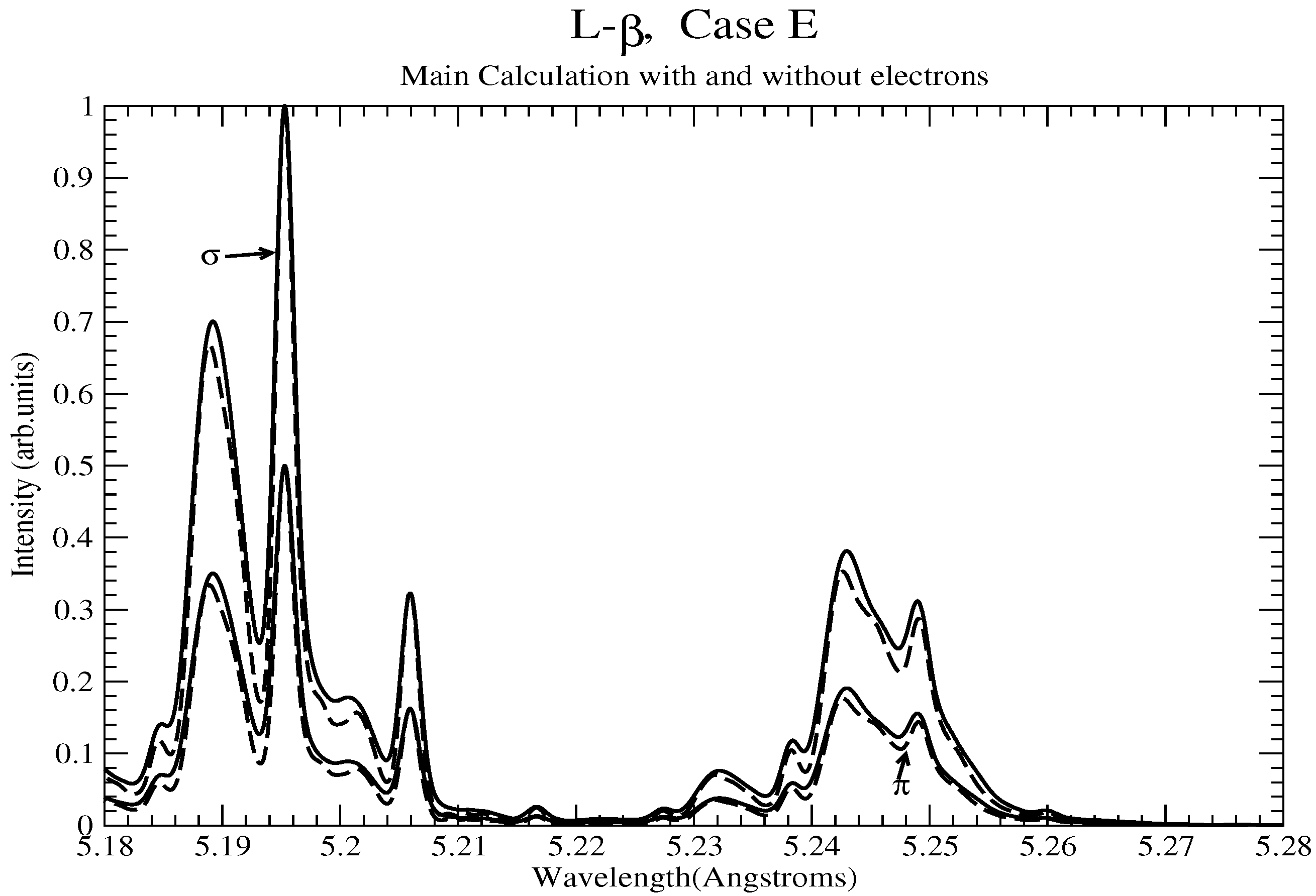
Figure 39.
Main calculation for , case E with only ion broadening accounted for (i.e., no electrons). Shown are the main calculation’s and profiles (solid line), together with the profiles for the calculations without electron broadening (dashed for the and dash–dot for the profile).
Figure 39.
Main calculation for , case E with only ion broadening accounted for (i.e., no electrons). Shown are the main calculation’s and profiles (solid line), together with the profiles for the calculations without electron broadening (dashed for the and dash–dot for the profile).
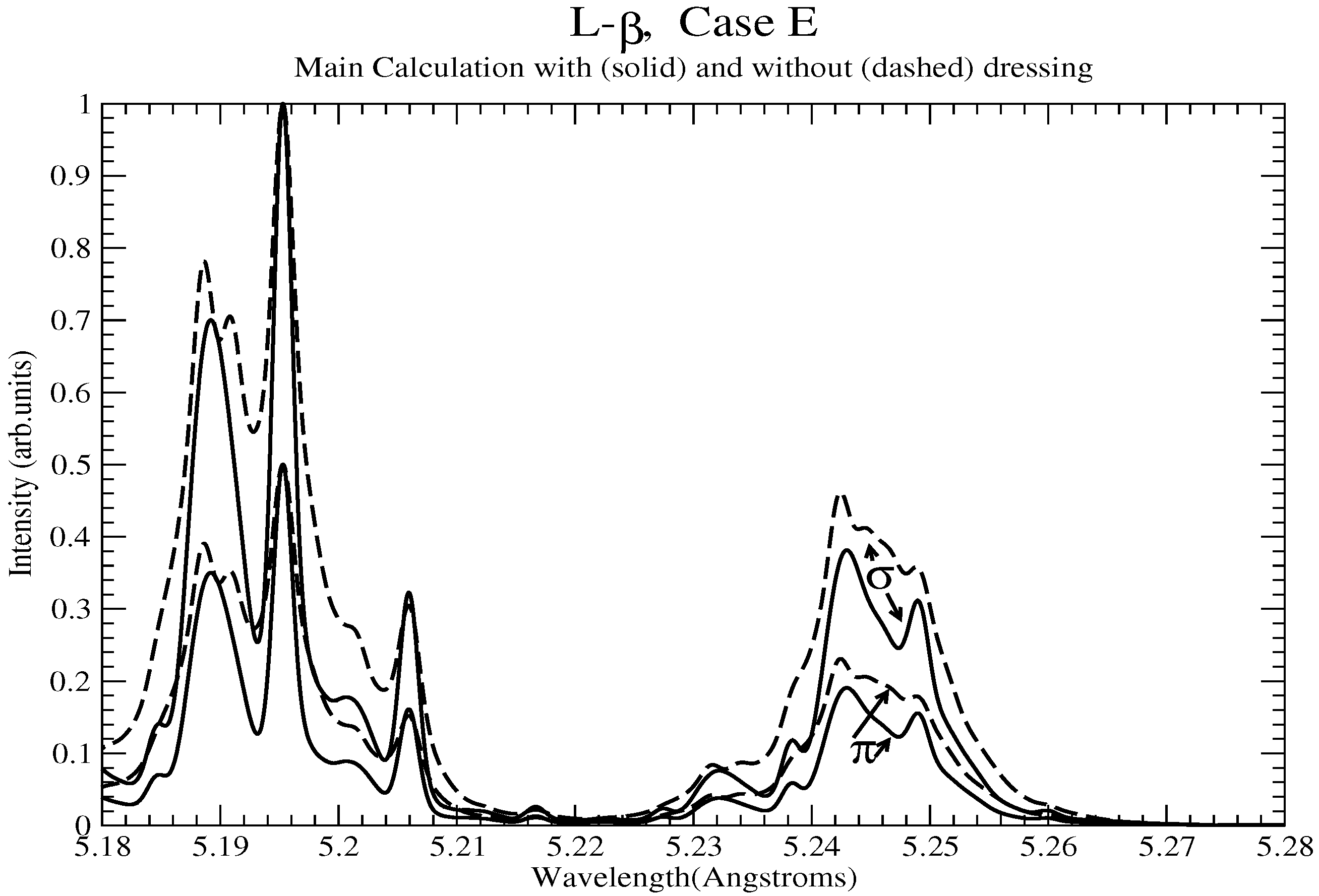
Figure 40.
Effect of dressing for , case E. Shown are and profiles for the main calculation (solid line) and the “no dressing” calculation (dashed line); i.e., the matrix S which describes the satellite positions and intensities is correctly computed, but the emitter–plasma interaction is (incorrectly) not dressed by the nonrandom static and oscillatory fields.
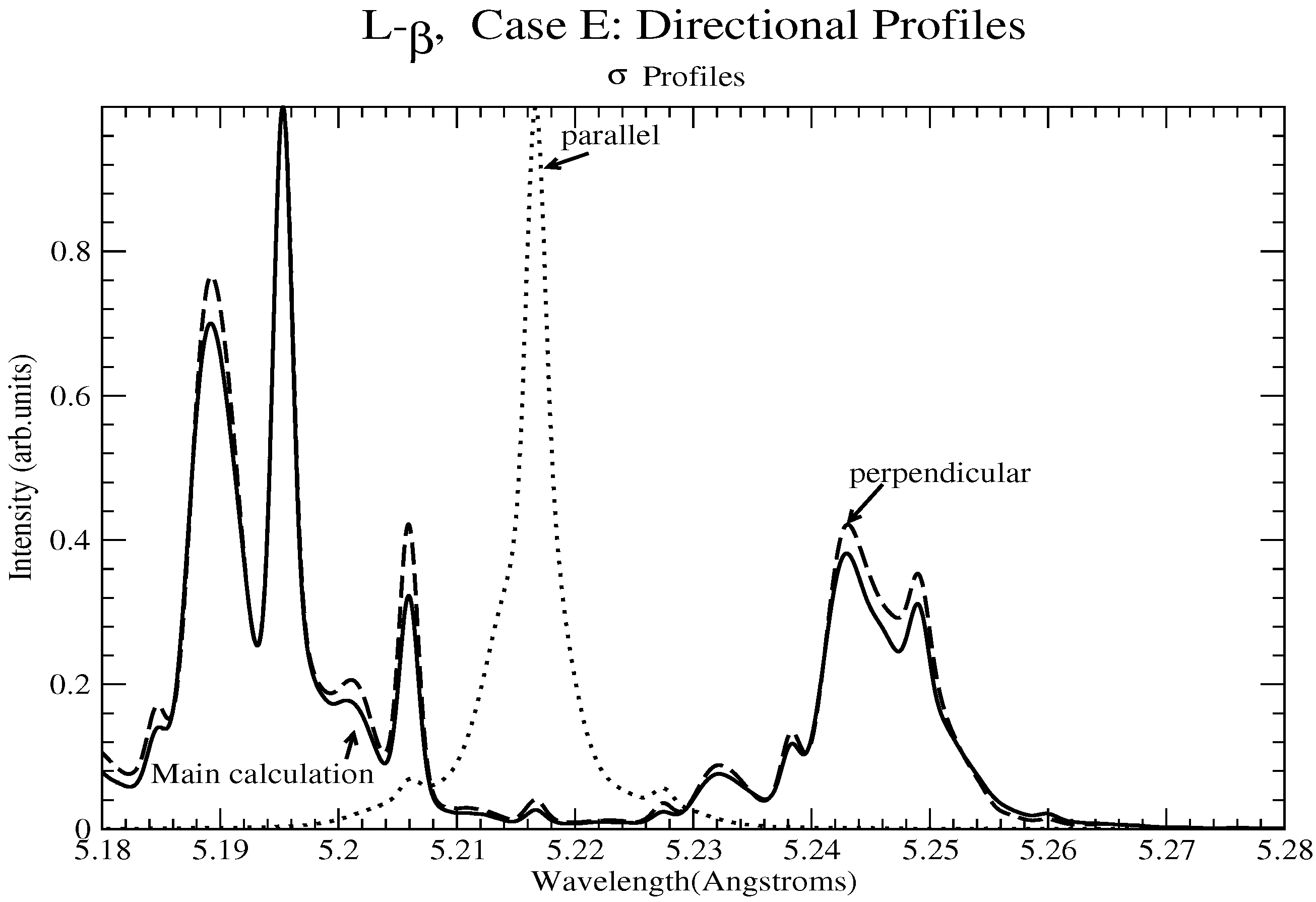
Figure 41.
Directional effects for , case E. Shown are profiles for the main calculation (solid line) and the entire static field (3.9 GV/cm) when parallel (dotted line) and perpendicular (dashed line) to the oscillatory field.
Figure 41.
Directional effects for , case E. Shown are profiles for the main calculation (solid line) and the entire static field (3.9 GV/cm) when parallel (dotted line) and perpendicular (dashed line) to the oscillatory field.
Figure 42.
Directional effects for , case E. Shown are profiles for the main calculation (solid line) and the entire static field (3.9 GV/cm) when parallel (dotted line) and perpendicular (dashed line) to the oscillatory field.
Figure 42.
Directional effects for , case E. Shown are profiles for the main calculation (solid line) and the entire static field (3.9 GV/cm) when parallel (dotted line) and perpendicular (dashed line) to the oscillatory field.
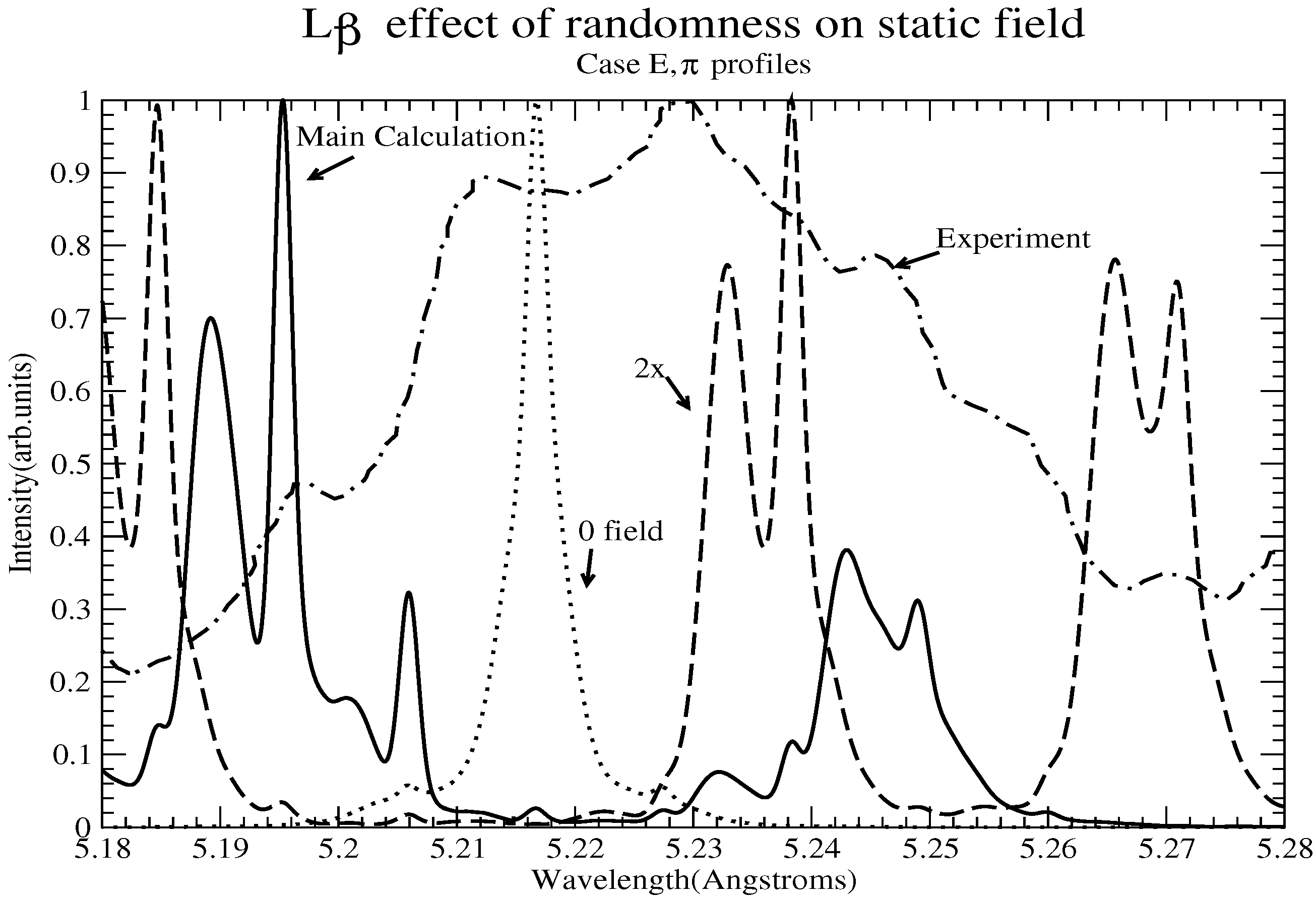
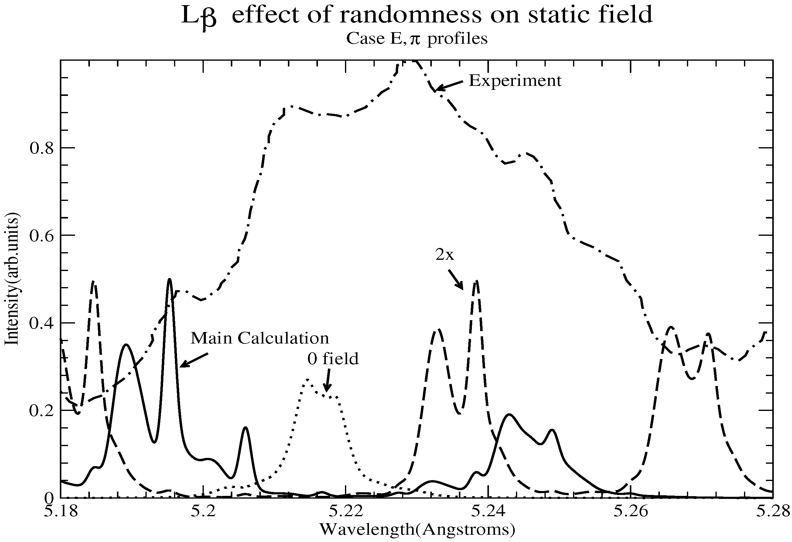
Figure 43.
Randomness of static component perpendicular to the oscillatory field for , case E. Shown are profiles for the main calculation (solid line), the component perpendicular to oscillatory field 0 (0 field-dotted) and the component perpendicular to the oscillatory field but twice the size of that in the main calculation, i.e., 6.696 GV/cm (2x-dashed). The static component perpendicular to the oscillatory field is the same as in the main calculation, 2 GV/cm. Shown as well is the experimental profile (dash−dotted line).
Figure 44.
Randomness of a static component perpendicular to the oscillatory field for , case E. Shown are profiles for the main calculation (solid line), the component perpendicular to oscillatory field 0 (0 field-dotted) and the component perpendicular to the oscillatory field but twice the size of that in the main calculation, i.e., 6.696 GV/cm (2x-dashed). The static component perpendicular to the oscillatory field was the same as in the main calculation, 2 GV/cm. Shown as well is the experimental profile (dash−dotted line).
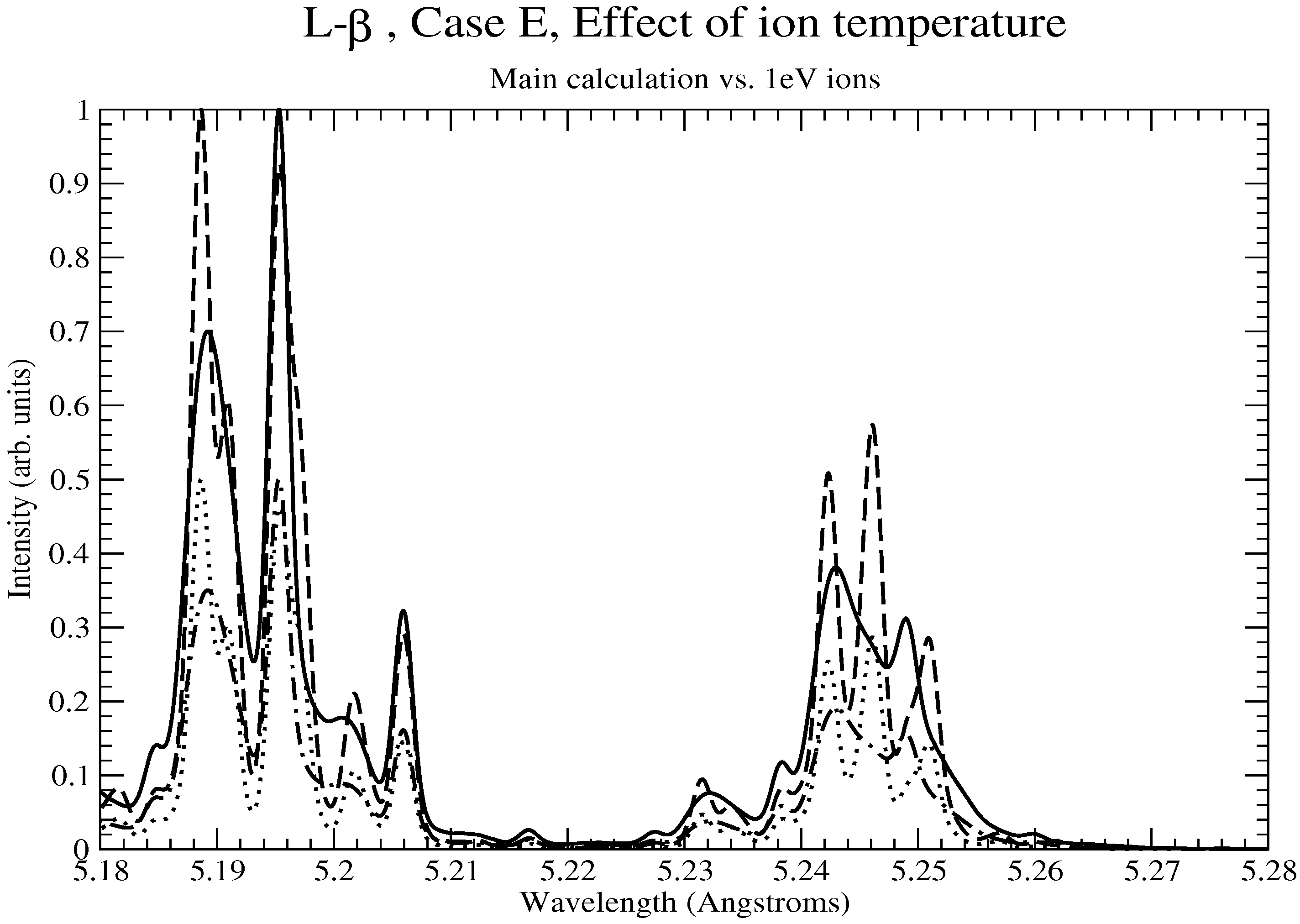
Figure 45.
(solid line) and (dashed–dotted line) main calculation profiles and the corresponding (dashed line) and (dotted line) profiles for an ion temperature of 1 eV.
Figure 45.
(solid line) and (dashed–dotted line) main calculation profiles and the corresponding (dashed line) and (dotted line) profiles for an ion temperature of 1 eV.
Figure 46.
Autocorrelation functions, C(t), for the various components (corresponding to different Blokhintsev−Floquet peaks) of the , case E calculation. Shown as well (dashed−dotted line) are the autocorrelation function for the calculation without static or oscillatory fields and with no fine structure, and the two components with fine structure but without any oscillatory or static fields (dotted line), i.e., normal calculations. The dashed lines display the corresponding autocorrelation functions without dressing.
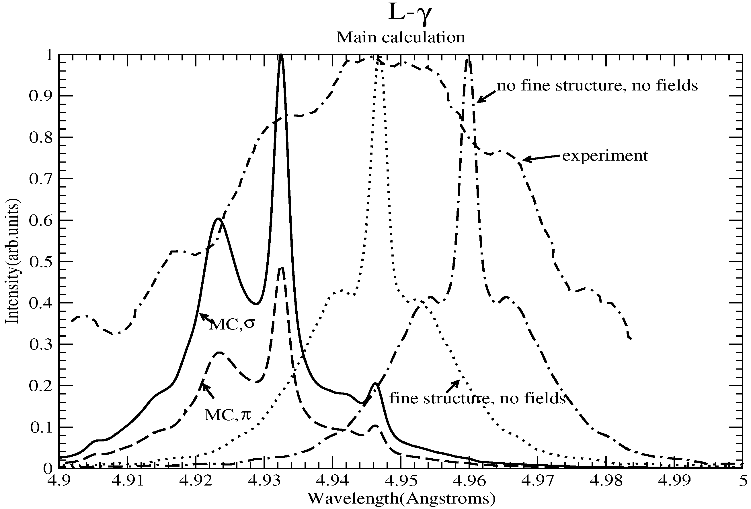
Figure 47.
Main calculation for
. Shown are the
(solid line) and
(dashed line) profiles for the main calculation, together with the profile without an oscillatory and static field with (dotted line) and without (dashed−dotted line) fine structure and the experimental profile (dot−double-dashed line) of Refs. [
9,
10].
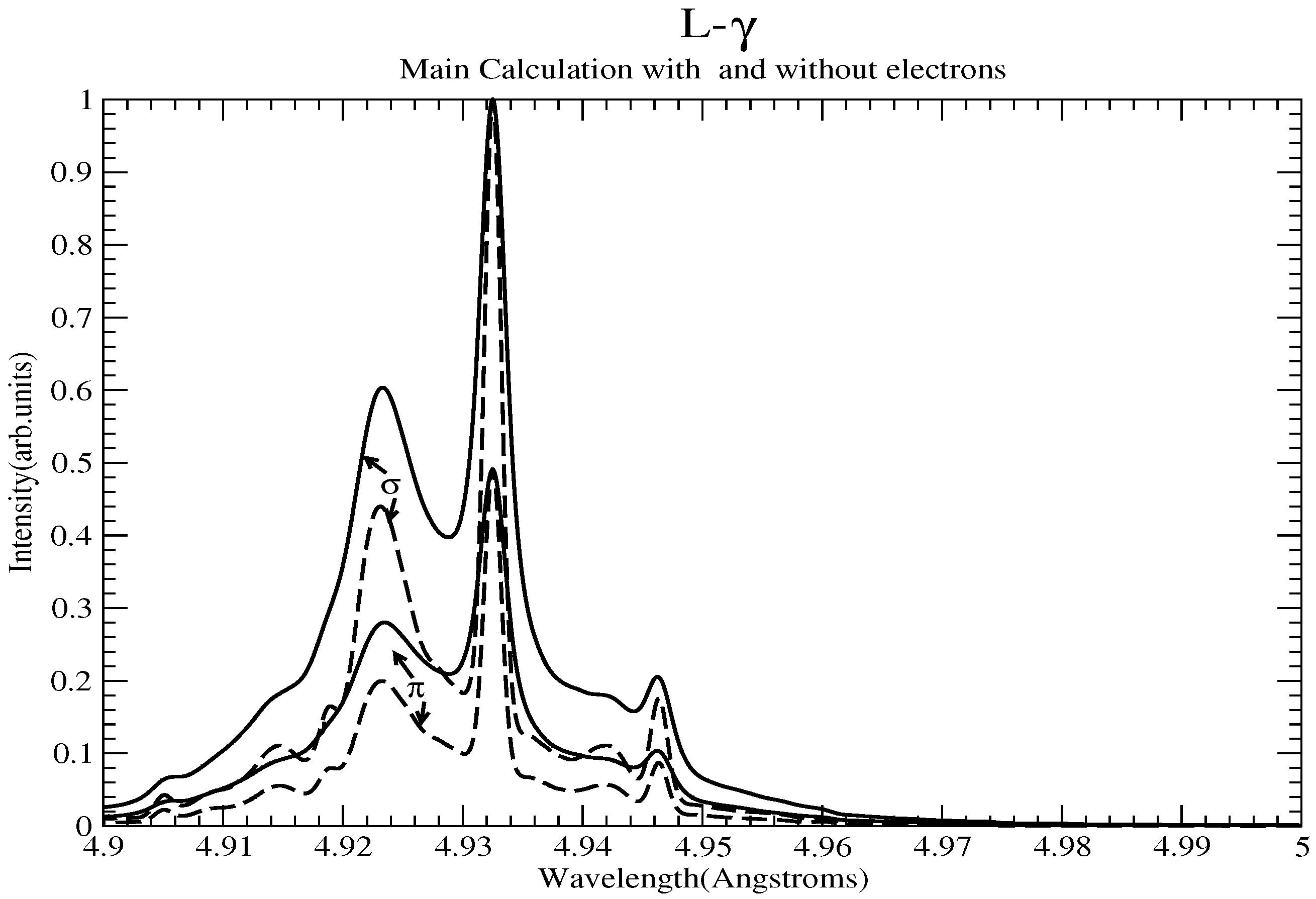
Figure 48.
Main calculation for with only ion broadening accounted for (i.e., no electrons). Shown are the main calculation and profiles (solid line), together with the profiles for the calculations without electron broadening (dashed).
Figure 48.
Main calculation for with only ion broadening accounted for (i.e., no electrons). Shown are the main calculation and profiles (solid line), together with the profiles for the calculations without electron broadening (dashed).
Figure 49.
Shown are and profiles for the main calculation (solid line) and the “no dressing” calculation (dashed line) for .
Figure 49.
Shown are and profiles for the main calculation (solid line) and the “no dressing” calculation (dashed line) for .
Figure 50.
Directional Effects for . Shown are profiles for the main calculation (solid line) and the entire static field (2.1 GV/cm) when parallel (dotted line) or perpendicular (dashed line) to the oscillatory field.
Figure 50.
Directional Effects for . Shown are profiles for the main calculation (solid line) and the entire static field (2.1 GV/cm) when parallel (dotted line) or perpendicular (dashed line) to the oscillatory field.
Figure 51.
Directional Effects for . Shown are profiles for the main calculation (solid line) and the entire static field (2.1 GV/cm) when parallel (dotted line) or perpendicular (dashed line) to the oscillatory field.
Figure 51.
Directional Effects for . Shown are profiles for the main calculation (solid line) and the entire static field (2.1 GV/cm) when parallel (dotted line) or perpendicular (dashed line) to the oscillatory field.
Figure 52.
Randomness of static component perpendicular to the oscillatory field for . Shown are profiles for the main calculation (solid line), the component perpendicular to oscillatory field 0 (0 field-dotted) and the component perpendicular to the oscillatory field but twice the size of that in the main calculation, i.e., 3.9 GV/cm (2x-dashed). The static component perpendicular to the oscillatory field is the same as in the main calculation, 1 GV/cm. Shown as well is the experimental profile (dashed–dotted line).
Figure 53.
Randomness of the static component perpendicular to the oscillatory field for . Shown are profiles for the main calculation (solid line), for the component perpendicular to oscillatory field 0 (0 field-dotted) and for the component perpendicular to the oscillatory field but twice the size of that in the main calculation, i.e., 3.9V/cm (2x-dashed). The static component perpendicular to the oscillatory field is the same as in the main calculation: 1 GV/cm. Shown as well is the experimental profile (dashed–dotted line).
Figure 54.
(solid line) and (dashed–dotted line) main calculation profiles and the corresponding (dashed line) and (dotted line) profiles for an ion temperature of 1 eV.
Figure 54.
(solid line) and (dashed–dotted line) main calculation profiles and the corresponding (dashed line) and (dotted line) profiles for an ion temperature of 1 eV.
Figure 55.
C(t) for the strongest components (i.e., combinations of Floquet and Blokhintsev positions).
Figure 55.
C(t) for the strongest components (i.e., combinations of Floquet and Blokhintsev positions).
Table 1.
Ly- calculation parameters.
Table 1.
Ly- calculation parameters.
| Calculation | El.Density () | T (eV) | F (GV/cm) | (GV/cm) | Ref. |
|---|
| A | 22 | 600 | 4.8 | 0.7 | Figure 5a in [10] |
| B | 22 | 550 | 4.4 | 0.5 | Figure 5b in [10] |
| C | 22 | 600 | 4.9 | 0.6 | Figure 5c in [10] |
| D | 6.6 | 550 | 1.41 | 2 | Figure 5d in [10] |
| E | 17.4 | 500 | 3.9 | 1 | Figure 3b in [10] |
Table 2.
Ly- calculation parameters.
Table 2.
Ly- calculation parameters.
| El.Density () | T (eV) | F (GV/cm) | (GV/cm) | Ref. |
|---|
| 36 | 500 | 2.1 | 0.6 | Figure 3A in [10] |


