Abstract
An extension of the variational approach for the study of atomic properties of ions and atoms containing up to 10 electrons is presented. The study includes exact analytical calculations of all the interaction terms, including direct Coulomb interactions and exchange interactions. Two alternative formulations are considered, with one and with two variational parameters. The exact and numerical values of these parameters are obtained and tabulated. The results of this study are compared with Hartree–Fock calculations. Sample applications to electron-atom scattering and energy losses of ions in Tokamak plasmas are presented.
1. Introduction
Throughout the years, great advances in the knowledge of the atomic structure and atomic processes involving ionized matter have been made. Today, the question of atomic modeling is a well-developed area where a large number of relevant works has been published. Detailed accounts of early and more recent advances may be found in [1,2,3,4,5,6,7]. Current theories include statistical descriptions, numerical studies based on Hartree–Fock theory, and density-functional methods. On one side, the structure of one- and two-electron atoms has been studied in great depth [8]. On the other, statistical theories have been able to describe the general properties of many-electron atoms [9]. In particular, the Thomas–Fermi and related statistical models provide useful approaches to describe extreme cases, ranging from atomic systems [10] to astrophysical environments [11]. Between these extremes, the case of few-electron atoms remains a more elusive area, where no simple analytical solutions are readily available, and most studies refer to numerical methods such as Hartree–Fock calculations [4,12].
In this context, there is a need for analytical methods that could provide more straightforward access to problems related to few-electron atoms or ions in matter. This includes, in particular, the areas of ions in plasmas. A large number of atomic processes in dense and dilute plasmas bear great interest for nuclear fusion studies, such as those related to Tokamak or ICF-type plasmas [13,14,15,16,17,18,19,20,21], ion acceleration in plasmas by ultra-short laser pulses [22], astrophysical media such as stellar interiors [23], where highly ionized matter is created [24,25], as well as in space science [26]. Other areas of great relevance are those of radiation therapy and other applications using energetic ion beams [27,28,29,30].
As mentioned before, there is always the Hartree–Fock (HF) method, but HF calculations are expensive in terms of computer time. Therefore, if alternative methods that could provide fast and reliable results were available, they would become useful tools in quite different areas of knowledge.
One well-known and simple approach is the variational method of Ritz [5,31], but applications to atomic systems have been, so far, mostly limited to the normal or the excited states of He and to hydrogen-like atoms. A more recent and interesting development was made by Kaneko [32], who extended the variational calculation to atoms of Li and Be.
The purpose of this work is to make a further advance in the line of variational calculations, extending the study to ions and atoms containing up to 10 electrons. The aim is not to compete with the more elaborate and precise computer calculations but to develop a simplified analytical approach that could allow straightforward applications to many problems of atomic interactions in matter.
This includes, for instance, problems of electron scattering by ions or neutral atoms, X-ray scattering in matter, the penetration of ions in solids, and some relevant problems of ions in fusion plasmas such as those already mentioned, the behavior of impurity ions in the laboratory or astrophysical plasmas, or the use of ion beams for medical or technological applications.
This work is organized as follows: in the next section, a brief summary of the variational method is made. The following sections describe the extension of the method to include , , and electrons, obtaining exact analytical expressions for all the electron-interaction energies, including direct and exchange terms. Using the exact expressions for the energy terms, the variational parameters are determined, and their values are tabulated, covering a total number of 45 cases of ions and atoms. The results of this approach will be compared with those obtained from the HF theory, considering the calculations of total energies, densities, and form factors and ending with two sample applications: elastic scattering of electrons by atoms and stopping of ions in Tokamak-like plasmas.
Two appendices condense further information: Appendix A describes the method used for the analytical calculation of electron interaction integrals, and Appendix B contains all the values of interaction-energy terms obtained from the exact analytical integrations.
2. Variational Method
The energy of an atom or ion of atomic number Z with an N-bound electron may be represented in the form
where H is the Hamiltonian and is a determinantal wave function.
The Hamiltonian consists of one- and two-electron operators, and respectively, of the form [5]:
being in this case:
An important property to be used here is that the expectation value of the whole Hamiltonian with the determinantal wave function may be decomposed in a sum of simple one-orbital and two-orbital elements as
where denotes the individual wave functions of electrons. The first term in represents the usual Coulomb interaction between electrons, while the second term corresponds to the exchange interactions between electrons with equal spin projections.
Using the properties of one- and two-electron operators, the energy may be separated in the following way
where is the kinetic energy of all electrons, is the sum of the electron–nucleus interactions, and and represent the direct and exchange electron interactions, = and .
In order to apply the variational method, the electron wave functions must contain one or more parameters whose values are determined by minimizing the energy. Moreover, to obtain the expressions for the variational energy, according to Equation (1), the expectation values were calculated by applying Hund’s rules and considering the Slater determinant with maximum and compatible with those rules, as described in Section 4.
2.1. Wave Functions and Densities
The wave functions used in this formulation are parameterized hydrogenic wave functions of the form
with the corresponding densities
where
I have assumed here two variational parameters (for 1s and 2s wave functions) and (for 2p wave functions), using for simplicity related parameters , .
It should be noted that in order to obtain meaningful results from the variational method, the trial wave functions must be orthogonal. For this reason, the and orbitals must have the same variational parameter. However, this restriction does not apply to the orbitals since the orthogonality with s states is guaranteed by the corresponding angular integrals. This degree of freedom is quite useful for obtaining a better variational solution, as will be shown here.
3. Calculation of Energy Terms
The first question that we face here is the calculation of kinetic and interaction-energy terms in Equation (8). The first two terms (T and ) are straightforward; the problem lies in the other two terms ( and ) corresponding to electron–electron interactions. These are the nontrivial terms to be calculated in this work.
I will write down now the values of the first two terms (T and ). The calculation of the electron–electron interaction terms will be described in Appendix A.
3.1. Kinetic Energy Terms
The kinetic energy terms are those already known for hydrogenic wave functions, namely (energy values here are expressed in atomic units)
The latter expression for corresponds to the formulation in terms of two parameters, and ; in the case of restricting the formulation to only one parameter , the values of and are equal: .
3.2. Electron–Nucleus Interaction
The calculation of these terms is also straightforward, with the results
Here, for easier identification of the various energy terms, I have introduced the letter U to represent the electron–nucleus interactions (with positive values); the upper-script will no longer be necessary. Therefore, in the following, the letters U, V and W will identify the energy terms corresponding to electron–nucleus, electron–electron (direct terms) and electron–electron (exchange terms), respectively.
Again, in the case of using only one parameter (), the expression for coincides with , i.e.,
3.3. Electron–Electron Interactions
Due to the identity of electrons, we have to consider two types of interaction terms. On the one side, we have direct Coulomb interactions; the calculation of these terms is made using the expression
On the other hand, the exchange interaction between orbitals i and j is calculated as
To evaluate these integrals, I will use the representation of in terms of spherical harmonics , namely [33],
and using the property (with :
Considering all the possible occupied orbitals involved in this study, a number of different integrals related to electron interactions must be calculated. The analysis becomes, in practice, complicated by the growing number of interactions that appear when the number of electrons increases. The handling of the corresponding integrals becomes rather cumbersome; however, an important aspect of the variational method using hydrogenic wave functions is that all those integrals can be calculated analytically and yield exact algebraic values. The details of these calculations are described in Appendix A, and the complete set of results is given in Appendix B.
4. Expressions for the Energies
The energy of an atomic system is formally given by Equation (8), but the number of terms that must be included depends strongly on the number of electrons attached to the atom or ion. The results for all the individual energy terms are given in Appendix B. These results must be combined in a way that depends on the distribution of electrons to obtain appropriate expressions for the variational energy of each atom or ion.
To start with a simple case, I will first consider the Be atom. The electronic structure of the neutral atom is of form Hence, in this case, one must take into account all the electron–electron interactions that take place between the and orbitals. This yields the expression for the total energy of this atom:
which contains a total of 16 terms. Here, I introduce the notation to indicate the electronic structure of the atom.
Similarly, I will use the compact notation to denote the electronic structure of the various Be ions (notice that stands simply for a point nuclear charge ). This notation will extend to all the ions covered by this study.
It may be noticed that insofar as the electronic structure is concerned, all ions belonging to the same isoelectronic series contain the same terms in the expression for the corresponding energies. We may state this property by writing relations such as and so on with other isoelectronic series.
For heavier elements, where the orbitals are progressively occupied, the number of terms in the expression for the total energy increases steeply. The energy of these heavier ions may be expressed in compact form using the configuration as a basis, namely
where contains all the energy terms associated with occupied orbitals, including the interactions of states with and . The occupation of these orbitals is made according to Hund’s rule. In addition to maximum S and maximum L (compatible with the first rule), the occupation of the orbitals is considered here with the additional criterion of maximum and maximum . This guarantees that one can work with only one Slater determinant [4,5], which eases very much the calculations. In all cases, the calculations apply to the ground state.
To illustrate this point, in Table 1, I collate several examples. The numbers in the columns indicate the number of terms of each type that should be added to the sum to obtain the total energy of particular atoms or ions. Thus, in the case of Ne, taking the structure of (Equation (28)) as a starting reference, the total energy becomes:
which contains a total of 85 terms (including the 16 terms of ). It may be shown, however, that only 19 of these terms are different.

Table 1.
Number of Energy Terms for various sample cases.
One may also notice in this table that the are no terms of type because of the Pauli principle. Therefore, the corresponding places in the Table are void (this term is included only to maintain the ordering and symmetry of the table).
Some particular cases in this table that illustrate the isoelectronic equivalence are those of with with and with , where the sequence of numbers for each of these pairs of elements are the same. Interestingly, the difference in the energies of cases within the same isoelectronic series is produced only by the electron–nucleus interaction, which depends on the atomic number
For further and more detailed analysis I give in Appendix B the complete expressions of the variational energy for all the possible charge states of , which also yields the expressions for all the other elements with when the properties of isoelectronic series are applied.
5. Determination of the Variational Parameters
5.1. One Variational Parameter (V1 Formulation)
I will first consider the simplest formulation in terms of one variational parameter , so that, in this case, . This will be referred to as the “V1 formulation”.
Once the set of terms that contribute to the energy of each ion and atom are determined, and having also determined the exact algebraic values of each term as a function of parameter (by Equations (18)–(23) and the equations in Appendix B), it is possible to determine the value of by minimizing the variational energy in each case. This can be made in a straightforward way by noticing that the kinetic energy is a quadratic function of , while all the other terms have a linear dependence on this parameter. Hence, the expression for the total energy is in all cases of the form
where , and are the appropriate coefficients corresponding to the total kinetic energy (), electron–nucleus interaction energy (), and direct and exchange electron–electron interaction energies (), and where the dependencies on the parameter and nuclear charge Z have been explicitly factorized.
This expression makes it obvious that the value of that minimizes the energy is
Let us consider, for example, the case of carbon atoms, In this case, according to Equations (18)–(23) and those of Appendix B, and the numbers in Table 1,
Substituting this into Equation (32) and arranging terms, we get a long but exact expression for the value of
with in this case.
Finally, after some algebraic work and the cancellation of common factors, one gets
A similar treatment can be made for all the possible ions and atoms in the range , obtaining, in all cases, exact algebraic values for the corresponding parameter The complete set of numerical values is collated in Table 2. The table contains all the cases of possible charge states n, from to ; the latter case corresponds to ions carrying only one electron so the value of is just Z (hydrogen-like ions). The total number of cases described is 55 (or 45 if the obvious cases with are excluded), which covers all the possible atoms and ions in the prescribed range of Z values.
Table 2.
Variational parameter (in atomic units).
By observing the results in this table, one finds some interesting regularities: the values in the diagonals, when reading them from left to right, increase from one place to the next by exactly 1. It can be seen that this is a property of the electronic structure of ions belonging to the same isoelectronic series. For these cases, the sequence of occupation numbers for the whole series is the same; therefore, the values of may be expressed in a way similar to Equation (37), which starts with the value of Z (with the rest of numbers being the same for the whole isoelectronic series).
As a consequence of this property, one realizes that it would be enough to determine the values of for all the charge states of Ne (with n from 0 to 9) to obtain the values of for the rest of the cases in the table.
Unfortunately, this regularity applies only in the one-parameter formulation. Instead, in the following description, in terms of two parameters, each ion or atom must be solved as a particular case.
5.2. Two Variational Parameters (V2 Formulation)
I consider now an extension of the variational calculation using two parameters. This approach will be referred to as the V2 formulation. As noticed before, an important condition of the variational method is to assure the orthogonality of the trial wave functions. In the present study, I take advantage of the automatic orthogonality between the s and p orbitals that arises from the angular dependencies. In addition, the three p-type orbitals must be mutually orthogonal. To assure these conditions, I use a set of hydrogenic p orbitals containing a common variational parameter
Therefore, I will keep the parameter for the and orbitals, according to Equations (9) and (10), and introduce parameter for the wave functions, according to Equations (11) and (12), and the related densities given by Equations (15) and (16) (and with auxiliary parameters , ).
The calculation of the direct and exchange interaction terms is now much more cumbersome. Some details of these calculations are given in Appendix A and the resulting values in Appendix B.
With this new scheme, the expression for the variational energy depends now on both and : . The values of and were then determined by minimizing ) with respect to both parameters. To find the optimum values of these parameters, a detailed study of the function ) in the – plane must be made. This was performed in a numerical way, and the results are given in Table 3. The void places in this table correspond to electronic configurations that involve only and orbitals (so in these cases, ).
Table 3.
Variational parameters .
Figure 1 shows an example of the case of with charges varying from 0 to 9. The black dots are the results of the one-parameter formulation (V1 case), and the blue dots are those of the two-parameter formulation (V2 case). For charges larger than five, the three curves collapse into a single one; the reason for this is that for these higher charge values all the -shell electrons are removed, and so the calculation restricts to the one-parameter case.
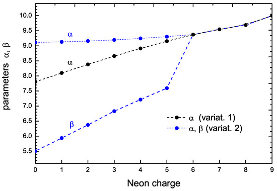
Figure 1.
Parameters and for with charges varying from 0 to 9. The black dots are the results of the one-parameter formulation (V1 case), and the blue dots are those of the two-parameter formulation (V2 case).
The figure also illustrates an interesting feature: when the possibility of two parameters occurs (i.e., from charge 0 to 5), the values of increase (with respect to the one-parameter formulation) and the new parameter appears with a much lower value. This corresponds to the physical feature that the and orbitals move inward (approaching the nucleus) while the orbitals move outward (with respect to the one-parameter description). The result of this is that the interaction energy between these electrons decreases, as well as the total energy. (There are other terms, such as the kinetic energy of s orbitals, whose value increases, but it may be shown that the main difference is the reduction in the electrostatic interaction between s and p orbitals due to the largest spatial separation.) Thus, the additional degree of freedom arising from the availability of the two parameters gives the possibility of lowering the total energy.
Figure 2 illustrates how this readjustment of parameters takes place, and the ensuing shift in the value of . The dotted curve in this figure shows the values of the energy corresponding to the V1 scheme. The optimum value of , in this case, is 7.807, and the corresponding variational energy is −121.9 a.u. On the other hand, the solid line shows the values of the two-parameter energy , for a fixed value of , as a function of . In this figure, the value of was fixed at the optimum value, 5.508, obtained by a numerical iterations procedure. This curve indicates an increase in the optimum value resulting in 9.113, leading to a lower energy, a.u., which is closer to the Hartree–Fock energy, a.u., here represented by the lower red dashed line. The difference between these two values is 1.6 %.
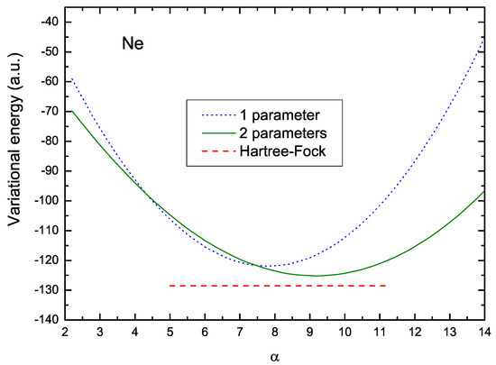
Figure 2.
Variational energy as a function of parameter for the V1 and V2 formulations. The dotted curve in this figure shows the values of the energy corresponding to the V1 case; the solid line shows the values of the energy for the V2 case and for a fixed value of . The red dashed line represents the HF value.
Therefore, it is expected that the two-parameter variational formulation will yield a better description of the electronic structure of the atoms and ions. In the following, we will test the degree of improvement by comparing it with precise atomic structure calculations.
6. Variational Results, Comparisons and Applications
The results of the variational minimization of the energy expressions for each of the atoms and ions included in this study are condensed in Table 2 (one-parameter cases) and Table 3 (two-parameter cases). The changes in the parameter values have been analyzed, and the next question is to compare them with the precise results obtained from the numerical solutions of the Hartree–Fock equations. For this purpose, I will use here the set of results tabulated by Clementi and Roetti [12].
6.1. Total Energies
The first critical test of the variational calculations is to compare the values of the total energy with those obtained from the solutions of the Hartree–Fock (HF) equations.
Figure 3 shows the values of the variational energy obtained with the one-parameter (V1) and two-parameter formulations (black and blue lines, respectively) for Be, C, O, and Ne with various charge states. The red dots in this figure are the HF values obtained from Ref. [12]. As may be observed, the variational results agree very closely with the HF values. The maximum deviation from the HF values occurs for , with differences of for the V1 case, and for the V2 case (this case corresponds to the one illustrated in Figure 2). As shown in the figures, the results of the V2 formulation are in excellent agreement in all cases.

Figure 3.
Comparison between energy values resulting from variational calculations using 1 and 2 parameters and those from the Hartree–Fock calculation for neutral atoms (Q = 0) and for ions with charge Q = 2 and Q = 4.
6.2. Densities and Form Factors
Before entering into this analysis, it is appropriate to introduce the formulas for the form factors corresponding to the present formulation.
As is known, the form factors are defined by the Fourier transform of the electron density, in the form
Considering the densities of the , , and orbitals of interest in this work, the following expressions for the corresponding form factors are obtained:
To obtain the expression for the function , I have taken the angular average of the corresponding density; in this way, the average form factors for the and become equal.
The form factor for the whole atom or ion is then defined by
where , and are the occupation numbers of each orbital.
Figure 4 shows the form factors corresponding to the , , and orbitals of Oxygen, obtained with the one- and two-parameter formulations. The features illustrated in this figure are a consequence of the previously described readjustment of atomic orbitals when switching from the one-parameter (dotted lines) to the two-parameter (solid lines) approach. The and curves shift to larger values of q (corresponding to the orbitals that move radially inward in space), while the curve shows the opposite behavior. The largest effect is found in the form factor due to the much lower value of the parameter with respect to shown in Figure 1. The final result of these readjustments is a total form factor that compares very well with the HF form factor (open circles in this figure).
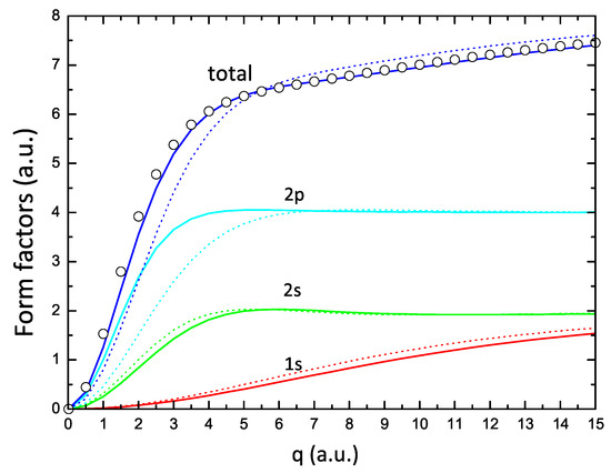
Figure 4.
Form factors corresponding to , , and electrons obtained from the one-parameter (dotted lines) and two-parameter (solid lines) formulations, and the corresponding total form factors for Oxygen; the circles are the values of the form factor obtained from the HF calculations of Ref. [12].
A different model to calculate the form factors for atoms and ions, frequently used in the area of ion–solid interactions, is the Brandt–Kitagawa model (BK) [34,35]. This model is based on the statistical properties of high-Z atoms [9]. For this reason, it may not be expected to yield accurate results for relatively low-Z elements (as is the present case), where the shell structure is a notorious feature.
In the BK approach, the form factor is given by.
where N is the number of electrons and is a screening parameter given by
Figure 5 compares the values of the radial densities, defined as (upper two panels) and form factors (lower two panels) for and . The curves in panels (a) and (b) show significant differences in the electron densities with respect to the HF results (with some mild improvement in the V2 curves). However, the corresponding form factors shown in panels (c) and (d) provide a distinct view. The form factor obtained from the V1 formulation compares fairly well (considering the simplicity of the approach) with the HF form factor, while the V2 curve shows an almost excellent comparison with the HF curve.
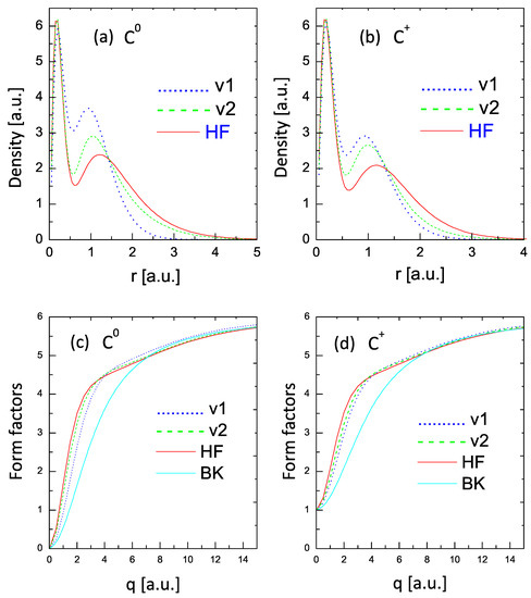
Figure 5.
Radial densities (upper panels) and form factors (lower panels) for and . Dotted lines: one variational parameter; dashed lines: two variational parameters; solid red lines: HF values. The lower (BK) lines in panels (c,d) are the form factors calculated with the statistical model of Ref. [34].
This tendency of a much better comparison of the form factors than of the densities with the HF results was obtained in all the cases covered by this study.
The two additional curves depicted in the figures denoted as BK are the form factors obtained from the Brandt–Kitagawa model [34]. These results confirm the expectation that the statistical models may fail for low-Z elements [9].
Further examples and comparisons of form-factor behavior are shown in Figure 6, which depicts the cases of , , , and . For , the one-parameter V1 curve deviates significantly from the HF one but shows an improvement for higher charge states. The two-parameter V2 curves show an excellent agreement with the HF values in all cases. On the other hand, the BK curves show deviations from the more correct values.
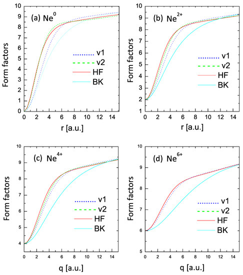
Figure 6.
Form factors for , , , and . Dotted lines (v1): one-parameter case; dashed lines (v2): two-parameter case; solid lines: HF results; BK lines: statistical model of Ref. [34].
7. Sample Applications
7.1. Electron Scattering
The amplitude of elastic scattering of electrons by a spherical-averaged potential is given by [36]
where is the Fourier transform of the scattering potential, q is the momentum-angle variable: with , and v is the electron speed.
Using the relation between and the form factor , the expression for the differential cross-section becomes:
or introducing the scattering intensity (in atomic units):
Pioneering calculations of electron scattering by atoms based on HF form factors have been reported by Mott and Massey [36].
In Figure 7, I show the values of the scattering intensity for atoms of Be, C, O, and Ne. The curves are the results of the present variational model (according to the V2 formulation), while the dots are the HF values tabulated in Ref. [36], rescaled to the present format. An excellent agreement between these fully independent calculations is found over a wide range of values.
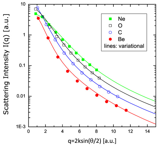
Figure 7.
Scattering intensity of electrons in Be, C, O, and Ne, according to Equation (48). The symbols are the calculations reported in Ref. [36]; the lines are the results of the variational calculations with two parameters.
Finally, the variational results are presented in Figure 8 in the form of , showing the asymptotic convergence to the Rutherford limit .
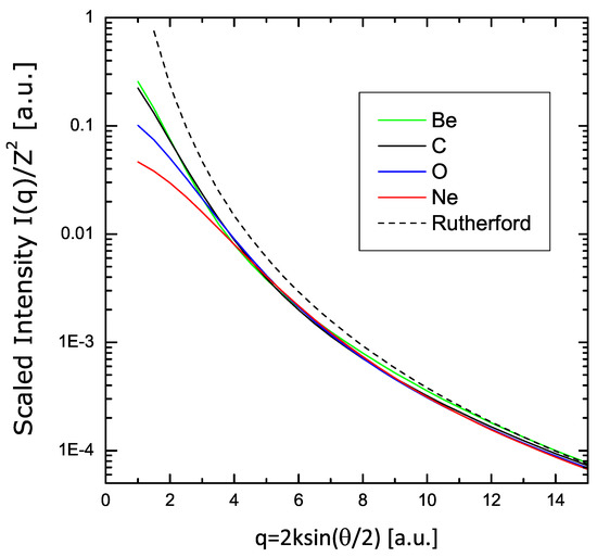
Figure 8.
Scaling of the scattering intensity using the same calculations of Figure 7, plotted here in form , showing the asymptotic convergence to the Rutherford limit .
7.2. Plasma Stopping Power
The standard expression for the stopping power of a medium with dielectric function incorporating the ion form factor was given in Refs. [37,38],
Here, I will apply this formulation to a plasma with Tokamak-like conditions, namely: density cm and temperature K, using the classical dielectric function with a quantum cut-off from Ref. [39].
The results for C and Ne ions with charge states 0, 2+, and 4+ are shown in Figure 9 and Figure 10. The lines in these figures are the results of the variational model (V2), while the circles are similar calculations using the HF form factors. Again, an excellent agreement is obtained.
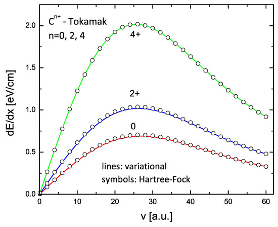
Figure 9.
Energy loss of carbon in a Tokamak plasma with density cm and temperature K for three charge states: 0, 2+, and 4+. The lines are the calculations using variational form factors (two-parameter formulation); the circles are the calculations using HF form factors.
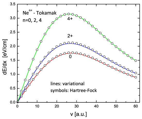
Figure 10.
Same as in Figure 9 but for , , and .
These comparisons, as well as the previous ones, show the convenience of using the variational method to obtain reliable values of scattering intensities (for high-energy electrons) and of the energy loss of ions in plasmas for the whole set of ions covered by this study. It may be expected that similarly good results could be obtained in other processes of interactions of ions or ion beams with matter.
8. Summary and Conclusions
In this work, an extension of the variational approach for atomic systems has been made in a way that applies to all the atoms and ions with atomic numbers up to 10. This includes a total of 45 cases (not considering the trivial cases where ). The approach considers two alternative formulations in terms of one- and two-variational parameters. The most complicated part of this work has been the calculation of numerous electron-interaction integrals. All these integrals have been calculated analytically, as described in Appendix A, obtaining exact algebraic results for the one- and two-parameter formulations given in Appendix B.
In the one-parameter description, the value of the variational parameter was calculated exactly. In the two-parameter case, the values of the parameters were obtained numerically using the exact algebraic expressions for the variational energy.
The results of these calculations are presented in two tables that include all the atoms and ions in the range of this study.
From the theoretical point of view, the extension of the variational method to a larger group of ions and atoms fills a long-standing gap in this area.
Although the present calculations were cumbersome due to numerous electron interactions that were involved, the application of the results should be quite straightforward using the tabulated values of parameters together with the remarkably simple expression of the form factor given by Equations (40)–(43). This makes the formulation specially useful for the handling of complex problems.
The comparisons with Hartree–Fock calculations show distinct views: while significant differences are found for the electron densities, the results of form factors show fairly good agreements in the one-parameter description and excellent agreements when two variational parameters are used. The comparison of total energies is also in excellent agreement with HF values.
This opens the way to a number of applications in different areas of research. Two examples were considered in this work: elastic scattering of high-energy electrons by atoms and energy loss of C and Ne ions in Tokamak plasmas. In both cases, the results of the variational approach were in excellent agreement with HF calculations. These examples serve as brief illustrations of the possibilities of the variational approach to replace with a good level of accuracy some of the most sophisticated calculations made on the basis of the Hartree–Fock method. It is indeed quite remarkable that the variational formulation using only two parameters gives results that compare so well with those of the HF theory, which requires 26 parameters for each atom or ion.
Some of the contexts in which the present variational approach may be useful include the area of current nuclear fusion studies (both in the lines of magnetically confined and inertially confined plasmas), as well as in space science or in cases of astrophysical interest, such as processes involving highly ionized elements in stellar interiors. Still, other possible areas of application are the area of medical physics, where irradiation with high-energy ion beams plays a very important role or in technological applications using ion beams. The convenience of a simplified but still fairly accurate method may become a very useful alternative in these areas, particularly in computer codes to simulate large or complex systems.
Finally, it is interesting to notice that the analysis performed here may be applied as well to ions with atomic numbers when the state of ionization is such that the number of remaining bound electrons is in the range 1–10. Thus, for instance, ions of with , or with can also be described through this formulation (with appropriate values of the variational parameters). Therefore, the number of ions to which this formulation applies is actually much larger than the cases considered in this work.
Funding
This research received no external funding.
Data Availability Statement
Not applicable.
Conflicts of Interest
The author declare no conflict of interest.
Appendix A. Calculation of Interaction-Energy Terms
The calculation of direct and exchange interaction terms is made using Equations (24)–(27). A large number of interactions appear when the number of electrons increases; a total of 22 different integrals have been calculated, considering the one-parameter and the two-parameter cases. All the integrals were calculated analytically, obtaining exact algebraic values. I will give here a brief summary of the calculation procedures with a few illustrative examples. The complete set of results is contained in Appendix B.
Appendix A.1. Direct Interactions
- (1)
- Terms , , and :
The treatment of the integrals for the case is rather elementary and has been described in textbooks. Due to the spherical symmetry, a very similar treatment can be applied to the integrals corresponding to the and interactions. These integrals have been evaluated in Ref. [32]. Therefore, I will skip these cases and will go directly to the treatment of the integrals that involve orbitals. Here I just write the results for the former cases:
- (2)
- Calculation of terms and :
From symmetry considerations (since the and densities are spherically symmetric), it may be shown that the interaction energies are independent of the orientation of the orbitals; therefore, they are the same for the and states. In particular, I will consider here the interaction between the and the orbitals given by
Using the representation of in terms of spherical harmonics given by Equation (26), and separating the radial and angular terms of , as in Equation (15), the angular integration derives in terms of the form
where:
where I have used the relation:
Therefore, the angular integral becomes
Then, the sum of spherical harmonics in the expression of reduces to the term , , and (considering the factor = , for ) the radial integral separates into the following two terms:
and
where is the function defined by Equation (17).
The calculation of these two integrals, in the simplest case of the one-parameter formulation, yields (in atomic units)
A fully similar calculation can be made for the case, with the only difference of changing by in the radial integrals. The result, also for the one-parameter case, is
The calculations for the two-parameter cases are much more cumbersome and yield rather awkward results given in Appendix B, Equations (B14)–(B18).
- (3)
- Cases :This comprises three cases: , , and , which give different results, since the spatial overlap of the corresponding densities are different. The calculations for these cases are as follows.
- (3a)
- Term :Using the function defined before, the interaction-energy integral isIn this case, the two angular integrals are equal,Then, the angular integration now provides two terms:This leads to the energy expressionAgain, this may be separated into two integrals (with and ), leading to the final result
- (3b)
- Term :Consider now the second case Using the function defined before, the energy integral isThe angular integrations may be performed using Equation (A8) andwhich leads to:which again may be split into the corresponding integrals for and .The integrations are rather long but straightforward and yield the final result:
- (3c)
- Term :The integrals for the cases , , and are equal. Considering the case, the integral becomesand after angular integrations, we getSeparating the integrals for the cases and as before and performing these integrations, one obtains the final result:
Appendix A.2. Exchange Interactions
The calculation of the exchange integrals is similar to the previous ones but still more tedious. I will show here two particularly interesting examples.
- (i)
- case:
From Equation (25), the corresponding integral in this case is
The angular dependence of is
with
(where ).
Using the expansion of in spherical harmonics, the angular integrals are now:
and the corresponding factor in the expansion is
Then, we obtain the and contributions:
The radial integrations are now more complicated due to an entanglement of the parameters and , and at the end, one obtains
In the one-parameter case, this reduces to:
- (ii)
- case:
The form of the exchange integral here is
and using the wave functions from Section 2.1 (Equations (11) and (12)) and the auxiliary function , the integral takes the form
(with ), where represents the angular integration
Using the expansion of in terms of spherical harmonics, we get the terms of the angular integration:
and
Using the property
we finally get
The corresponding factor in the expansion is now , and the radial integrals for and take the form:
Evaluating these integrals with the function of Equation (A28) I finally get
Appendix B. Values of Direct and Exchange Integrals
The calculation of the direct and exchange integrals was made according to the procedures exemplified in Appendix A. This appendix contains the results of calculations of all the integrals for the one-parameter and two-parameter cases.
Appendix B.1. One-Parameter Case
- (i)
- Direct/Coulomb integrals
The exact algebraic results and numerical values of all the electron–electron interaction energies are the following (values given in atomic units):
:
:
:
:
:
:
:
:
- (ii)
- Exchange integrals
The values of the terms corresponding to exchange energies are the following:
1s − 2s:
1s − 2p:
2s − 2p:
:
:
I wish to notice that the results for the terms 1s − 1s, 1s − 2s, and 2s − 2s agree with those obtained earlier by Kaneko [32].
Appendix B.2. Two-Parameter Case
The integrals for the two-parameter case can be handled in similar ways, as discussed in Appendix A, but the calculations of the double integrals become much more cumbersome due to the entanglement between the parameters and when the s and p orbitals are combined. Here, I give the corresponding results.
The terms corresponding to interactions between and electrons are the same as given in Equations (B1)–(B3) and (B9) since they involve only the single parameter Therefore, I write here only the new terms related to orbitals (including the interactions between the s and p orbitals).
- (i)
- Direct/Coulomb integrals
The interaction between the and orbitals may be expressed as:
where:
The interaction between the and orbitals contains two terms:
where:
The other three integrals depend only on parameter ,
- (ii)
- Exchange integrals:
The exchange integral between and states is the same as in Equation (B9), in terms of parameter . The additional exchange terms involving states are the following:
This completes the whole set of cases that must be taken into account for the analysis of the electronic structure of atoms and ions considered in this work.
Appendix B.3. Example: Expressions for the Variational Energy
For the sake of clarity and for further applications, it is useful to give an example of how the expressions for the variational energy are constructed. Here I will show the case of Neon, which contains all the energy terms quoted before, and implicitly contains all the possible cases of atoms or ions considered in this study.
As discussed in the text, from the knowledge of these expressions, one can obtain the expressions for all the atoms and ions with by considering the equivalence of electronic structures provided by the isoelectronic considerations mentioned in the text. Therefore, the energy expression for any other ion or atom is formally the same as the one for the ion that contains the same number of electrons as the particular ion or atom being considered (but the values of the variational parameters will be different).
As indicated in the main text, I have used letters U, V, and W to represent the three types of interaction terms: electron–nucleus interactions (U), direct (V), and exchange (W) interactions between electrons.
First, I write the expression for the energy of the atom, namely:
Then, the energy of the atom is expressed in terms of that of as follows:
where
In the same way, the energy of is written as in Equation (B27), where now
With the same criterion, the energies of the following ionization states of are given by the following expressions of :
For :
For :
For :
For :
For the following charge states, since there are no p electrons. Therefore, we can write the energy of the ion as:
Notice that this expression is the same as the one for but with a different value of the nuclear charge ( instead of 4) in the electron–nucleus interactions and .
Similarly, the energy of the ion contains the same terms as (with Z=10 instead of 4) and is given by
and the energy of , which contains the same terms as , or , reduces to
Finally, the cases of (hydrogen-like) and (bare nucleus) are trivial.
References
- Herzberg, G. Atomic Spectra and Atomic Structure; Dover Publications: New York, NY, USA, 1944. [Google Scholar]
- Hartree, D.R. The Calculation of Atomic Structures; John Wiley and Sons: New York, NY, USA, 1957. [Google Scholar]
- Condon, E.U.; Shortley, G.H. The Theory of Atomic Spectra; Cambridge University Press: London, UK, 1959. [Google Scholar]
- Slater, J.C. Quantum Theory of Atomic Structure; McGraw-Hill: New York, NY, USA, 1960. [Google Scholar]
- Bethe, H.A.; Jackiw, R. Intermediate Quantum Mechanics; W.A. Benjamin: New York, NY, USA, 1968. [Google Scholar]
- Bransden, B.H.; Joachain, C.J. Physics of Atoms and Molecules; Longman Group UK: Essex, UK, 1983. [Google Scholar]
- Kastberg, A. Structure of Multielectron Atoms; Springer: Berlin/Heidelberg, Germany, 2020. [Google Scholar]
- Bethe, H.A.; Salpeter, E.E. Quantum Mechanics of One- and Two-Electron Atoms; Plenum Publishing: New York, NY, USA, 1977. [Google Scholar]
- Gombás, P. Die Statistische Theorie des Atoms und Ihre Anwendungen; Springer: Vienna, Austria, 1949. [Google Scholar]
- March, N.H. Self-Consistent Fields in Atoms; Pergamon: New York, NY, USA, 1975. [Google Scholar]
- Spruch, L. Pedagogic notes on Thomas-Fermi theory (and some improvements): Atoms, stars, and the stability of bulk matter. Rev. Mod. Phys. 1991, 63, 151. [Google Scholar] [CrossRef]
- Clementi, E.; Roetti, C. Roothaan-Hartree-Fock Atomic Wavefunctions. At. Data Nucl. Data Tables 1974, 14, 177. [Google Scholar] [CrossRef]
- Shevelko, V.P.; Vainshtein, L.A. Atomic Physics for Hot Plasmas; Institute of Physics: London, UK, 1993. [Google Scholar]
- de Michelis, C.; Mattioli, M. Spectroscopy and impurity behaviour in fusion plasmas. Rep. Prog. Phys. 1984, 47, 1233. [Google Scholar] [CrossRef]
- Mehlhorn, T.A. A finite material temperature model for ion energy deposition in ion driven inertial confinement fusion targets. J. Appl. Phys. 1981, 52, 6522. [Google Scholar] [CrossRef]
- Miškovic, Z.; Wang, Y.-N.; Song, Y.-H. Dynamics of fast molecular ions in solid and plasmas: A review of recent theoretical developments. Nucl. Instrum. Methods Phys. Res. Sect. B 2007, 256, 57. [Google Scholar] [CrossRef]
- Barriga-Carrasco, M.D. Heavy ions charge-state distribution effects on energy loss in plasmas. Phys. Rev. E 2013, 88, 043107. [Google Scholar] [CrossRef]
- Clauser, C.F.; Farengo, R. Alpha particles diffusion due to charge changes. Phys. Plasmas 2015, 22, 122502. [Google Scholar] [CrossRef]
- Clauser, C.F.; Farengo, R. The effect of inelastic collisions on the transport of alpha particles in ITER-like plasmas. Nucl. Fusion 2017, 57, 046013. [Google Scholar] [CrossRef]
- Kawata, S.; Karino, T.; Ogoyski, A.I. Review of heavy-ion inertial fusion physics. Matter Radiat. Extrem. 2016, 1, 89. [Google Scholar] [CrossRef]
- Archubi, C.D.; Arista, N.R. Unified description of interactions and energy loss of particles in dense matter and plasmas. Phys. Rev. A 2020, 102, 052811. [Google Scholar] [CrossRef]
- Lifschitz, A.; Sylla, F.; Kahaly, S.; Flacco, A.; Veltcheva, M.; Sanchez-Arriaga, G.; Lefebvre, E.; Malka, V. Ion acceleration in underdense plasmas by ultra-short laser pulses. New J. Phys. 2014, 16, 033031. [Google Scholar] [CrossRef]
- Hansen, C.J.; Kawaler, S.D.; Trimble, V. Stellar Interiors, Physical Principles, Structure, and Evolution; Springer: New York, NY, USA, 2004. [Google Scholar]
- Reeves, H. Stellar Evolution and Nucleo-Synthesis; Gordon and Breach: Philadelphia, PA, USA, 1968. [Google Scholar]
- Clayton, D. Principles of Stellar Evolution and Nucleosynthesis; University of Chicago Press: Chicago, IL, USA, 1984. [Google Scholar]
- Durante, M.; Cucinotta, F.A. Physical basis of radiation protection in space travel. Rev. Mod. Phys. 2011, 83, 1245. [Google Scholar] [CrossRef]
- Schardt, D.; Elsasser, T.; Schulz-Ertner, D. Heavy-ion tumor therapy: Physical and radiobiological benefits. Rev. Mod. Phys. 2010, 82, 383. [Google Scholar] [CrossRef]
- Paul, H. On the accuracy of stopping power codes and ion ranges used for hadron therapy. Adv. Quantum Chem. 2013, 65, 39. [Google Scholar]
- Vera, P.D.; Garcia-Molina, R.; Abril, I.; Solovyov, A.V. Semiempirical Model for the Ion Impact Ionization of Complex Biological Media. Phys. Rev. Lett. 2013, 110, 148104. [Google Scholar] [CrossRef]
- de Vera, P.; Taioli, S.; Trevisanutto, P.E.; Dapor, M.; Abril, I.; Simonucci, S.; Garcia-Molina, R. Energy Deposition around Swift Carbon-Ion Tracks in Liquid Water. Int. J. Mol. Sci. 2022, 23, 6121. [Google Scholar] [CrossRef] [PubMed]
- Flügge, S. Practical Quantum Mechanics; Springer: Berlin/Heidelberg, Germany, 1994. [Google Scholar]
- Kaneko, T. Energy loss of swfit projectiles con n (n ≤ 4) electrons. Phys. Rev. A 1994, 49, 2681. [Google Scholar] [CrossRef]
- Jackson, J.D. Classical Electrodynamics; Wiley: New York, NY, USA, 1962. [Google Scholar]
- Brandt, W.; Kitagawa, M. Effective stopping-power charges of swift ions in condensed matter. Phys. Rev. B 1982, 25, 5631. [Google Scholar] [CrossRef]
- Mathar, R.J.; Posselt, M. Effective-charge theory for the electronic stopping of heavy ions in solids: Stripping criteria and target-electron models. Phys. Rev. B 1995, 51, 107. [Google Scholar] [CrossRef]
- Mott, N.F.; Massey, H.S.W. The Theory of Atomic Collisions; Oxford University Press: London, UK, 1950. [Google Scholar]
- Ferrell, T.L.; Ritchie, R.H. Energy losses by slow ions and atoms to electronic excitations in solids. Phys. Rev. B 1977, 16, 115. [Google Scholar] [CrossRef]
- Echenique, P.M.; Flores, F.; Ritchie, R.H. Dynamic Screening of Ions in Condensed Matter. Solid State Phys. 1990, 43, 229. [Google Scholar]
- Peter, T.; Meyer-ter-Vehn, J. Energy loss of heavy ions in dense plasma. Linear and nonlinear Vlasov theory for the stopping power. Phys. Rev. A 1991, 43, 1998. [Google Scholar] [CrossRef] [PubMed]


Disclaimer/Publisher’s Note: The statements, opinions and data contained in all publications are solely those of the individual author(s) and contributor(s) and not of MDPI and/or the editor(s). MDPI and/or the editor(s) disclaim responsibility for any injury to people or property resulting from any ideas, methods, instructions or products referred to in the content. |
© 2023 by the author. Licensee MDPI, Basel, Switzerland. This article is an open access article distributed under the terms and conditions of the Creative Commons Attribution (CC BY) license (https://creativecommons.org/licenses/by/4.0/).