Article

Applications of Machine Learning and Neural Networks for FT-ICR Mass Measurements with SIPT

1
Department of Physics and Astronomy, Michigan State University, East Lansing, MI 48824, USA
2
Facility for Rare Isotope Beams, Michigan State University, East Lansing, MI 48824, USA
3
Department of Chemical Engineering and Materials Science, Michigan State University, East Lansing, MI 48824, USA
*
Author to whom correspondence should be addressed.
Atoms 2023, 11(10), 126; https://doi.org/10.3390/atoms11100126
Submission received: 12 August 2023 / Revised: 10 September 2023 / Accepted: 22 September 2023 / Published: 28 September 2023
(This article belongs to the Special Issue Advances in Ion Trapping of Radioactive Ions)

Abstract

:
The single-ion Penning trap (SIPT) at the Low-Energy Beam Ion Trapping Facility has been developed to perform precision Penning trap mass measurements of single ions, ideal for the study of exotic nuclei available only at low rates at the Facility for Rare Isotope Beams (FRIB). Single-ion signals are very weak—especially if the ion is singly charged—and the few meaningful ion signals must be disentangled from an often larger noise background. A useful approach for simulating Fourier transform ion cyclotron resonance signals is outlined and shown to be equivalent to the established yet computationally intense method. Applications of supervised machine learning algorithms for classifying background signals are discussed, and their accuracies are shown to be ≈65% for the weakest signals of interest to SIPT. Additionally, a deep neural network capable of accurately predicting important characteristics of the ions observed by their image charge signal is discussed. Signal classification on an experimental noise dataset was shown to have a false-positive classification rate of 10.5%, and 3.5% following additional filtering. The application of the deep neural network to an experimental 85Rb+ dataset is presented, suggesting that SIPT is sensitive to single-ion signals. Lastly, the implications for future experiments are discussed.

1. Introduction

Precision nuclear mass measurements are fundamental quantities needed in practically every area of nuclear physics research. The masses of rare isotopes far beyond the valley of stability are of particular importance for both nuclear structure and astrophysics calculations [1,2,3,4,5]. Such measurements can be used to extract a large range of nuclear structure information, including shell structure, nuclear deformation, pairing, and effective interactions, among others. New accelerator facilities, such as the Facility for Rare Isotope Beams (FRIB), are expected to improve rare isotope production by orders of magnitude; however, many isotopes very far from stability would only be delivered at rates below ∼ 10 5  ions/s [6]—roughly one ion per day. The Low-Energy Beam Ion Trapping (LEBIT) facility at FRIB performs precision mass measurements of these isotopes using Penning trap mass spectrometry—the most precise method known to date [7,8]. Techniques such as time-of-flight ion cyclotron resonance (TOF-ICR) [9] and phase-imaging ion cyclotron resonance (PI-ICR) [10], while flexible, are destructive and require hundreds of ions to complete a mass measurement. Measuring mass information to the needed precision for shell structure evolution [11,12] away from stability is difficult and often infeasible given the low delivery rates of the isotopes of interest, particularly near the doubly magic 100Sn and 78Ni which are of current interest.
The single-ion Penning trap (SIPT) developed by LEBIT addresses these shortcomings with the narrowband Fourier transform ion cyclotron resonance (FT-ICR) technique [13]. SIPT has been developed specifically to achieve the needed mass precision for single isotopes, which are of high importance to nuclear structure and astrophysics studies. This technique is suited to low delivery rates, as a measurement relies only on recording the image current produced by ions in the trap. This is of particular use for the most exotic rare isotopes, such as those near the proton/neutron drip lines. FT-ICR measurements can be performed with only a single ion given a suitably low-noise amplification circuit. The challenge in performing these measurements is that the weak ion signals and electronic noise are often comparable and can be easily conflated. Various measured and simulated cases are presented in Figure 1, illustrating the difficulty associated with this problem.
The classification of these signals as either background or from ions is a problem well suited to supervised machine learning techniques [14,15]. Caution is often required when utilizing machine learning as the models are limited in parameter scope and are susceptible to over-fitting a trend to data. As such, stable numerical approaches should always be favored when possible. This is not easily feasible for the problem at hand: cases where ion signals and noise have comparable amplitudes become exceptionally difficult to ‘fit’, if not impossible. Machine learning is applied as a means of extracting as much information from each signal as possible, with the understanding that predictions are probabilistic.
Machine learning algorithms use a large set of labeled data to predict the most likely classification for an unknown instance. Machine learning, including deep neural networks, has recently been applied to a variety of nuclear physics problems such as determining nuclear mass [16,17], nuclear charge radius [18], and ground-state energy [19], among many others. Applications of machine learning for FT-ICR mass measurements have been explored, but tend to focus on sample analysis such as biomarker profiling [20,21], accounting for space charge effects [22,23], or molecular mass spectrometry [24]. These applications are of no particular significance to precision isotope mass measurements with SIPT. No previous work could be identified addressing the classification of background signals using machine learning on FT-ICR data, or for determining ion characteristics in an FT-ICR Penning trap.
In this paper, several machine learning models are presented which are used to identify ion signals from electronic noise and extract important characteristics of ions within the detector. The necessary background regarding the mass measurement technique, theoretical models, and the specifics of the SIPT detector is presented in Section 2. A method for efficiently simulating realistic SIPT FT-ICR signals is discussed in Section 3. Section 4 highlights the procedure for applying supervised machine learning algorithms for signal vs. noise classification. In Section 5, a deep neural network (DNN) predicts ion characteristics for a large set of measured isotope signals in SIPT. Section 6 applies the classification algorithms to an experimental dataset and estimates the characteristics of the ions using the neural network. Conclusions and directions for future work are provided in Section 7.

2. Background

2.1. Ion Motion in a Penning Trap

Using Penning traps for ion capture and excitation is well established [8], and a brief summary is presented here for context. A Penning trap uses a homogeneous magnetic field and a quadrupolar electrostatic field which confines charged particles in space. Mass measurements are made possible through the determination of the characteristic cyclotron frequency of a trapped ion. This frequency is related to the ion’s mass by
ω c = 2 π ν c = q B m
where q and m are the ion charge and mass, respectively, and B is the magnetic field strength. This ion motion is a superposition of an axial motion (defined as the z-direction and parallel to the magnetic field) with frequency
ω z = 2 π ν z = q U 0 m d 2
and two radial motions with frequencies
ω ± = 2 π ν ± = ω c 2 ± ω c 2 4 ω z 2 2
where U 0 is the potential difference between the endcap and ring electrodes, and d is a characteristic trap parameter. Furthermore, the eigenfrequencies satisfy the following relationship:
ω c =   ω + + ω .
The position of an ion in the trap is described by the following equations:
x =   ρ + cos ( ω + t + ϕ + , 0 ) + ρ cos ( ω t + ϕ , 0 ) y =   ρ + sin ( ω + t + ϕ + , 0 ) + ρ sin ( ω t + ϕ , 0 ) z =   ρ z cos ( ω z t + ϕ z , 0 )
where ρ ± , ϕ ± , 0 and ρ z , ϕ z , 0 are the radial amplitudes and initial phases of the radial and axial eigenmotions. Dipole and quadrupole radio frequency (RF) excitations can be applied to the Penning trap to modify and convert between ρ + and ρ ; further specifics are discussed in [9]. The application of these excitations also impacts the eigenmotion phases, ϕ ± , 0 , and a derivation of this effect is presented in [25]. Notably, for multiple ions in the trap, longer RF dipole excitations of ρ ± correspond to a tightening of the distribution of ϕ ± such that the relative ion spatial distribution remains constant regardless of excitation time. The effect of a sufficiently long dipole excitation is observed by the center of the ion ‘spot’ moving to a larger radius while the shape of the spot remains unchanged.

2.2. Fourier Transform Ion Cyclotron Resonance Technique

The non-destructive narrowband Fourier transform ion cyclotron resonance (FT-ICR) technique used by SIPT is sensitive to the image current on the Penning trap ring electrode segments, produced as ions undergo their characteristic eigenmotions [13]. A narrowband approach limits the observable frequency range to be near that of the eigenmotion being probed for a given isotope [26]. The resulting image current signal is a combination of noise as well as contributions from each ion present in the trap. This signal is very weak—typically of the order of femtoamperes—and requires further amplification to be readable. SIPT uses a low-noise, high-quality factor resonator circuit sufficient for detecting the image charge of a singly charged ion. Both the SIPT and detection circuit are operated at cryogenic temperatures to further reduce thermal noise, improving the signal-to-noise ratio of the detected ion signals by a factor of eight compared to room temperatures. A discrete Fourier transform (DFT) [27] is then applied to the time-domain signal to produce the frequency spectrum, from which the eigenfrequency of interest can be identified. Often, this is achieved by fitting a peak in the frequency spectrum to a characteristic Lorentzian curve of the form
L ( ν ) = L 0 + | b | · c ( ν ν 0 ) 2 + c 2
where L 0 is an initial offset, b and c are the characteristic height and width, respectively, and ν 0 is the distribution center. In this formulation, the total area of the distribution is b π . Since the eigenfrequency is expected at the peak value, ν 0 , one can determine the isotope’s mass from Equations (1) and (4).
The ion image current signal is directly proportional to the ion’s charge: FT-ICR is increasingly more sensitive for multiply charged ions [13]. This poses an even greater challenge for measurements of a single singly charged ion. Given the negative impact of noise on the potential resolving power, the ability to identify, isolate, and filter noise is highly desirable. This problem has been the subject of various studies [28,29,30,31], and various FT-ICR techniques have been developed to improve the signal-to-noise ratio achievable [32,33,34]. However, these techniques are not suited to the narrowband FT-ICR technique, or have limited applicability for precision mass measurements of rare or exotic nuclei. Furthermore, selective noise filtering techniques are not effective for the typically weak SIPT ion signals as they can be significantly distorted.
The FT-ICR signal strength for a given eigenmotion(s) is also highly dependent on which of the segmented ring electrodes in the Penning trap are used for detection or excitation [35,36]. Often this detection scheme is chosen to maximize the signal amplitude of the eigenfrequency being probed. Simulations were performed in [36] to determine an optimal configuration of detection/excitation electrodes for cyclotron and reduced cyclotron frequency pickup. In [35], simultaneous detection of ω c and ω + using a single detection circuit was demonstrated, which provides an unambiguous ion signature if both frequencies are observed. However, this method is still in development for SIPT and would also require frequency identification in two separate regions. For these reasons, the measurements discussed in this work consider the established dipole pickup of only the modified cyclotron frequency ν + , whose scheme is illustrated in Figure 2.
Ion motion in the Penning trap also plays an important role in the achievable signal strengths. As discussed in Section 2.1, the phase distribution of ions following a dipole RF excitation converges for longer excitation times. This is of critical importance for FT-ICR measurements as each signal is a superposition of all ion image current signals. As such, for multiple ions, destructive interference of the ion image current signals can occur, even more so if the phase distribution spans a large range. A large phase distribution is not always avoidable, and is limited in part by the injection of ions into the Penning trap: reduced cyclotron motion is introduced as ions cross magnetic field lines due to imperfect alignment. Longer duration dipole RF excitations cannot always be used to reduce the phase spread as electric field imperfections are amplified at larger radii [9]. An additional consideration is the impact of axial motion introduced by non-optimal ion injection into the Penning trap. Realistic simulations of FT-ICR signals, such as the one presented in Section 3.3, suggest that axial oscillations in SIPT have a negligible impact (∼ 1 part in 10 5 for ρ z 0.25 ρ + ) on the eigenfrequency signal strength, and as such are not considered further for this work.

3. Numerical Simulation

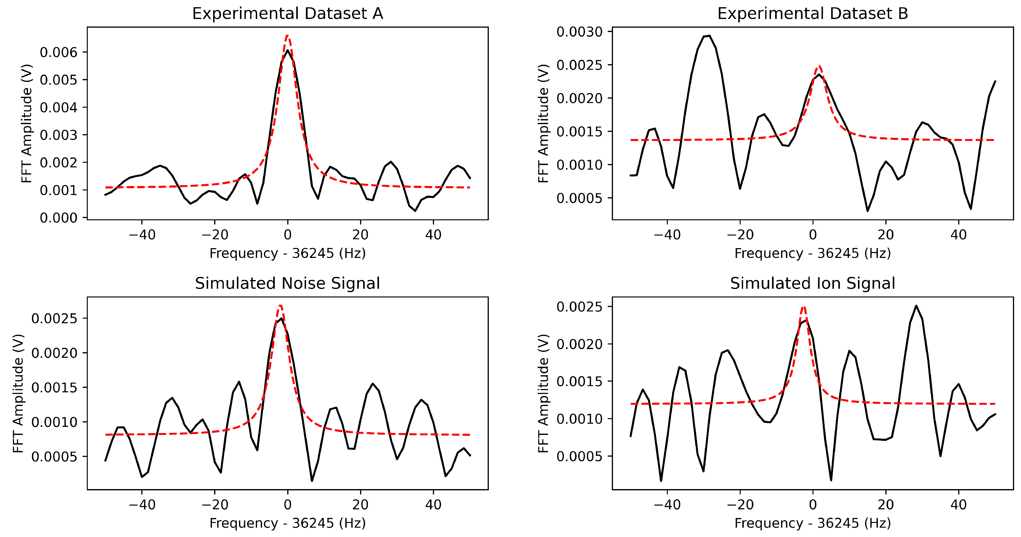
3.1. Noise Floor Determination

Considering a realistic construction of the SIPT detector noise floor, the dominant source of noise in FT-ICR signals is expected to be root mean-squared (RMS) Johnson–Nyquist noise [37]. Assuming an ideal resistor, RMS noise is approximately white [38]. The broadband noise power spectral density (PSD) of an FT-ICR detection circuit, however, is generally not white, since it is subject to resonances from the RLC amplifier and other external sources. The narrowband FT-ICR measurements used by SIPT focus on a small frequency band around the eigenfrequency being probed. Within a sufficiently narrow band, noise can be reasonably approximated as white. A model for the simulated noise signal at any point in time is defined simply as
S noise ( t ) = U ( 0 , A noise )
where U denotes the uniform random distribution from zero to a maximum of A noise . Measured background signals from SIPT can then be compared to a simulated noise signal of the same length by their power spectral densities (PSDs). When determining the PSD, a spectral bandwidth of 100 Hz centered about the expected ion frequency was used, as it captures the maximum expected width of the ion signals by at least a factor of ten. Comparisons of the average PSDs for a large set of both simulated and measured noise signals are shown in Figure 3. A reasonable white noise approximation with an amplitude of A noise 4.85  mV was determined to best fit the measured background noise power from SIPT.

3.2. Simulated Signal-to-Noise Ratio

The signal-to-noise ratio (SNR) is a useful metric for quantifying the strength of a desired signal to that of the intrinsic noise. The ability to accurately identify weak signals is directly related to this ratio: an ion signal with a larger SNR becomes more clearly defined from noise. A general definition for the signal-to-noise ratio is
SNR = P signal P noise
where P signal ,   noise are the powers of the signal and noise, respectively. The power for either the signal or noise is calculated as the integrated Fourier spectrum over a finite spectral bandwidth. In the case of simulated data, the SNR can be determined in this manner since both the noise and ion signal are known independently.
For an FT-ICR Penning trap, assuming RMS Johnson–Nyquist noise, the signal-to-noise ratio (SNR) is approximated by
SNR = κ π 4 N q e ρ ρ 0 ν Δ ν Q k B T C
where κ 0.93 is a geometrical parameter that accounts for the fact that the pickup electrodes are not infinite flat planes; N is the number of ions; q e is the ion charge; ρ / ρ 0 is the radius of the ions’ orbit relative to the trap radius; ν / Δ ν is the ratio of the ion eigenfrequency to the spectral bandwidth; k B is the Boltzmann constant; and Q, T, and C are the quality factor, temperature, and capacitance of the detection circuit, respectively [7,39]. Maximizing the quality factor of the RLC resonator is essential to achieving reasonable SNR values for single-ion signals, and a baseline of Q 1000 is necessary. For the SIPT, typical values for these parameters are ρ / ρ 0 0.5 , Q = 2785 , T = 5  K, and C 30  pF. The capacitance of the resonator is tuned for a given isotope such that the SIPT resonator peaks at the eigenfrequency being measured. Lastly, the radius of the ion in the trap is dependent upon the duration of the initial dipole excitation of the isotope eigenmotion. For single ions of 100Sn+ and 78Ni+, SIPT is expected to achieve SNR’s of roughly 5.5 / Δ ν   Hz 1 / 2 . The spectral bandwidth is left undetermined as it is limited by the measurement sample rate and acquisition time. A more precise measurement will yield a narrower resonance for the eigenfrequency being probed, which improves the SNR as a narrower spectral bandwidth can be used.

3.3. Methods for Simulating FT-ICR Signals

A rigorous method to simulate the image current of an ion undergoing cyclotron motion for a given Penning trap ring electrode configuration has been previously established [9], and a brief summary is presented here for completeness. The voltage readout of the ion image charge current on the Penning trap ring electrodes is given by
S ( t ) = R eff q v ( t ) · E 1
where R eff is the effective resistance of the detector circuit, which is dependent on the intrinsic resonator frequency; q and v ( t ) are the ion charge and velocity, respectively; and E 1 = E / V is the unit electric field generated by a ± 1  V potential difference applied to the detection electrodes. A discrete approximation of the electric field can be computed using SIMION [40] for the desired pickup scheme of the Penning trap ring electrodes. The ion velocity is found easily by differentiating the equations for ion position in Equation (5).
However, this method is computationally intensive as the fields must be determined for the ion at each new position. This becomes problematic for the machine learning algorithms used later in this work as they rely on a large dataset of these signals to adequately encompass the problem complexity. For example, the neural network in Section 5 requires the simulation of ∼ 10 8 unique ion signals to achieve an acceptable accuracy. It was estimated that approximately 200 days of calculation time using 64 fully dedicated CPUs would be required to complete all the required simulations on a state-of-the-art high-performance computing farm. Clearly, a faster simulation method is highly desirable. Given the expected periodic behavior of the signals, a simplified construction is used, where each ion’s image current is sinusoidal and acts independently. The overall voltage signal from all ions is simply a superposition of each ion’s contribution:
S ( t ) = S noise ( t ) + i = 1 N A i sin 2 π t f i + ϕ i
where N is the number of ions composing the signal; S noise is the signal contribution from noise; and A i , f i , and ϕ i are the amplitude, frequency, and initial phase, respectively, of the i th ion. This approach lends itself well to vectorization and is, thus, significantly faster (approximately 50 times faster than the rigorous method).
The general sum-of-sines algorithm is detailed in Algorithm 1. Each ion has its eigenfrequency selected from a normal distribution with a standard deviation of 0.5  Hz. This well encompasses the observed experimental uncertainty. Similarly, the voltage signal amplitude for a given ion is also selected from a normal distribution with a typical standard deviation of 0.005  mV. This approximates the beam spot radial distribution. The noise contribution to the signal is modeled by Equation (7) with A noise = 4.85  mV. Lastly, the phase spread, ϕ i , discussed in Section 2.1, is also chosen from a uniformly random distribution with a maximum value of ϕ 0 , max . Each simulated time-domain signal is sampled over 24,000 points, each 5 μs apart, for a total duration of 120 ms. The simulated frequency-domain signal was then computed using a fast Fourier transform (FFT).   
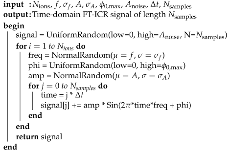
Algorithm 1: Serial method for simulating an FT-ICR time-domain signal using the ‘sum of sines’ approach. The inputs are as follows: N ions is the number of ions in the Penning trap; f and σ f define the ion eigenfrequency normal distribution; A and σ A define the single-ion amplitude normal distribution; ϕ 0 , max is the maximum eigenmotion phase; A noise is the noise amplitude; Δ t , N samples are the sample time and number of samples, respectively. The method UniformRandom (low, high, N = 1) samples N instances from a uniformly random distribution within the range defined from low (inclusive) to high (exclusive), and NormalRandom ( μ ,   σ ) randomly samples a Gaussian/normal distribution defined by a mean value μ and standard deviation σ .
Atoms 11 00126 i001
To compare the two methods and ensure the proposed method adequately approximates the more realistic SIMION approach, the SNR distributions for different numbers of ions in the Penning trap are analyzed for both approaches. Again, a spectral bandwidth of 100 Hz about the known eigenfrequency is used, capturing the width of expected ion signals by at least a factor of ten. The noise level of A noise = 4.85 mV determined in Section 3.1 is used. The relationship between the SNR and the ion position in the trap, ρ / ρ 0 for the rigorous method, and SNR to the single-ion signal amplitude, A single for the sum-of-sines approach, were determined at a 95% confidence level as
SNR =   0.229673 ( 13 ) ρ ρ 0
SNR =   9.896849 ( 3 ) [ mV 1 ] A single
where both have offsets compatible with zero, and the SNR was determined over a 100 Hz spectral bandwidth. Using the expected SNR’s for 100Sn+ and 78Ni+, the approximate single-ion signal amplitude is A single ∼ 0.02 mV. This is used as a point of reference when determining a reasonable amplitude for 85Rb, for which a large dataset of signals have been collected. Furthermore, combining these relationships provides a correlation between the relative ion radius in the Penning trap to the simulated amplitude for a single ion:
ρ ρ 0 = 43.063 ( 2 ) [ mV 1 ] · A single
where the uncertainty is determined in quadrature at a 95% confidence level. A comparison of the signals generated from Equations (10) and (11) for equivalent SNR’s using Equation (14) and different phase spreads is presented in Figure 4.
Of primary interest is the relative positioning and widths of the distributions. The results are equivalent, so the approximation presented in Equation (11) is used for the remaining work.

4. Identification of Ion Signals

A reliable means of identifying ion signals, especially in cases with small signal-to-noise ratios, is fundamental to performing the mass measurement. Machine learning algorithms are well suited to this type of task. These algorithms (also known as models) require two sets of information: the ‘feature set’ (also known as model input) and a ‘prediction set’ (also known as model output). The feature set is the data provided to the algorithm upon which predictions are based on. A prediction set is the matching pair to the input that informs the algorithm of the true output. When training a machine learning model, a large dataset of known inputs and true outputs is used to optimize its algorithm in some fashion. The performance of each classifier is evaluated using its precision: the number of true-positive classifications relative to the true number of true-positive and false-positive instances. Precision was chosen as the cost of a false-positive classification (noise mistaken for an ion signal) is deemed greater than the cost of a false-negative classification (ion signal mistaken for noise) [41]. A standard means of evaluating the performance of a classifier is using cross-validation [42]. Specifically, k-fold cross-validation is used throughout this work to compare the precision between models.
For identification of ion signals, the model used is a ‘binary classifier’ which labels a given feature set as either noise or an ion signal. Four classifiers from the Scikit-learn library [43] are considered: k-nearest neighbors (kNN), Gaussian naive Bayes (GNB), support vector machine (SVM), and logistic regression (LR). These algorithms were chosen based on their performance and suitability for the frequency data used to make the classification. There are many other standard algorithms, like decision trees, linear regression, and neural networks. However, these methods showed no particular benefits, and initial investigations showed no performance increase over other models. These options were not considered further.

4.1. Dataset Construction for Signal Classifiers

The frequency spectra, relative to the expected ion frequency, of the SIPT signals are used for the classifier feature set. In principle, these should be independent of the frequency magnitude of the signal, allowing the classifier to be used for signals generated by ions of any mass. This assumes the noise remains white at any frequency magnitude, an assumption which is largely preserved for a narrow frequency band. The classifiers are dependent of the frequency resolution of the signals: this is limited by the sampling rate and total acquisition time of the signal. Signals with higher resolution, however, can easily be down-sampled to match the required frequency resolution of the classifier. The parallel nature of the signal model of Equation (11) allows for new training datasets to be quickly generated if needed. The work presented here considers time-domain signals with a total of 24,000 samples, each 5 μs apart, for a total time of 120 ms.
Including noise data at frequencies far beyond the expected ion frequency has the potential of ‘confusing’ classifiers, as such datapoints are ‘informationless’: a known concern for classifier reliability and efficiency [44,45]. Furthermore, the frequency resolution of the FFT allows signal peaks to be either clarified or obfuscated within the surrounding noise. Additional frequency granularity can be interpolated from an FFT by padding the time-domain signal with additional zeros. This process is referred to as zero-padding [46]. A zero-padding multiplier, α , was defined to mean appending α N t zeros to the time-domain signal of length N t . Beyond aiding classification, including further interpolated frequency information is also important for accurately fitting the spectrum to the characteristic Lorentzian curve. Minimal improvement was observed in classification performance beyond a padding multiplier of one to both the left and right ends of the signal. However, a minimum multiplier of two was observed to significantly improve the reliability of curve fitting.
Since the narrowband FT-ICR approach is used, the FFT spectrum is limited to a narrow range encompassing the expected ion eigenfrequency. A large frequency range is potentially important for generalizing noise trends, but this can also overshadow the importance of a valid ion peak. The optimal frequency range should then maximize the classifier performance while minimizing false-positive and false-negative classifications. An investigation of classification precision using a 10-fold cross-validation [47] approach with 10,000 samples, for different frequency ranges centered about ν c , is shown in Figure 5.
One pertinent feature is the stability of the classifiers across frequency ranges. A higher degree of stability suggests a robust determination of the relevant frequency information regardless of additional noise. All the classifiers display some level of instability for narrower frequency windows. Another important aspect to consider is that smaller frequency ranges increased the rate of false-positive classifications. This is likely due to an over-weighting of features near the expected eigenfrequency.
Taking these findings into consideration, the following method was devised. First, the time-domain signal for each simulated measurement was determined. After which, a zero-padding of twice the length the time-domain set was appended to both sides. Then, a fast Fourier transform was performed on the padded signal. Lastly, the frequency spectrum was reduced to only include frequencies within a 25 Hz window, centered at the expected eigenfrequency. In total, a set of 20,000 signals were generated for training and testing the accuracies of the classifiers.

4.2. Optimal Classifier Hyperparameters

For the classifiers of interest, choosing appropriate model hyperparameters is necessary to efficiently and accurately predict an unseen input. To accomplish this task in a systematic manner, a Bayesian optimization [48] approach is used. Specifically, the BayesSearchCV in the Python scikit-optimize [49] library is used for the primary hyperparameters for each classifier. A set of 10,000 simulated Fourier domain signals with an equal sampling of background and single-ion signals was used to train each model using a 5-fold cross-validation technique [47]. Initial ranges for hyperparameters in the optimization were chosen using a coarse grid over a large range of values and moving to a finer grid where clear positive trends were observed. In the case where multiple parameter sets were equivalently ranked, the set with the fastest training and prediction was chosen. A summary of the results for each classifier is presented in Table 1.

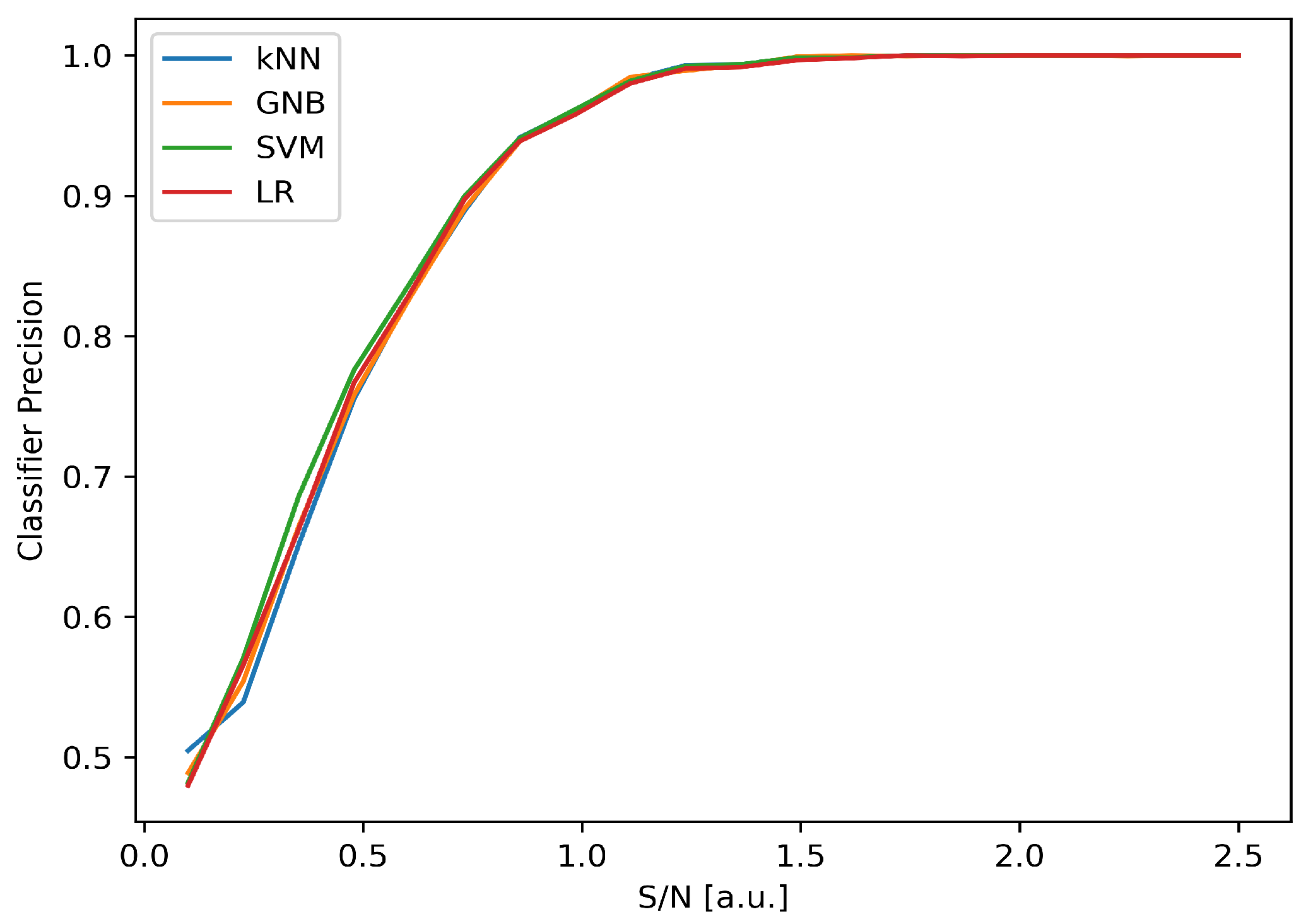
4.3. Classification of Ion Signals

A concern for experimental applications of these classifiers are mis-classifications, wherein noise propagates into the final mass calculation, or valid ion data are incorrectly identified as noise. This can be mitigated, in part, by a priori filtering of the signals. The simplest scheme would be to simply filter signals above a set SNR threshold which meets an acceptable false-positive classification rate. However, this is infeasible/inefficient for most single-ion measurements since they have signal amplitudes which can be on the order of the noise itself. A more intelligent scheme can be accomplished by first fitting a Lorentzian of Equation (6) to the frequency spectrum. Initial parameter values for this optimization are selected under the assumption of a valid ion signal, i.e., ν 0 = ν c , ± . The filtering scheme uses a priori knowledge of the ion being measured such that restrictions can be placed on the Lorentzian fit parameters. For example, requiring the fitted center frequency to be within a finite range of the expected cyclotron frequency, requiring the characteristic Lorentzian width and height to be within reasonable bounds, and requiring the fit R 2 to meet a threshold. The filtering restrictions can be set to arbitrary limits at the potential expense of rejecting additional ion signals.
To classify a given signal, all four classifiers independently predict and at least two positive ‘votes’ are required for a signal to be classified as containing ion information. Following this, a Lorentzian distribution is fit to each signal classified as containing ion information and the filtering scheme described above is applied. Signals which meet all the filtering restrictions are determined to contain meaningful ion information. As one might expect, classification performance is directly related to the SNR of a given signal, where lower values become increasingly difficult to differentiate from noise. A study of the expected classification precision on single-ion signals for different SNR ratios is presented in Figure 6.
After SNR 1.5 , the classifiers are able to parse noise from signals with exceptionally high precision. However, SIPT is most concerned with measurements of signals below this level, where classification precision drops steeply. For example, 100Sn+ is expected to have a precision of about 60–70% for single ions.
It is critical that the classification of these signals does not impact the extracted frequency (and consequentially the measured mass). This may be most easily found in the classification of noise signals as those produced by an ion, whose fitted frequency peak introduces an additional uncertainty into the final result. Furthermore, the superposition of the noise on top of the ion signal has the potential to introduce an additional statistical uncertainty. This problem is two-fold: for small signal-to-noise ratios, the effect is amplified and the classifier accuracy is diminished. The case for signals with SNRs expected for 100Sn+ was studied: simulations of 1000 background and single-ion signals each were classified, and the frequency extracted from the fitted Lorentzian distribution. The average recovered frequency agreed with the simulation input within the prediction uncertainty. The potential for adding additional systematic and statistical uncertainties remains a topic for further investigation when performing high-precision measurements.

5. Extracting Ion Characteristics with Neural Networks

To better quantify SIPT’s functionality and experimental applicability, additional information about ions in the detector’s Penning trap is needed. Properties such as the number of ions producing a signal, the signal strength of each ion, and the phase spread of ion motion provide information on how SIPT can be optimized during an experiment to make the best use of the limited beam time. Unfortunately, a single SIPT signal is insufficient to determine these values with any confidence. For instance, signal-to-noise does not uniquely determine ion number due to a significant overlap in the signal-to-noise distributions, evident in Figure 4. Additionally, the amount of overlap in these SNR distributions is dependent on each ion’s charge and location in the trap (which determine its signal amplitude A i ) as well as the range of the reduced cyclotron motion phase of each ion. However, by considering a large set of signals whose properties of interest are similar, general trends emerge which are unique to the given characteristics. In this section, deep neural networks (DNNs) are utilized to predict these characteristics.

5.1. Construction of Datasets for Predicting Ion Characteristics

Preparing the training dataset for the DNN is a multi-step process. First, a set of signals with similar properties are assembled, uniquely characterizing the set. A sufficiently large sampling (∼ 10 4 ) of individual simulated signals is produced where each has the same single-ion amplitude distribution, phase spread, and voltage offset. The assumption of constant eigenmotion phase spread and single-ion amplitude is consistent with how experiments are conducted, as the isotope and excitation radius are kept constant. The number of ions delivered from an experimental beam which create a given SIPT signal is assumed to follow a Poisson distribution. After generating the signal dataset, the classification scheme described in Section 4.3 is used to reject signals classified as only electronic background. A Lorentz distribution is then fit to the FFT spectra for each signal in the remaining set. Lastly, the filtering scheme described in Section 4.1 is then applied to remove any signal that does not meet all the criteria.
Following the signal generation and subsequent fitting, signals are characterized in a form suitable for predictions to be made by the DNN. While the SNR may seem like a natural choice, there are limitations with experimental signals: only an approximate SNR can be calculated and it varies widely based on the assumed noise spectrum. A defining feature of the FFT spectrum for an ion signal is a peak near the expected frequency, which is captured by the Lorentzian curve. The area of this fitted distribution was determined to well characterize a given signal, as a strong linear relationship between the noiseless signal area and the fitted Lorentzian area of a noisy signal was observed. This quantity is closely related to the SNR, but exhibits far more accuracy. As such, the sampling of signals is well characterized as a whole by a histogram of the signals’ fitted Lorentzian areas. This histogram is given sufficient granularity over a range of values such that all signals are represented and important trends are resolvable. At this point, a single training instance has been created: the histogram of Lorentzian areas is the model input, and the list of ion characteristics used to generate the signals is the model output.
The full dataset for the neural network is built by repeating the above process for a total of 130,000 instances. Each instance is generated using a unique combination of the Poisson mean, single-ion amplitude distribution, voltage offset, and phase spread. The size of this dataset is chosen to adequately reflect the problem’s scope. This dataset is then split into three sets: 96,000 are used for training the DNN, 24,000 for validation of the model during training, and 10,000 for evaluating the model after training.

5.2. Network Architecture and Training

Preliminary studies indicated that a simple feed-forward multi-layer neural network [50] provided equivalent if not superior predictive power to more complicated network structures. Additionally, this has the advantage of a smaller number of hyperparameters which simplifies network optimization. The DNN described here is implemented with Tensorflow Keras [51]. The model input is the histogram with 400 bins of fitted and filtered Lorentzian areas for each signal, as described above. The internal structure of the network contains three hidden layers with 500, 250, and 125 neurons. Each hidden layer uses rectified linear unit (ReLU) [52] activation with a dropout rate [53] of fifty percent. The network output contains the following five values: predicted Poisson mean μ p , single-ion signal amplitude A single and its experimental standard deviation σ ( A single ) , a constant signal voltage offset V offset , and the eigenmotion phase spread outer limit, ϕ 0 , max . The neural network was trained with the Adam optimizer [54] set to a constant learning rate of 10 3 . The network parameters (i.e., ‘neurons’) were optimized with a standard mean-squared error (MSE) loss function [55]. The model was then trained over 50 epochs with a batch size of 64, which showed a consistent flattening of the loss curve while avoiding significant over-fitting, evidenced by the validation dataset.

5.3. Model Uncertainty and Sensitivity Analysis

For a neural network, the complexity of the model is often reflected in the uncertainties associated with each output value. Uncertainty analysis is performed to quantify this effect. Additionally, a network may also experience sensitivity, where small changes to some input values result in drastic changes to the output. Determining the dependence of the outputs on the input parameters is referred to here as sensitivity analysis.
An analysis of the model uncertainty is performed using the MC Dropout [56] method. MC Dropout allows each dropout layer in the network model to continue excluding nodes when making a prediction; dropout would normally be disabled when a consistent prediction is desired. After a number of iterations, the resulting distribution for each output value can be analyzed to determine an uncertainty. Here, the standard deviation is used to determine the uncertainty. In Table 2, model predictions are presented for six unique simulated datasets, chosen to be representative of various observed cases. In each case, uncertainties are determined via MC Dropout to one sigma. A comparison of the predicted outputs to the known values indicates that the network is able to accurately predict values within the uncertainty.
There are many methods for performing a sensitivity analysis on a neural network model, such as those presented in [57]. The most common techniques assume a finite dataset with no underlying model (i.e., no means of simulating data). A simplified approach is taken given the ability to easily simulate additional datasets. Recall that the model is trained based on simulated data where the output corresponds to a set of parameters which were used to generate the input. The sensitivity of the model is quantified by comparing a given input A to an input B which is simulated from the output of A. The magnitude of the similarity/difference between inputs A and B reveals the dependence of the network’s input and output. When performing this inverse calculation, a sufficiently large sampling of SIPT signals must be used to generate input B to minimize statistical fluctuations introduced by the stochastic simulations. Using ∼ 80 , 000 signals to construct input B was observed to reduce these fluctuations to less than 5% on average. In Figure 7, stability analyses for the six cases in Table 2 are presented. Close agreement, i.e., small residuals, between the histograms in all cases suggest minimal sensitivity.

6. Applications to Experimental Data

The DNN-based mechanism described above is applied to an experimental dataset obtained with 85Rb+ ions produced by the LEBIT offline test ion sources. A brief description of the dataset is presented here; further details regarding the LEBIT experimental facility and methods for collecting these data can be found in [36]. Before injecting ions into the SIPT, a 0.25 mm collimator placed within the drift tube before the trap was used to minimize spread in the ions’ radii. The time-domain signal was collected at 24,000 points, each 5 μs apart, for a total of 120 ms. A total of 33,297 signals were collected while the rubidium source was active, and an additional 18,000 signals were collected while no ions were allowed into the trap. The ion source was operated at low rates such that the majority of ion signals were likely from single ions. Following the experiment, and based on the findings of Section 4.1, each time-domain signal was transformed to the frequency domain using an FFT; a zero-padding of twice the length of the time-domain set was appended to both sides before taking the FFT. The frequency data were then truncated to ± 25 Hz of the expected eigenfrequency.

6.1. Classification of Experimental Signals

All four classifiers described in Section 4, set with the hyperparameters described in Table 1, were trained on 10k simulated signals: 5k background, 3k single-ion, 1k two-ion, and 500 three- and four-ion signals each. Majority voting between all four classifiers was used to determine ion presence. A tie was decided in favor of a valid ion signal. For each signal identified as containing an ion signal, the FFT spectrum was then fit to the Lorentzian curve of Equation (6). Lastly, the signals were further filtered using the scheme described in Section 4.1, with somewhat arbitrary limits placed on the reasonable fit parameters: the Lorentzian height is decided somewhat arbitrarily based on the expected SNR, the Lorentzian width was restricted to 1.5 c 5 Hz, and the center frequency was restricted to ± 2 Hz of the expected frequency. The effectiveness of these restrictions was evaluated on the collected experimental background data. The results for the 18,000 experimentally collected background signals showed that ≈10.5% were classified as containing ion data, but only ≈3.5% met the set filtering requirements and were incorrectly identified as ion signals.

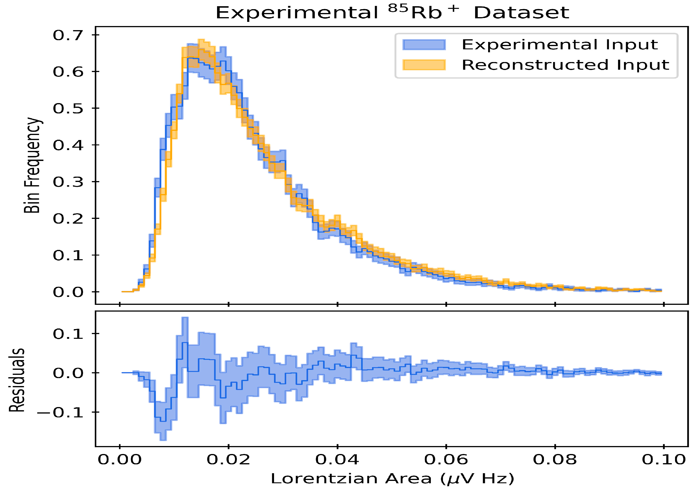
6.2. Predicted Ion Characteristics

After the classification of the experimental signals discussed above, the resulting filtered signal areas were binned over an appropriate range of values with sufficient granularity and normalized. At this point the data were in the proper format for the neural network and can be seen in Figure 8 as the experimental input histogram. After performing the network regression, the predicted parameters were identified and are summarized in Table 3.
Following the procedure outlined in Section 5.3, a comparison of the input and reconstructed output is shown in Figure 8.
From the results presented in Table 3, one can extrapolate the percent composition for a given number of ions from the Poisson mean. However, as established in the prior section, there is a known non-zero false-positive classification rate of ≈3.5% which is not accounted for by the DNN. Recall that the Poisson probability relationship is given by
Pr ( X = k ) =   μ p k e μ p k !
Pr ( X = 0 ) =   e μ p
where X is the discrete random variable (number of ions), and μ p is the Poisson mean. Using the fact that the ‘true’ percent of background signals is ( 1 + FPR ) e μ p , where FPR is the determined false-positive rate, the corrected Poisson mean can be shown to be
μ p , corr =   μ p ln ( 1 + FPR )
which is determined to be μ p , corr = 0.23 ( 6 ) for the measured FPR of 0.035 . Using this value, the expected percentages of 85Rb+ signals produced by different numbers of ions in SIPT are calculated: 79 ( 5 ) % correspond to background, 18 ( 4 ) % are single-ion measurements, and 2.3 ( 1.1 ) % are measurements of at least two ions.
Additionally, the ion position in the trap and SNR can be extrapolated from the predicted A single value using Equation (14), and were determined to be ρ / ρ 0 = 0.9 ( 3 ) and SNR = 0.21 ( 9 ) , respectively, at a 95% confidence level. These values lie within the allowed range of values and are reasonable.

7. Conclusions

In this paper, we first outlined two methods for the simulation of FT-ICR signals and provided a qualitative comparison between a rigorous, but intensive, approach to a simplified form. The two methods were shown to behave near-identically, and we discussed the advantages of the simpler method for the needs of this work. Then, we provided novel applications of supervised machine learning techniques for FT-ICR signal and background signal classification. This approach was motivated by the need for an efficient filtering of signals, the majority of which are expected to be background for experiments concerning nuclei delivered at the lowest rates. Next, we described a multi-layer densely connected deep neural network capable of accurately predicting collective ion characteristics in SIPT when provided with a large set of similar same-isotope signal information. While not used to perform the mass measurement itself, this neural network shows promise as an invaluable diagnostic tool during an experiment.
We have also provided validation and analysis for the classification network using both numerically simulated ion signals and experimental background data. The low false-positive ion signal classification rates of ≈10.5%, and ≈3.5% following filtering, are critical for experiments with the lowest ion delivery rates. Additionally, for future experimental campaigns of 100Sn+ the classifiers were shown to have accuracies of ≈65%, which are sufficient to successfully perform a mass measurement.
When evaluating the performance of the neural network, we qualitatively and visually compared the network input and reconstructed output for a unique sampling of numerically simulated datasets spanning a wide range of possible cases. Predictions of the most critical parameters μ p and A single in the simulated datasets showed agreement with the true value to 1 σ in all but one case. Ultimately, we demonstrated that the network provided robust predictions that accurately described the simulated ion characteristics. When applied to an experimental dataset, the neural network suggests that SIPT is sensitive to single-ion signals, predicting that 18(4)% of the experimental signals resulted from single ions.
This initial work in machine learning applications for precision mass measurements using the FT-ICR technique leaves open several avenues for future developments and improvements. Further investigation into feature set extraction for signal classification, such as including additional data beyond the Fourier spectrum, may improve the classifier’s ability to distinguish noise and ion signals. Implementing ensemble classification may also improve classification precision when considering diverse feature sets. Further refining of the neural network structure and training characteristics is needed for improved extraction of ion information. Additionally, lifting potentially limiting assumptions requires a significantly expanded training dataset and further explorations for an optimal neural network structure.

Author Contributions

Conceptualization and supervising by G.B., R.R. and S.S.; experiment and data collection by A.H. and R.R.; data analysis by S.E.C., A.H., W.K. and R.R.; software and code development by S.E.C., A.H., W.K. and R.R.; validation and analysis of results by S.E.C., A.H., W.K. and R.R.; initial draft writing of the manuscript by S.E.C.; editing, revising, finalizing of the manuscript by S.E.C., G.B., A.H., W.K., R.R. and S.S. All authors have read and agreed to the published version of the manuscript.

Funding

This work was conducted with the support of Michigan State University and the National Science Foundation, under Grant Nos. PHY-1102511, PHY-1126282, and PHY-2111185.

Data Availability Statement

The numerical and experimental data can be made available upon reasonable request.

Acknowledgments

Computational resources and services were provided by the Institute for Cyber-Enabled Research at Michigan State University.

Conflicts of Interest

The authors declare no conflict of interest. The funders had no role in the design of the study; in the collection, analyses, or interpretation of data; in the writing of the manuscript; or in the decision to publish the results.

References

  1. Brown, B.A.; Richter, W.A. New “USD” Hamiltonians for the sd shell. Phys. Rev. C 2006, 74, 034315. [Google Scholar] [CrossRef]
  2. Schatz, H.; Ong, W. Dependence of X-ray Burst Models on Nuclear Masses. Astrophys. J. 2016, 844, 139. [Google Scholar] [CrossRef]
  3. Lunney, D.; Pearson, J.M.; Thibault, C. Recent trends in the determination of nuclear masses. Rev. Mod. Phys. 2003, 75, 1021–1082. [Google Scholar] [CrossRef]
  4. Burbidge, E.M.; Burbidge, G.R.; Fowler, W.A.; Hoyle, F. Synthesis of the Elements in Stars. Rev. Mod. Phys. 1957, 29, 547–650. [Google Scholar] [CrossRef]
  5. Mumpower, M.; Surman, R.; McLaughlin, G.; Aprahamian, A. The impact of individual nuclear properties on r-process nucleosynthesis. Prog. Part. Nucl. Phys. 2016, 86, 86–126. [Google Scholar] [CrossRef]
  6. Baumann, T.; Hausmann, M.; Sherrill, B.; Tarasov, O. Opportunities for isotope discoveries at FRIB. Nucl. Instruments Methods Phys. Res. Sect. B Beam Interact. Mater. Atoms 2016, 376, 33–34. [Google Scholar] [CrossRef]
  7. Blaum, K. High-accuracy mass spectrometry with stored ions. Phys. Rep. 2006, 425, 1–78. [Google Scholar] [CrossRef]
  8. Brown, L.; Gabrielse, G. Geonium Theory: Physics of a single electron or ion in a penning trap. Rev. Mod. Phys. 1986, 58, 233. [Google Scholar] [CrossRef]
  9. Bollen, G.; Moore, R.; Savard, G.; Stolenzberg, H. The accuracy of heavy-ion mass measurements using time of flight-ion cyclotron resonance in a Penning trap. J. Appl. Phys. 1990, 68, 4355. [Google Scholar] [CrossRef]
  10. Eliseev, S.; Blaum, K.; Block, M.; Dörr, A.; Droese, C.; Eronen, T.; Goncharov, M.; Höcker, M.; Ketter, J.; Ramirez, E.M.; et al. A phase-imaging technique for cyclotron-frequency measurements. Appl. Phys. B 2014, 114, 107–128. [Google Scholar] [CrossRef]
  11. Haxel, O.; Jensen, J.H.D.; Suess, H.E. On the “Magic Numbers” in Nuclear Structure. Phys. Rev. 1949, 75, 1766. [Google Scholar] [CrossRef]
  12. Mayer, M.G. On Closed Shells in Nuclei. Phys. Rev. 1948, 74, 235–239. [Google Scholar] [CrossRef]
  13. Marshall, A.; Hendrickson, C.; Jackson, G. Fourier transform ion cyclotron resonance mass spectrometry: A primer. Mass Spectrom. Rev. 1998, 17, 1–35. [Google Scholar] [CrossRef]
  14. Kotsiantis, S.B.; Zaharakis, I.D.; Pintelas, P.E. Machine learning: A review of classification and combining techniques. Artif. Intell. Rev. 2006, 26, 159–190. [Google Scholar] [CrossRef]
  15. Schmidhuber, J. Deep learning in neural networks: An overview. Neural Netw. 2015, 61, 85–117. [Google Scholar] [CrossRef]
  16. Niu, Z.; Liang, H. Nuclear mass predictions based on Bayesian neural network approach with pairing and shell effects. Phys. Lett. B 2018, 778, 48–53. [Google Scholar] [CrossRef]
  17. Lovell, A.E.; Mohan, A.T.; Sprouse, T.M.; Mumpower, M.R. Nuclear masses learned from a probabilistic neural network. Phys. Rev. C 2022, 106, 014305. [Google Scholar] [CrossRef]
  18. Dong, X.X.; An, R.; Lu, J.X.; Geng, L.S. Novel Bayesian neural network based approach for nuclear charge radii. Phys. Rev. C 2022, 105, 014308. [Google Scholar] [CrossRef]
  19. Jiang, W.G.; Hagen, G.; Papenbrock, T. Extrapolation of nuclear structure observables with artificial neural networks. Phys. Rev. C 2019, 100, 054326. [Google Scholar] [CrossRef]
  20. Du, Y. Signal Enhancement and Data Mining for Chemical and Biological Samples Using Mass Spectrometry. Ph.D. Thesis, Purdue University, Ann Arbor, MI, USA, 2015. [Google Scholar]
  21. Nampei, M.; Horikawa, M.; Ishizu, K.; Yamazaki, F.; Yamada, H.; Kahyo, T.; Setou, M. Unsupervised machine learning using an imaging mass spectrometry dataset automatically reassembles grey and white matter. Sci. Rep. 2019, 9, 13213. [Google Scholar] [CrossRef]
  22. Williams, D.K.; Kovach, A.L.; Muddiman, D.C.; Hanck, K.W. Utilizing Artificial Neural Networks in MATLAB to Achieve Parts-Per-Billion Mass Measurement Accuracy with a Fourier Transform Ion Cyclotron Resonance Mass Spectrometer. J. Am. Soc. Mass Spectrom. 2009, 20, 1303–1310. [Google Scholar] [CrossRef] [PubMed]
  23. Williams, D.K., Jr. Exploring Fundamental Aspects of Proteomic Measurements: Increasing Mass Measurement Accuracy, Streamlining Absolute Quantification, and Increasing Electrospray Response. Ph.D. Thesis, North Carolina State University, Ann Arbor, MI, USA, 2009. [Google Scholar]
  24. Boiko, D.A.; Kozlov, K.S.; Burykina, J.V.; Ilyushenkova, V.V.; Ananikov, V.P. Fully Automated Unconstrained Analysis of High-Resolution Mass Spectrometry Data with Machine Learning. J. Am. Chem. Soc. 2022, 144, 14590–14606. [Google Scholar] [CrossRef] [PubMed]
  25. Nesterenko, D.A.; Eronen, T.; Ge, Z.; Kankainen, A.; Vilen, M. Study of radial motion phase advance during motion excitations in a Penning trap and accuracy of JYFLTRAP mass spectrometer. Eur. Phys. J. A 2021, 57, 302. [Google Scholar] [CrossRef]
  26. Jeffries, J.; Barlow, S.; Dunn, G. Theory of space-charge shift of ion cyclotron resonance frequencies. Int. J. Mass Spectrom. Ion Process. 1983, 54, 169–187. [Google Scholar] [CrossRef]
  27. Duhamel, P.; Vetterli, M. Fast fourier transforms: A tutorial review and a state of the art. Signal Process. 1990, 19, 259–299. [Google Scholar] [CrossRef]
  28. Payne, T.G.; Southam, A.D.; Arvanitis, T.N.; Viant, M.R. A signal filtering method for improved quantification and noise discrimination in fourier transform ion cyclotron resonance mass spectrometry-based metabolomics data. J. Am. Soc. Mass Spectrom. 2009, 20, 1087–1095. [Google Scholar] [CrossRef]
  29. Chiron, L.; van Agthoven, M.A.; Kieffer, B.; Rolando, C.; Delsuc, M.A. Efficient denoising algorithms for large experimental datasets and their applications in Fourier transform ion cyclotron resonance mass spectrometry. Proc. Natl. Acad. Sci. USA 2014, 111, 1385–1390. [Google Scholar] [CrossRef]
  30. Kanawati, B.; Bader, T.; Wanczek, K.P.; Li, Y.; Schmitt-Kopplin, P. FT-Artifacts and Power-function Resolution Filter in Fourier Transform Mass Spectrometry. Rapid Commun. Mass Spectrom. 2017, 31, 1607–1615. [Google Scholar] [CrossRef]
  31. Mathur, R.; O’Connor, P.B. Artifacts in Fourier transform mass spectrometry. Rapid Commun. Mass Spectrom. RCM 2009, 23, 523–529. [Google Scholar] [CrossRef]
  32. Comisarow, M.B.; Marshall, A.G. Frequency-sweep fourier transform ion cyclotron resonance spectroscopy. Chem. Phys. Lett. 1974, 26, 489–490. [Google Scholar] [CrossRef]
  33. Kilgour, D.P.A.; Wills, R.; Qi, Y.; O’Connor, P.B. Autophaser: An Algorithm for Automated Generation of Absorption Mode Spectra for FT-ICR MS. Anal. Chem. 2013, 85, 3903–3911. [Google Scholar] [CrossRef] [PubMed]
  34. Brustkern, A.M.; Rempel, D.L.; Gross, M.L. An electrically compensated trap designed to eighth order for FT-ICR mass spectrometry. J. Am. Soc. Mass Spectrom. 2008, 19, 1281–1285. [Google Scholar] [CrossRef] [PubMed]
  35. Lincoln, D.; Baker, R.; Benjamin, A.; Bollen, G.; Redshaw, M.; Ringle, R.; Schwarz, S.; Sonea, A.; Valverde, A. Development of a high-precision Penning trap magnetometer for the LEBIT facility. Int. J. Mass Spectrom. 2015, 379, 1–8. [Google Scholar] [CrossRef]
  36. Hamaker, A. Mass Measurement of the Lightweight Self-Conjugate Nucleus Zirconium-80 and the Development of the Single Ion Penning Trap. Ph.D. Thesis, Michigan State University, East Lansing, MI, USA, 2021. [Google Scholar]
  37. Johnson, J.B. Thermal Agitation of Electricity in Conductors. Phys. Rev. 1928, 32, 97–109. [Google Scholar] [CrossRef]
  38. Barry, J.R.; Lee, E.A.; Messerschmitt, D.G. Digital Communication; Springer: New York, NY, USA, 2004. [Google Scholar]
  39. Marshall, A.G. Theoretical signal-to-noise ratio and mass resolution in Fourier transform ion cyclotron resonance mass spectrometry. Anal. Chem. 1979, 51, 1710–1714. [Google Scholar] [CrossRef]
  40. Dahl, D.A. Simion for the personal computer in reflection. Int. J. Mass Spectrom. 2000, 200, 3–25. [Google Scholar] [CrossRef]
  41. Hossin, M.; Sulaiman, M.N. A review on evaluation metrics for data classification evaluations. Int. J. Data Min. Knowl. Manag. Process. 2015, 5, 1. [Google Scholar]
  42. Refaeilzadeh, P.; Tang, L.; Liu, H. Cross-Validation. In Encyclopedia of Database Systems; Liu, L., Özsu, M.T., Eds.; Springer: Boston, MA, USA, 2009; pp. 532–538. [Google Scholar] [CrossRef]
  43. Pedregosa, F.; Varoquaux, G.; Gramfort, A.; Michel, V.; Thirion, B.; Grisel, O.; Blondel, M.; Prettenhofer, P.; Weiss, R.; Dubourg, V.; et al. Scikit-learn: Machine Learning in Python. J. Mach. Learn. Res. 2011, 12, 2825–2830. [Google Scholar]
  44. Guyon, I.; Gunn, S.; Nikravesh, M.; Zadeh, L.A. Feature Extraction: Foundations and Applications; Springer: Berlin/Heidelberg, Germany, 2008; Volume 207. [Google Scholar]
  45. Pechenizkiy, M. The impact of feature extraction on the performance of a classifier: kNN, Naïve Bayes and C4.5. In Proceedings of the Conference of the Canadian Society for Computational Studies of Intelligence, Victoria, BC, Canada, 9–11 May 2005; Springer: Berlin/Heidelberg, Germany, 2005; pp. 268–279. [Google Scholar]
  46. Smith, J.O. Mathematics of the Discrete Fourier Transform (DFT): With Audio Applications; W3K Publishing, 2008. [Google Scholar]
  47. Diamantidis, N.; Karlis, D.; Giakoumakis, E. Unsupervised stratification of cross-validation for accuracy estimation. Artif. Intell. 2000, 116, 1–16. [Google Scholar] [CrossRef]
  48. Snoek, J.; Larochelle, H.; Adams, R.P. Practical Bayesian Optimization of Machine Learning Algorithms. In Proceedings of the Advances in Neural Information Processing Systems, Tahoe, NV, USA, 3–6 December 2012; Pereira, F., Burges, C., Bottou, L., Weinberger, K., Eds.; Curran Associates, Inc.: Red Hook, NY, USA, 2012; Volume 25. [Google Scholar]
  49. Head, T.; MechCoder; Louppe, G.; Shcherbatyi, I.; Fcharras, Z.V.; cmmalone; Schröder, C.; nel215; Campos, N. scikit-optimize v0.5.2, 2018. [CrossRef]
  50. Svozil, D.; Kvasnicka, V.; Pospichal, J. Introduction to multi-layer feed-forward neural networks. Chemom. Intell. Lab. Syst. 1997, 39, 43–62. [Google Scholar] [CrossRef]
  51. Chollet, F. Keras. 2015. Available online: https://keras.io (accessed on 18 May 2022).
  52. Agarap, A.F. Deep Learning using Rectified Linear Units (ReLU). arXiv 2018, arXiv:1803.08375. [Google Scholar]
  53. Srivastava, N.; Hinton, G.; Krizhevsky, A.; Sutskever, I.; Salakhutdinov, R. Dropout: A simple way to prevent neural networks from overfitting. J. Mach. Learn. Res. 2014, 15, 1929–1958. [Google Scholar]
  54. Kingma, D.; Ba, J. Adam: A Method for Stochastic Optimization. Int. Conf. Learn. Represent. 2014, arXiv:1412.6980. [Google Scholar] [CrossRef]
  55. Gurney, K. An Introduction to Neural Networks; CRC Press: Boca Raton, FL, USA, 2018. [Google Scholar]
  56. Gal, Y.; Ghahramani, Z. Dropout as a Bayesian Approximation: Representing Model Uncertainty in Deep Learning. In Proceedings of the 33rd International Conference on Machine Learning, New York, NY, USA, 20–22 June 2016; Balcan, M.F., Weinberger, K.Q., Eds.; PMLR: New York, NY, USA, 2016; Volume 48, pp. 1050–1059. [Google Scholar]
  57. Yeung, D.S.; Cloete, I.; Shi, D.; wY Ng, W. Sensitivity Analysis for Neural Networks; Springer: Berlin/Heidelberg, Germany, 2010. [Google Scholar]
Figure 1. Frequency spectra for Fourier transform ion cyclotron resonance signals from the single-ion Penning trap (SIPT) for various measured and simulated 85Rb+ ion signals. The black line indicates the experimental dataset, the dashed red line shows one possible Lorentzian distribution fit to the dataset. Top Left: Example of a measured SIPT signal, likely from real ions, easily distinguished from noise as a strong peak is present near the expected frequency. Top Right: A measured signal which is ambiguous as the identified peak frequency may also just be noise. Bottom Left: Example of a simulated noise signal which exhibits a strong peak near the expected frequency, easily mistaken for a signal produced by an ion. Bottom Right: A simulated signal created by two ions whose peak frequency is easily mistaken for noise due to destructive interference.
Atoms 11 00126 g001
Figure 2. A cartoon illustration of the single-ion Penning trap ring electrode configuration and detection scheme. The shown configuration is optimal for dipole pickup of the ν + eigenfrequency. The red electrodes labeled ‘P’ are those used for signal pickup, and those labeled ‘0’ are grounded or used for radio frequency excitations.
Atoms 11 00126 g002
Figure 3. Power spectral density (PSD) for measured background data, compared to simulated white noise (of Equation (7)). The average of 1500 samples of each of the measured and simulated data are plotted above. The PSD is calculated over a 100 Hz bandwidth, centered about the reduced cyclotron frequency of 85Rb+. The mean values of the averaged measured signal and white noise amplitude were optimized to be as close as possible.
Atoms 11 00126 g003
Figure 4. A comparison of the signal-to-noise (SNR) ratio distributions for N = 1 , 2 , 3 ions in the SIPT. Three different phase spread distributions are investigated, with each plot comparing the ‘sum of sines’ approach (top) of Equation (11) to the rigorous method of [9] (middle), and the residuals between the two methods (bottom). For each ion number, 10 4 simulated signals make up each distribution.
Atoms 11 00126 g004
Figure 5. Impact of the included frequency range for the feature set on classification precision. Each feature set is a sampling from the discrete Fourier transform of the SIPT time-domain signals, which had a zero padding of twice the signal length on both the left and right sides. Note that typical SIPT signals are expected to have an FWHM of ≲10 Hz. Classifier precision was determined from a 10-fold cross-validation approach with a total of 10,000 samples. Four classifiers were considered: k-nearest neighbors (kNN), Gaussian naive Bayes (GNB), support vector machine (SVM), and logistic regression (LR).
Atoms 11 00126 g005
Figure 6. Precision of classifiers for different simulated single-ion signal-to-noise (SNR) ratios. Four classifiers were considered: k-nearest neighbors (kNN), Gaussian naive Bayes (GNB), support vector machine (SVM), and logistic regression (LR). SNR values ranging from ∼ 0.25 to ∼ 0.55 over a 100 Hz spectral bandwidth are investigated, as these are expected values for single-ion signals. Precision was determined by training each classifier in a 5-fold cross-validation approach with a dataset of size 20,000.
Atoms 11 00126 g006
Figure 7. Investigation of the neural network sensitivity for six unique simulated datasets. Sensitivity is determined by the residual between a given input ‘A’ and another input ‘B’ generated using the output parameters predicted by the initial input. Small residuals are desired. Note that the input to the neural network is a histogram of Lorentzian areas, defined by Equation (6), for a large set of SIPT FT-ICR frequency-domain signals. The reconstruction for input ‘B’ uses 80,000 ion signals to produce each histogram shown. A summary of the corresponding output parameters can be found in Table 2.
Atoms 11 00126 g007
Figure 8. Comparison of a histogram of experimental 85Rb+ SIPT signal Lorentzian areas (defined by Equation (6)) to a histogram of 80,000 simulated 85Rb+ SIPT signals which was generated from the parameters predicted by the neural network; summarized in Table 3. Small residuals correspond to both reasonable predictions from the neural network as well as reasonable simulations of the SIPT FT-ICR signals.
Atoms 11 00126 g008
Table 1. Summary of the optimal model hyperparameters found using a Bayesian optimization for four classifiers: k-nearest neighbors (kNN), Gaussian naive Bayes (GNB), support vector machine (SVM), and logistic regression (LR). Classifier precision was determined from a cross-validation approach with 10,000 samples. The signals with ions present were chosen to have SNR = 0.23 normally distributed with an uncertainty of σ SNR = 0.05 .
ClassifierParameterValuePrecision
kNNAlgorithmBall Tree0.711
Leaf Size46
k Neighbors35
GNBVariable Smoothing00.704
SVMC1000.715
γ 1.895
Degree8
Kernelrbf
LRC390.735
SolverSaga
Penalty2
Table 2. A summary of the true and predicted parameters from the neural network for six unique simulated datasets. All predicted values are determined to 1 σ uncertainty, calculated using the MC Dropout method [56] for 100 iterations. Summaries for each output parameter can be found in Section 5.2.
Sim. Dataset 0Sim. Dataset 1Sim. Dataset 2
TruePredictionTruePredictionTruePrediction
μp0.540.54(8)0.370.43(8)0.140.18(6)
Asingle (mV)0.0530.053(5)0.0510.051(3)0.0460.044(2)
σ(Asingle) (mV)0.0008350.0017(9)0.001740.0023(8)0.0003570.0024(7)
Voffset (μV)8.898.1(1.1)9.798.4(1.0)1.850.9(8)
ϕ 0 , max (rad)4.854(1)1.911.8(1.0)4.473.8(9)
Sim. Dataset 3Sim. Dataset 4Sim. Dataset 5
TruePredictionTruePredictionTruePrediction
μp0.360.37(7)0.120.18(7)0.290.34(8)
Asingle (mV)0.0270.029(3)0.0540.049(3)0.0520.053(5)
σ(Asingle) (mV)0.0004040.000264(12)0.0003770.003(6)0.0000780.00015(10)
Voffset (μV)8.667.7(9)4.454.0(5)9.738.8(1.1)
ϕ 0 , max (rad)3.84.1(7)3.443.2(9)5.534.2(1.1)
Table 3. Neural network predictions on the experimental 85Rb+ dataset. Summaries for each output parameter can be found in Section 5.2.
Prediction
μ p 0.26(6)
A single (mV)0.022(4)
σ ( A single ) (mV)0.0024(5)
Voffset (μV)2.0(7)
ϕ 0 , max (rad)4.3(1.4)
Disclaimer/Publisher’s Note: The statements, opinions and data contained in all publications are solely those of the individual author(s) and contributor(s) and not of MDPI and/or the editor(s). MDPI and/or the editor(s) disclaim responsibility for any injury to people or property resulting from any ideas, methods, instructions or products referred to in the content.

