Article

Relativistic Atomic Structure of Au IV and the Os Isoelectronic Sequence: Opacity Data for Kilonova Ejecta

1
Department of Physics and Astronomy, Center for Simulational Physics, The University of Georgia, Athens, GA 30602, USA
2
Department of Physics, Auburn University, Auburn, AL 36849, USA
3
104 Kinard Laboratory, Department of Physics and Astronomy, Clemson University, Clemson, SC 29634, USA
*
Author to whom correspondence should be addressed.
Atoms 2022, 10(3), 94; https://doi.org/10.3390/atoms10030094
Submission received: 14 July 2022 / Revised: 26 August 2022 / Accepted: 4 September 2022 / Published: 13 September 2022

Abstract

:
Direct detection of gravitational waves (GWs) on 17 August 2017, propagating from a binary neutron star merger, or a “kilonova”, opened the era of multimessenger astronomy. The ejected material from neutron star mergers, or “kilonova”, is a good candidate for optical and near infrared follow-up observations after the detection of GWs. The kilonova from the ejecta of GW1780817 provided the first evidence for the astrophysical site of the synthesis of heavy nuclei through the rapid neutron capture process or r-process. Since properties of the emission are largely affected by opacities of the ejected material, enhancements in the available r-process data is important for neutron star merger modeling. However, given the complexity of the electronic structure of these heavy elements, considerable efforts are still needed to converge to a reliable set of atomic structure data. The aim of this work is to alleviate this situation for low charge state elements in the Os-like isoelectronic sequence. In this regard, the general-purpose relativistic atomic structure packages (GRASP 0 and GRASP2K) were used to obtain energy levels and transition probabilities (E1 and M1). We provide line lists and expansion opacities for a range of r-process elements. We focus here on the Os isoelectronic sequence (Os I, Ir II, Pt III, Au IV, Hg V). The results are benchmarked against existing experimental data and prior calculations, and predictions of emission spectra relevant to kilonovae are provided. Fine-structure (M1) lines in the infrared potentially observable by the James Webb Space Telescope are highlighted.

1. Introduction

The usefulness of gravitational wave observations is now well established, where focus has been on the detection of merging black holes [1]. However, one of the most promising applications of gravitational wave studies was revealed with the first detection of merging neutron stars and their role in producing heavy elements [2]. It has been established that low-mass elements C, N, O, …, Mg, and up to Mo, are produced in low-mass stars, while iron-peak elements are produced in the explosive ejecta of supernovae. Numerous observations and robust nucleosynthesis models confirm this scenario [3,4]. For heavier elements that require a rapid neutron capture (r-process) mechanism, the details of their production mechanism are an area of active study.
It was postulated as early as 1957 by Cameron that the merger of binary neutron stars would result in a neutron-rich ejecta that could produce these heavy elements. One of the early nucleosynthesis models which predicted the yields of such events was given by Freiburghaus et al. [5]. The detection of a neutron star merger (NSM) [6] event and the spectral observation of its optical and infrared emission opens up the possibility of direct interrogation of the formation site of these heavy r-process elements. However, interpretation, analysis, and modeling of the observed optical/IR spectra is hindered by the sparsity of atomic opacity studies for these r-process elements, particularly beyond Mo.
Recent work on atomic data for neutron star merger modeling has focused on providing complete coverage for a wide range of heavy elements [7,8,9]. In this paper we focus on a small number of ion stages, with the aim of providing calculations that have been tailored for each charge state. We also note that the inclusion for non-dipole radiative rates in the calculation also allows for a line list that includes lines that could be observed by the James Webb Space Telescope.
Our goal is to provide additional large-scale, but reliable, atomic line lists for Re-Pt ( Z = 75 79 ). Thus atomic data, such as wavelengths, spectroscopic labels, and transition probabilities are needed. While there are many computational methods based on perturbation or variational theory that could be adopted, we focus on general multiconfiguration variational methods where the wave function for an atomic state is determined in terms of a basis of configuration state functions (CSFs). In particular, the multiconfiguration Dirac–Hartree–Fock (MCDHF) method with Breit and quantum electrodynamics (QED) corrections [10] as implemented in the General purpose Relativistic Atomic Structure Package (GRASP) [11,12] is adopted. This fully relativistic code constructs and diagonalizes a Dirac–Coulomb Hamiltonian to produce relativistic orbitals, which are then used in a multiconfiguration Dirac–Fock calculation. Despite GRASP0 and GRASP2K calculations often having smaller configuration sets than those possible with other codes, we note that the underlying method is considered to be of high accuracy, allowing for accurate energies for complex species such as those considered here. In addition, a large number of lines are produced from the calculations presented, with more than 69,000 E1 and M1 transitions for each ion considered here.
The atomic data that are needed for spectral and neutron star merger modeling includes wavelengths of emission lines (hence energies from the atomic structure), and E1 and M1 spontaneous emission rates. It is also useful to produce derived coefficients that can be directly used by modelers. One particularly useful coefficient is known as an expansion opacity. In an expanding object, the frequency of the photons suffers a continuous Doppler shift with respect to the rest frame of the material. Thus each photon has an increased probability of interacting with a line; this enhanced effect of spectral lines can be taken into account as an expansion opacity [13].
In this manuscript we focus on the Os isoelectronic sequence (Os I, …, Hg V), because it covers elements likely to be made in neutron star mergers and is confined to the lower charge states likely to be present. We note that work on other isoelectronic sequences is also underway. Section 2 describes the relativistic atomic structure theory adopted here, relations for emission spectra, and opacities in the local thermodynamic equilibrium (LTE) approximation. Section 3 gives a discussion of our results, while a summary and outlook for future work is given in Section 4.

2. Atomic Structure Calculations: GRASP 0 and GRASP2K

2.1. Grasp

The GRASP 0 package is based on the Oxford multiconfiguration Dirac–Fock (MCDF) [14] and higher-order corrections (MCBP/BENA) [15] codes published in 1980. The package is used to compute atomic energy levels, orbitals, and transition data within the relativistic formalism.
The GRASP2K package [12] is a later iteration of GRASP 0 and based on the fully relativistic multiconfiguration Dirac–Hartree–Fock (MCDHF) method [16]. The package consists of a number of application programs and tools to compute approximate relativistic wave functions, energy levels, hyperfine structures (HFS), isotope shifts (IS), Lande g-factors, interactions with external fields, angular couplings for labeling purposes, transition energies, and transition probabilities for many-electron atomic systems. We use both of these codes as a means of checking the convergence of the calculations and to give an indication of the approximate uncertainties in the final results.

2.2. Multiconfiguration Dirac–Hartree–Fock (MCDHF)

In the relativistic multiconfiguration Dirac–Hartree–Fock (MCDHF) method, the Dirac–Coulomb Hamiltonian is given by,
H D C = i = 1 N [ c α i · p i + ( β i 1 ) c 2 + V n u c ( r i ) ] + i > j N 1 r i j ,
where V n u c is the electron-nucleus coulomb interaction, r i j is the distance between electrons i and j, and α and β are the Dirac matrices. The wave function is represented by an atomic state function (ASF), ψ ( γ P J ) , expanded in a set of configuration state functions (CSFs), Φ ( γ P J ) ,
ψ ( γ P J ) = j = 1 N C S F c j Φ ( γ j P J ) .
Here γ specifies CSF properties including orbital occupancy and subshell quantum numbers in the angular momentum coupling tree, P is parity, J is the final angular quantum number, and c j are the expansion coefficients. The CSFs can be expressed as products of one-electron solutions of the Dirac equation which can be written as,
ψ n l s j m ( r , θ , ϕ ) = 1 r P n l j ( r ) Ω l s j m ( θ , ϕ ) i Q n l j ( r ) Ω l ˜ s j m ( θ , ϕ ) ,
where P n l j ( r ) and Q n l j ( r ) are called the regular and irregular solutions, and Ω l s j m ( θ ϕ ) are built from the coupling of the spherical harmonics Y l m l ( θ , ϕ ) and the spin functions χ m s ( 1 / 2 ) . n, l, j, and s, are the usual principal, orbital angular momentum, total angular momentum, and spin angular momentum quantum numbers, respectively, while m l is the projection of l and m s the projection of s on the z quantization axis. l and l ˜ are related to each other [17],
l ˜ = l + 1 , j = l + 1 / 2 l 1 , j = l 1 / 2 .
If the quantum number κ is introduced as the eigenvalue of the operator K = 1 l σ , where σ is the Pauli matrix,
κ = ( l + 1 ) , j = l + 1 / 2 ( κ n e g a t i v e ) + l , j = l 1 / 2 ( κ p o s i t i v e ) ,
then we can rewrite Equation (3) as,
ψ n κ m ( r , θ , ϕ ) = 1 r P n κ ( r ) Ω κ m ( θ , ϕ ) i Q n κ ( r ) Ω κ m ( θ , ϕ ) .
The lists of CSFs that defines the ASF, mixing coefficients, and orbital parts of the wave functions are the basis for the GRASP2K program. Thus, the choice of CSFs affects the accuracy of the calculated energies and transition probabilities. In the work to be presented here we perform GRASP 0 and GRASP2K computations with a range of CSFs, as described in Section 3.

2.3. LTE Spectra and Expansion Opacity

The environment in the kilonova ejecta at early times is expected to be of a sufficiently high density that the populations of the electronically excited states are considered to be thermalized, i.e., the ejecta gas density exceeds the critical density of the individual levels. The critical density is the gas density required to drive the populations of the individual levels to their thermodynamic values. Therefore, we can consider the emission or absorption to be in local thermodynamic equilibrium (LTE). In this regard, the line intensities are obtained from,
I ( i , k ) = F ( i ) A k i ,
where A k i is the transition probability and F ( i ) is the relative LTE population for level i. The absorption oscillator strength f i k is given by
f i k = λ 2 6.6702 × 10 15 g k g i A k i ,
where g i and g k are the statistical weights for the lower and upper level of a spectral line which are obtained from the appropriate angular momentum quantum numbers, g i ( k ) = 2 J i ( k ) + 1 . F ( i ) is given by
F ( i ) = ( 2 J i + 1 ) exp ( Δ E / k T ) / Q ,
with Δ E = E i E 1 and the internal partition function, Q,
Q = i = 1 ( 2 J i + 1 ) exp ( Δ E / k T ) ,
assuming a Boltzmann distribution of level populations [18].
Following Kasen et al. [19], the expansion opacity for bound-bound transitions is given by
κ ex ( λ ) = 1 c t ej ρ i , k λ i k Δ λ [ 1 exp ( τ i k ) ] ,
where the optical depth τ i k is
τ i k = π e 2 m e c f i k n i t ej λ i k ,
where n i is the number density in the lower state of the ion in question, t ej is the time since the merger, and ρ is the ejecta density. From Kasen et al. [19], we adopt the typical values ρ = 10 13 g cm 3 , t ej = 1 day, and the wavelength binning Δ λ = 0.01 λ . Note that these expansion opacities are provided for illustrative purposes showing the use of the fundamental data and to allow us to explore the effects of the atomic data on opacities. We assume the gas to be completely composed of only one ion. The data user can also generate their own opacities from the fundamental data including relevant mixtures of ions.

3. Results and Discussions

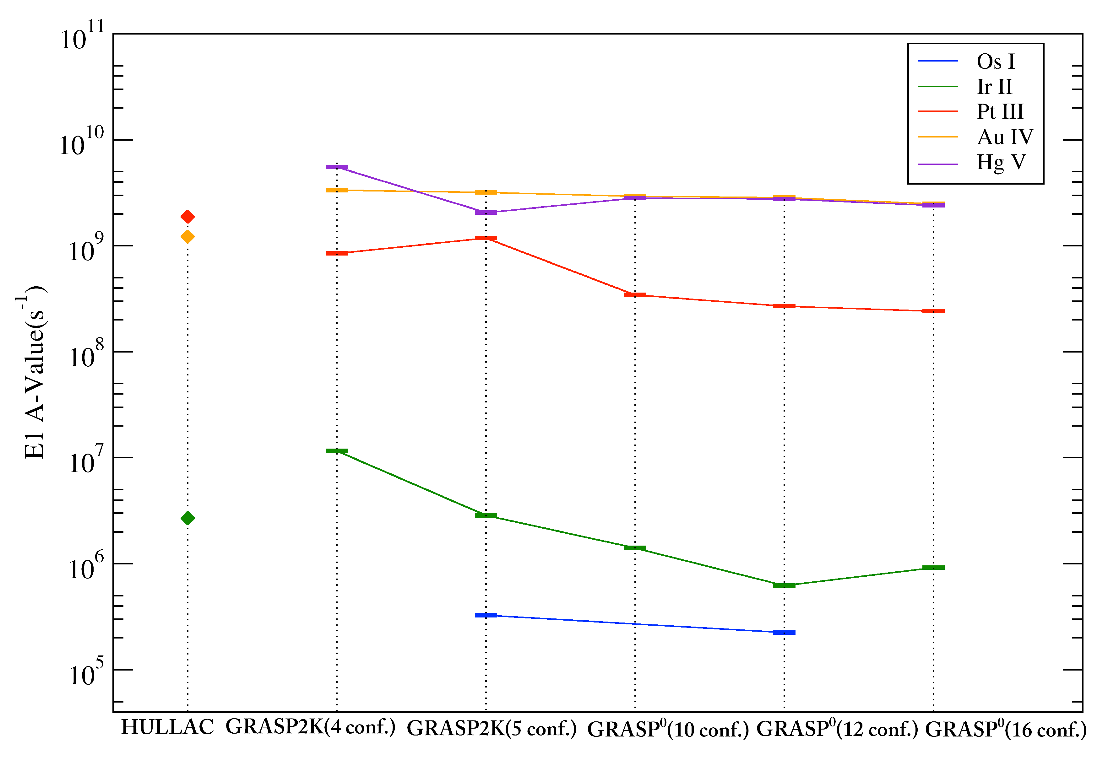
3.1. Energy Levels and Transition Probabilities

We have calculated energy levels and transition probabilities for the Os isoelectronic sequence using the GRASP 0 and GRASP2K codes. The NIST Atomic Spectral Database [20] has energies for some of the Os I [21] and Ir II [22] levels. Moreover, some calculations have been evaluated by Gillanders et al. [23], and Ryabtsev et al. [24] for Pt III, and the HULLAC code has been used to compute atomic data for Os I, Ir II, Pt III, and Au IV [8,25], for E1 transitions.
Our choice of adopted electron configurations is given in Table 1, which includes the ground configuration and the configurations likely to dominate the expansion opacity under the low temperature radiation field conditions of the kilonova. This means that we focused on low-lying configurations. Thus, in the GRASP2K calculation we included 5 d 6 6 s 2 , 5 d 6 6 s 6 p , 5 d 7 6 s , 5 d 7 6 p , and 5 d 8 . In the GRASP 0 calculations, we performed three different computations with increasingly larger numbers of configurations to allow for convergence checks, with the configurations for the three calculations (10, 12, and 16 configurations) being shown in Table 1. However, it was found that convergence could be obtained in the GRASP2K calculations with smaller configuration sizes.
Figure 1 shows energy level diagrams for Figure 1a Os I, Figure 1b Ir II, Figure 1c Pt III, Figure 1d Au IV, and Figure 1e Hg V obtained from GRASP2K and GRASP 0 calculations using the target model in Table 1 as the reference configurations. Comparison is made to theoretical data calculated using the HULLAC code [8,25] and experimental data from the NIST database when available [20]. Moreover, in GRASP2K we used four and five reference configurations; for four configurations the 5 d 6 6 s 2 was omitted. Since the ground level is 5 d 6 6 s 2 for Os I, the 5 d 8 was omitted in that case. In general, the GRASP2K energies are in better agreement with the NIST values than the GRASP 0 energies for the lower lying configurations. The GRASP 0 calculations show some improvement in the energies for certain levels, while in most cases the comparison is mixed. As a consequence, we adopt the GRASP2K results for the expansion opacities later in this paper.
The energy levels of Os I and Ir II are given in Table 2 and Table 3, respectively, and are compared with energies from GRASP 0 , NIST [20], HULLAC calculations [8,25], DESIRE [26], and experimental studies of Ir II [27]. Although levels in the ground term are in good agreement with the NIST and DESIRE data, there are deviations from the NIST database for both GRASP2K and GRASP 0 results for the higher energy levels. For Pt III, Au IV, and Hg V, literature on the energy level structures is sparse. For Pt III, a GRASP 0 calculation [23], and some experimental and theoretical results by Ryabtsev et al. [24] are available. For the remainder of the Os-sequence, we are limited to comparisons between the present GRASP 0 and GRASP2K calculations.
Table 4 gives as an example the convergence of energy eigenvalues for levels in the ground term of each of the considered ions from the current calculations. Here we give energies for all GRASP 0 and GRASP2K results. In all cases, the ground level is correctly predicted and the ordering of J-levels is consistent.
Computed energies for low-lying levels of Pt III are compared in Table 5 from our GRASP2K(5) calculations to those of Gillanders et al. [23], Ryabtsev et al. [24], and the HULLAC calculations [8,25], while comparisons to the two M1 transition probabilities given in Gillanders et al. [23] are also shown. There is general agreement amongst the calculations except for the energy of the 5 D 4 state, and our M1 values are 36–52% smaller than those computed by Gillanders et al. [23].
Transition probabilities for E1 vs. wavelength are plotted in Figure 2 for Figure 2a Os I, Figure 2b Ir II, Figure 2c Pt III, Figure 2d Au IV, and Figure 2e Hg V. The strongest transitions occur at shorter wavelengths, with most of them being shorter than 200 nm. We note that, while the bulk of the transitions are at UV wavelengths, the density of lines may make this wavelength range difficult to use for line identification. Observing at longer wavelengths, where the lines are more sparse, may provide opportunities for more definitive identification of the charge state of the ion (see below). The weighted transition probabilities ( g A , where g = 2 J + 1 ), are compared with HULLAC calculations [8,25] and DESIRE [26] for Os I [28] and Ir II [27] in Table 6 and Table 7, respectively. There is reasonable agreement between GRASP2K and DESIRE, and GRASP2K and HULLAC calculations. The average percent difference of Os I is 113 % , and 126 % , and the average percent difference of Ir II is 63.5 % , and 82.7 % , between GRASP2K and DESIRE, and GRASP2K and HULLAC calculations, respectively. To illustrate the convergence of the A-values with calculation size, an electron dipole transition present in all ions was selected. The A-value for the various calculations is plotted in Figure 3, showing a reasonable convergence for all members of the iso-electronic sequence. The reason for choosing 5 d 8 3 F 5 d 7 ( 2 H 3 ) 6 p 3 G transition is that for most of the ions in this paper, this transition has the strongest A-value, as shown in Table 8. DESIRE does not provide this transition. Increasing the number of configurations was observed to have a minor impact on the transition rates of the most highly ionized systems in the Os-sequence. However, near-neutral systems (e.g., Ir II) show slower convergence with respect to increasing numbers of configurations.

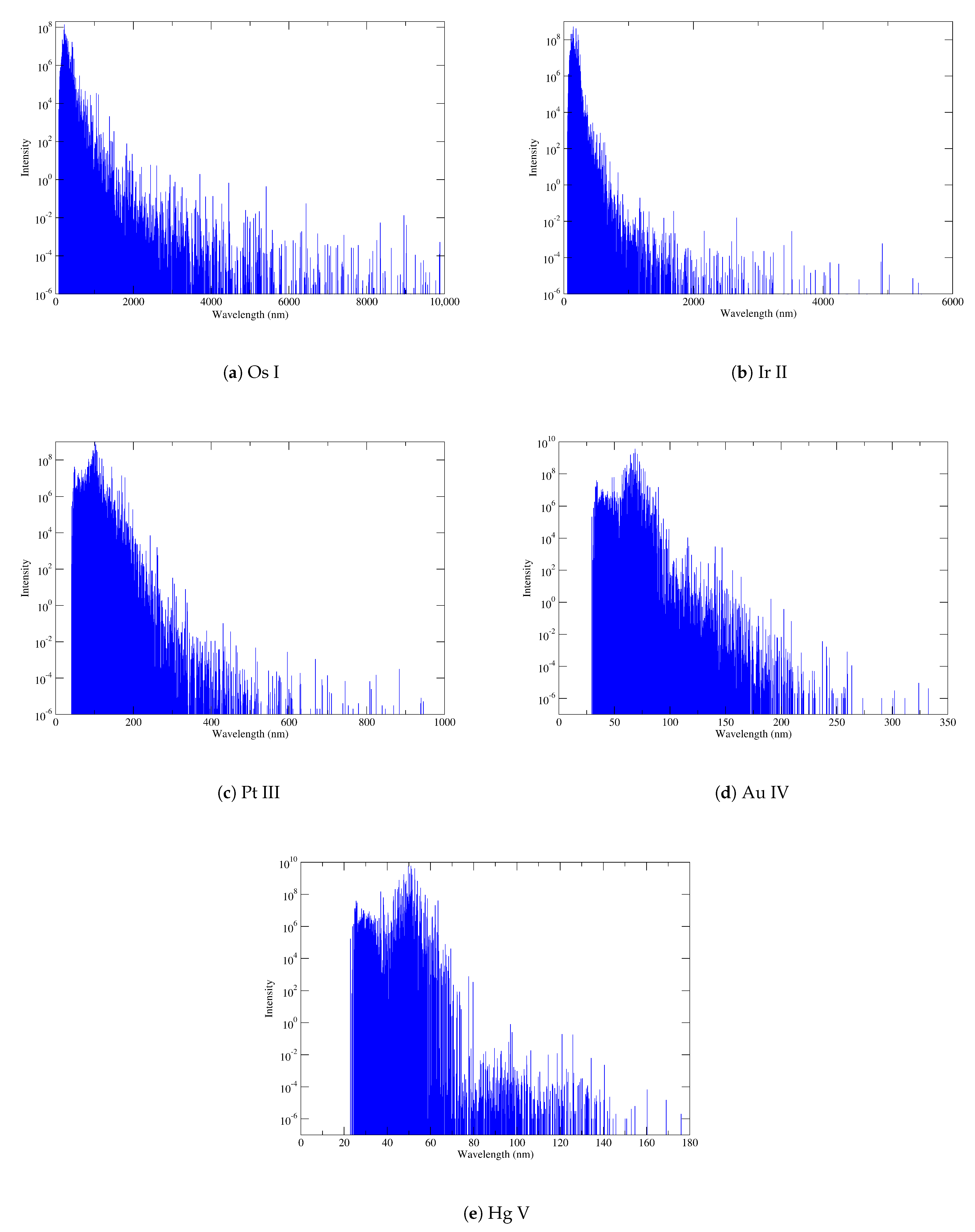
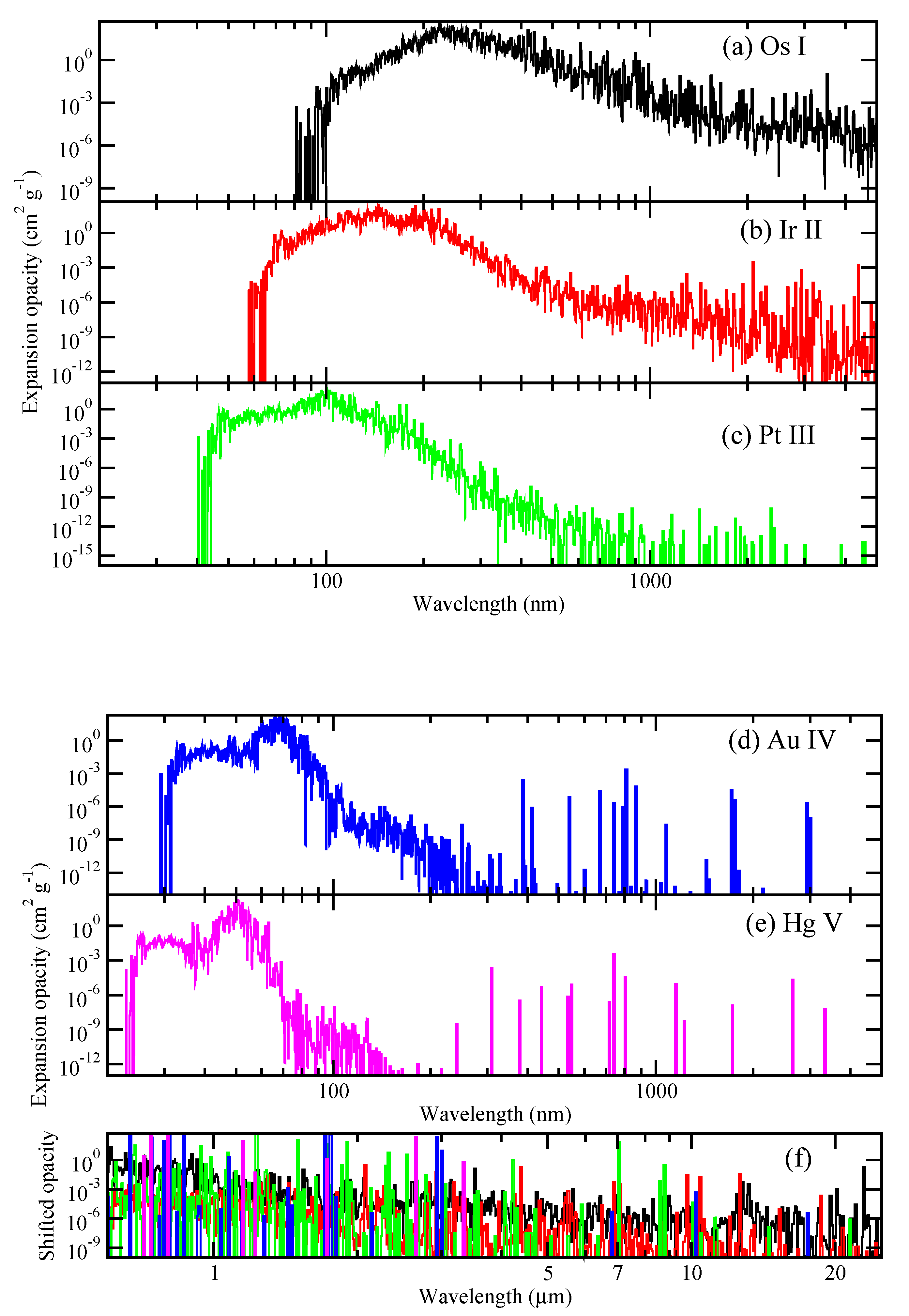
3.2. LTE Spectra and Expansion Opacities

The temperature in neutron star merger ejecta is approximately 5000 K, and cooling off to 1000 K at later times. Therefore, as an illustration, the LTE spectra for Os I, Ir II, Pt III, Au IV, and Hg V at 5000 K are computed and displayed for E1 transitions in Figure 4. The emission lines are very dense in the UV and visible, but become less crowded as the wavelength increases into the IR. Moreover, wavelengths of the three most intense lines for each ion are represented in Table 8.
In Figure 5, we plot the expansion opacity as given by Equation (11) for each of the ions considered in this work. To facilitate comparison to prior studies [8,19], the opacity is computed for t = 1 day and ρ = 10 13 g/cm 3 with wavelength binning of Δ λ = 0.01 λ . We choose a temperature of 3700 K as it is representative of a kilonova. The opacity peaks in the visible shifting into the UV with increasing ion charge from ∼225 nm for Os I to ∼50 nm for Hg V similar to the behavior of the LTE spectra in Figure 4. Further, as the ion charge increases, a number of IR lines appear with increasing strength over a less crowded background.
Figure 5f provides a comparison of the IR lines within the wavelength window of the James Webb Space Telescope (JWST) for 5–25 μ m. The background opacity magnitude in Figure 5f have been shifted to facilitate comparison of the lines for the various ions. A number of very prominent features emerge from the background and it is expected that in the mid-IR these features will be in emission. Table 9 lists the three most dominant transitions per ion which we predict may be observable by the Near Infrared Spectrograph (NIRSpec) or the Mid Infrared Instrument (MIRI) on JWST for a kilonova, particularly at late times. However, there is some uncertainty in the line positions as many transitions are between excited states for which there are very little experimental data; exceptions are for some lines due to Os I, Ir II, and Au IV as indicated in Table 9. The IR lines correspond primarily to M1 transitions within the ground configuration, and therefore the corresponding levels should be readily populated in the low temperature kilonova ejecta.
For Pt III, Gillanders et al. [23] predict the 3 F 3 3 F 4 line to occur at 1.092 μ m, while the current work predicts the wavelength to be 1.234 μ m. This aligns with a feature at 8.7 days in the observed spectrum of AT2017gfo. Further, a broad line centered near 1 μ m may be explained by a cluster of Pt III lines at 0.947, 0.949, 0.991, and 1.077 μ m (see Figure 5f and Figure 4 of Gillanders et al. [23]). However, MIRI/JWST observations near 7 μ m and 8.7 μ m may be the best hope of identifying platinum in a kilonova, as illustrated in the current Figure 5f.

4. Summary

In this work, we have performed atomic structure calculations for Os I (Z = 76), Ir II (Z = 77), Pt III (Z = 78), Au IV (Z = 79), and Hg V (Z = 80) to construct atomic data for r-process elements. By using two different atomic code packages, GRASP2K and GRASP 0 , energy levels, and transition probabilities (E1 and M1) for the above ions were computed.
A list of the strongest transitions are given for each ion in the UV for E1 transitions and in the IR for M1 transitions. It is pointed out that the possible identification of r-process elements will be easier in the near- to mid-IR in the nebula phase of a kilonova and the M1 lines are far less crowded in this spectral window. The calculated data are made available in standard formats for use in the modeling of neutron star mergers at www.physast.uga.edu/ugamop/ (accessed on 2 September 2022).
Given the complex environment of a neutron star merger ejecta, future work should consider electron impact excitation to enable non-LTE spectra effects and magnetic field effects on atomic structure.

Author Contributions

Formal analysis, Z.S.T., B.M., Y.W. and A.F.; investigation, Z.S.T. and B.M.; conceptualization and methodology, S.L., P.S. and S.B.; writing—original draft preparation, Z.S.T.; writing—review and editing, all authors; visualization, Z.S.T. and P.S.; project administration and funding acquisition, S.L., J.M., C.S. and P.S. All authors have read and agreed to the published version of the manuscript.

Funding

This work was partially supported by NSF grant 1816984.

Data Availability Statement

All data can be available in Cloudy/Stout format from the UGA Molecular Opacity Project website: https://www.physast.uga.edu/ugamop/index1.html (accessed on 2 September 2022).

Acknowledgments

B.M. McLaughlin acknowledges the University of Georgia at Athens for the award of an adjunct professorship and Queen’s University Belfast for a visiting research fellowship (vrf). This work was supported in part by resources and technical expertise from the UGA Georgia Advanced Computing Resource Center (gacrc). The authors also gratefully acknowledge the Gauss Centre for Supercomputing e.V. for funding this project by providing computing time on the GCS Supercomputer hazel hen at Höchstleistungsrechenzentrum Stuttgart.

Conflicts of Interest

The authors declare no conflict of interest.

References

  1. Abbott, B.P.; Abbott, R.; Abbott, T.; Abernathy, M.; Acernese, F.; Ackley, K.; Adams, C.; Adams, T.; Addesso, P.; Adhikari, R.; et al. Observation of gravitational waves from a binary black hole merger. Phys. Rev. Lett. 2016, 116, 061102. [Google Scholar] [CrossRef] [PubMed]
  2. Wanajo, S.; Sekiguchi, Y.; Nishimura, N.; Kiuchi, K.; Kyutoku, K.; Shibata, M. Production of all the r-process nuclides in the dynamical ejecta of neutron star mergers. Astrophys. J. Lett. 2014, 789, L39. [Google Scholar] [CrossRef]
  3. Nomoto, K.; Tominaga, N.; Umeda, H.; Kobayashi, C.; Maeda, K. Nucleosynthesis yields of core-collapse supernovae and hypernovae, and galactic chemical evolution. Nucl. Phys. A 2006, 777, 424–458. [Google Scholar] [CrossRef]
  4. Grimmett, J.; Heger, A.; Karakas, A.I.; Müller, B. Nucleosynthesis in primordial hypernovae. Mon. Not. R. Astron. Soc. 2018, 479, 495–516. [Google Scholar] [CrossRef]
  5. Freiburghaus, C.; Rosswog, S.; Thielemann, F.K. R-process in neutron star mergers. Astrophys. J. Lett. 1999, 525, L121. [Google Scholar] [CrossRef]
  6. Abbott, B.P.; Abbott, R.; Abbott, T.; Acernese, F.; Ackley, K.; Adams, C.; Adams, T.; Addesso, P.; Adhikari, R.; Adya, V.; et al. GW170817: Observation of gravitational waves from a binary neutron star inspiral. Phys. Rev. Lett. 2017, 119, 161101. [Google Scholar] [CrossRef]
  7. Fontes, C.; Fryer, C.; Hungerford, A.; Wollaeger, R.; Korobkin, O. A line-binned treatment of opacities for the spectra and light curves from neutron star mergers. Mon. Not. R. Astron. Soc. 2020, 493, 4143–4171. [Google Scholar] [CrossRef]
  8. Tanaka, M.; Kato, D.; Gaigalas, G.; Kawaguchi, K. Systematic opacity calculations for kilonovae. Mon. Not. R. Astron. Soc. 2020, 496, 1369–1392. [Google Scholar] [CrossRef]
  9. Tanaka, M.; Kato, D.; Gaigalas, G.; Rynkun, P.; Radžiūtė, L.; Wanajo, S.; Sekiguchi, Y.; Nakamura, N.; Tanuma, H.; Murakami, I.; et al. Properties of kilonovae from dynamical and post-merger ejecta of neutron star mergers. Astrophys. J. 2018, 852, 109. [Google Scholar] [CrossRef]
  10. Kato, T. On the eigenfunctions of many-particle systems in quantum mechanics. Commun. Pure Appl. Math. 1957, 10, 151–177. [Google Scholar] [CrossRef]
  11. Parpia, F.A.; Fischer, C.F.; Grant, I.P. GRASP92: A package for large-scale relativistic atomic structure calculations. Comput. Phys. Commun. 1996, 94, 249–271. [Google Scholar] [CrossRef]
  12. Jönsson, P.; Gaigalas, G.; Bieroń, J.; Fischer, C.F.; Grant, I. New version: Grasp2K relativistic atomic structure package. Comput. Phys. Commun. 2013, 184, 2197–2203. [Google Scholar] [CrossRef]
  13. Karp, A.H.; Lasher, G.; Chan, K.L.; Salpeter, E. The opacity of expanding media-The effect of spectral lines. Astrophys. J. 1977, 214, 161–178. [Google Scholar] [CrossRef]
  14. Grant, I.; McKenzie, B.; Norrington, P.; Mayers, D.; Pyper, N. An atomic multiconfigurational Dirac-Fock package. Comput. Phys. Commun. 1980, 21, 207–231. [Google Scholar] [CrossRef]
  15. Mackenzie, B.; Grant, I.; Norrington, P. A program to calculate transverse Breit and QED corrections to energy levels in a multiconfiguration Dirac-Fock environment. Comput. Phys. Commun. 1980, 21, 233–246. [Google Scholar] [CrossRef]
  16. Grant, I.P. Relativistic Quantum Theory of Atoms and Molecules: Theory and Computation; Springer Science & Business Media: Berlin/Heidelberg, Germany, 2007; Volume 40. [Google Scholar]
  17. Greiner, W. Relativistic Wave Equations, 3rd ed.; Springer: Berlin/Heidelberg, Germany, 2000. [Google Scholar]
  18. Osterbrock, D.E.; Ferland, G.J. Astrophysics of Gaseous Nebulae and Active Galactic Nuclei, 2nd ed.; University Science Books: Sausalito, CA, USA, 2006. [Google Scholar]
  19. Kasen, D.; Badnell, N.; Barnes, J. Opacities and spectra of the r-process ejecta from neutron star mergers. Astrophys. J. 2013, 774, 25. [Google Scholar] [CrossRef]
  20. Kramida, A.; Ralchenko, Y.; Reader, J.; NIST ASD Team. NIST Atomic Spectra Database (Ver. 5.6.1); National Institute of Standards and Technology: Gaithersburg, MD, USA, 2018. Available online: https://physics.nist.gov/asd (accessed on 31 March 2019).
  21. Moore, C.E. Atomic Energy Levels as Derived from the Analyses of Optical Spectra; US Department of Commerce, National Bureau of Standards: Washington, DC, USA, 1958; Volume 3. [Google Scholar]
  22. Van Kleef, T.A.; Metsch, B. Term analysis of singly ionized iridium (Ir ii). Phys. B + C 1978, 95, 251–265. [Google Scholar] [CrossRef]
  23. Gillanders, J.H.; McCann, M.; Sim, S.; Smartt, S.; Ballance, C.P. Constraints on the presence of platinum and gold in the spectra of the kilonova AT2017gfo. Mon. Not. R. Astron. Soc. 2021, 506, 3560–3577. [Google Scholar] [CrossRef]
  24. Ryabtsev, A.; Wyart, J.; Joshi, Y.; Raassen, A.; Uylings, P. The transitions (5d8+ 5d76s)-5d76p of Pt III. Phys. Scr. 1993, 47, 45. [Google Scholar] [CrossRef]
  25. Kato, D.; Murakami, I.; Tanaka, M.; Banerjee, S.; Gaigalas, G.; Radžiūtė, L.; Rynkun, P. Japan-Lithuania Opacity Database for Kilonova (2021), (Version 1.0). Available online: http://dpc.nifs.ac.jp/DB/Opacity-Database/ (accessed on 1 December 2020).
  26. Fivet, V.; Quinet, P.; Palmeri, P.; Biémont, É.; Xu, H. Transition probabilities and lifetimes for atoms and ions from the sixth row of the periodic table and the database DESIRE. J. Electron Spectrosc. Relat. Phenom. 2007, 156, 250–254. [Google Scholar] [CrossRef]
  27. Xu, H.; Svanberg, S.; Quinet, P.; Palmeri, P.; Biémont, É. Improved atomic data for iridium atom (Ir I) and ion (Ir II) and the solar content of iridium. J. Quant. Spectrosc. Radiat. Transf. 2007, 104, 52–70. [Google Scholar] [CrossRef]
  28. Quinet, P.; Palmeri, P.; Biémont, É.; Jorissen, A.; Van Eck, S.; Svanberg, S.; Xu, H.; Plez, B. Transition probabilities and lifetimes in neutral and singly ionized osmium and the Solar osmium abundance. Astron. Astrophys. 2006, 448, 1207–1216. [Google Scholar] [CrossRef]
Figure 1. Energy level diagrams for (a) Os I, (b) Ir II, (c) Pt III, (d) Au IV, and (e) Hg V, comparing our results to available NIST data [20] and HULLAC calculations [8,25]. Each stack of levels refers to excited states from the indicated configuration.
Atoms 10 00094 g001aAtoms 10 00094 g001b
Figure 2. Transition probabilities (E1) for (a) Os I, (b) Ir II, (c) Pt III, (d) Au IV, and (e) Hg V obtained from GRASP2K calculations.
Atoms 10 00094 g002
Figure 3. Convergence of E1 transition probability for different methods and numbers of configurations for the 5 d 8 3 F 5 d 7 ( 2 H 3 ) 6 p 3 G transition.
Atoms 10 00094 g003
Figure 4. LTE spectra at T = 5000 K for (a) Os I, (b) Ir II, (c) Pt III, (d) Au IV, and (e) Hg V obtained from GRASP2K calculations. The intensity is given in arbitrary units.
Atoms 10 00094 g004
Figure 5. Expansion opacity at 1 day for 3700 K and 10 13 g/cm 3 for (a) Os I, (b) Ir II, (c) Pt III, (d) Au IV, and (e) Hg V using GRASP2K calculations. The opacities in the IR are displayed in (f) for all ions but with their magnitudes shifted for comparison.
Atoms 10 00094 g005
Table 1. GRASP2K and GRASP 0 target models adopted in the current work.
Ion/AtomGround Config.GRASP2K
Os I[Xe] 4 f 14 5 d 6 6 s 2 5 d 8 , 5 d 7 { 6 s , 6 p } , 5 d 6 { 6 s 2 , 6 s 6 p }
Ir II[Xe] 4 f 14 5 d 7 6 s 5 d 8 , 5 d 7 { 6 s , 6 p } , 5 d 6 { 6 s 2 , 6 s 6 p }
Pt III[Xe] 4 f 14 5 d 8 5 d 8 , 5 d 7 { 6 s , 6 p } , 5 d 6 { 6 s 2 , 6 s 6 p }
Au IV[Xe] 4 f 14 5 d 8 5 d 8 , 5 d 7 { 6 s , 6 p } , 5 d 6 { 6 s 2 , 6 s 6 p }
Hg V[Xe] 4 f 14 5 d 8 5 d 8 , 5 d 7 { 6 s , 6 p } , 5 d 6 { 6 s 2 , 6 s 6 p }
GRASP 0
10-Config.12-Config.16-Config.
5 d 8 5 d 8 5 d 8
5 d 7 { 6 s , 6 p , 6 d } 5 d 7 { 6 s , 6 p , 6 d } 5 d 7 { 6 s , 6 p , 6 d , 7 s , 7 p , 7 d }
5 d 6 { 6 s 2 , 6 p 2 , 6 d 2 , 6 s 6 p , 6 s 6 d , 6 p 6 d } 5 d 6 { 6 s 2 , 6 p 2 , 6 d 2 , 7 s 2 , 7 p 2 , 6 s 6 p , 6 s 6 d , 6 p 6 d } 5 d 6 { 6 s 2 , 6 p 2 , 6 d 2 , 7 s 2 , 7 p 2 , 7 d 2 , 6 s 6 p , 6 s 6 d , 6 p 6 d }
Table 2. Energy levels in cm 1 for Os I. The GRASP 0 , GRASP2K, and HULLAC calculations have been performed with configuration numbers given in parentheses.
ConfigurationTermJNIST a GRASP 0 (12)GRASP 0 (15)GRASP2K(5)HULLAC b   ( 8 ) Δ E   c Δ E   d Δ E e Δ E   f
5 d 6 6 s 2 5 D 40.000.000.000.000.000.000.000.000.00
22740.493668.803633.403018.983669.99−928.31−278.49−1.19−651.01
34159.323561.593567.144006.113485.71597.73153.2175.88520.4
15766.145463.725459.555628.125384.29302.42138.0279.43243.83
06092.795914.625916.146108.755846.54178.17−15.9668.08262.21
5 d 7 ( 4 F ) 6 s 5 F 55143.927633.676955.502416.758297.05−2489.752727.17−663.38−5880.3
48742.8310,897.6510,189.095683.6611,476.98−2154.823059.17−579.335795.32
210165.9811,856.5311,599.459282.5214,725.19−1690.55883.46−2868.66−5442.67
311,378.0013,234.1212,590.307963.2813,340.77−1856.123414.72−106.65−5377.49
113,020.0715,248.9114,621.2810,147.5715,321.69−2228.842872.50−72.78−5174.12
5 d 7 ( 4 F ) 6 s 3 F 411,030.5813,462.1513,181.6815,942.4024,083.44−2431.57−4911.82−10,621.29−8141.04
212,774.3814,693.9514,075.8326,417.6821,569.16−1919.57−13,643.3−6875.214848.52
314,091.3716,657.6916,183.6620,061.0321,099.31−2566.32−5969.66−4441.62−1038.28
5 d 6 6 s 2 3 H 514,338.9916,532.2416,480.7318,298.9216,145.83−2193.25−3959.93386.412153.09
414,848.0518,223.9317,245.5221,435.8813,304.98−3375.88−6587.834918.958130.9
614,852.3316,646.1616,621.4115,797.4216,351.831793.83−945.09294.33−554.41
5 d 7 ( 4 P ) 6 s 5 P 119,123.8018,766.3016,269.9523,138.85−4015.05−6868.9
216,479.3516,008.3116,391.9926,552.53−10,073.18−10,160.54
315,390.7620,837.2320,665.7015,827.0327,092.17−5446.47−436.27−6254.94−11,265.14
5 d 6 6 s ( 6 D ) 6 p 7 D o 118,018.5618,001.4613,798.2914,018.254000.31−219.96
422,615.6913,418.1313,403.979079.969597.039197.6513,517.733821.10−517.07
523,462.9013,730.6913,713.749529.189941.739732.2113,933.723788.96−412.55
325,012.9315,506.1315,491.8211,228.1111,573.369506.8013,784.823932.77−345.25
225,275.4216,828.1116,812.0312,571.9512,853.238447.3112,703.473974.88−281.28
5 d 6 6 s ( 6 D ) 6 p 7 P o 221,136.3721,120.1321,650.1523,418.79−2282.42−1768.64
428,331.7719,935.8619,919.6519,087.338395.91848.53
328,371.6820,829.2920,812.6119,925.9121,615.177542.398445.77−785.88−1689.26
5 d 6 6 s ( 6 D ) 6 p 7 F o 520,840.0120,820.0716,297.8017,640.903199.11−1343.1
228,666.0226,452.4816,527.9117,633.1511,032.87−1105.24
422,321.8022,302.3315,195.3316,686.905634.9−1491.57
121,167.5521,152.6516,539.2517,589.883577.67−1050.63
324,695.5724,674.4716,189.4817,430.427265.15−1240.94
021,017.9621,003.9116,335.3817,416.143601.82−1080.76
629,099.4119,162.4319,140.8814,586.6616,014.099936.9814,512.753148.34−1427.43
a Atomic energy levels from the NIST database [20,21]. b Atomic energy levels from Tanaka et al. [8] and Kato et al. [25] using the HULLAC code. c Energy difference between NIST and GRASP0(12). d Energy difference between NIST and GRASP2K. e Energy difference between GRASP0(12) and HULLAC. f Energy difference between GRASP2K and HULLAC.
Table 3. Energy levels in cm 1 for Ir II. The GRASP 0 , GRASP2K, and HULLAC calculations have been performed with configuration numbers given in parentheses.
ConfigurationTermJNIST a DESIRE b GRASP 0 (10)GRASP 0 (16)GRASP2K(5)HULLAC c   ( 7 ) Δ E   d Δ E  e Δ E   f Δ E   g
5 d 7 ( 4 F ) 6 s 5 F 50.000.000.000.000.000.000.000.000.000.00
44787.934692.004392.634297.374544.014413.33395.30243.92−20.7130.68
38186.968277.007578.857540.147740.317511.43608.11446.6567.42228.88
211,307.3211,374.008400.559412.9410,331.828731.692906.77975.50−331.141600.13
111,957.7012,103.0010,226.8510,127.3010,466.5310,173.431730.851511.1753.42293.10
5 d 8 3 F 42262.752268.009786.896657.8712,345.8613,102.15−7524.14−1083.11−3315.26−756.29
39927.839838.0014,900.5912,920.4418,062.1218,636.08−4972.76−8134.17−3735.49−573.96
217,413.2417,692.009910.2214,098.2422,352.9622,390.637503.02−4939.72−12,480.41−37.67
5 d 8 3 P 23090.173266.0016399.1716,057.2436,459.05−13,309.00−20,059.88
19062.149014.0018553.0613,368.8542,438.6142,915.57−9490.92−33,376.47−24,362.51−476.96
011,211.9311,134.0016,812.5714,685.5640,965.5141,500.78−5600.64−29,753.58−24,688.21−535.27
5 d 8 1 D 28975.018867.0018,023.3318,327.2747,691.11−9048.32−29,667.78
5 d 7 ( 4 F ) 6 s 3 F 411,719.0911,639.0014,183.4710,512.9215,417.1310,181.02−2464.38−3698.044002.455236.11
317,499.2917,499.0015,542.5015,031.3420,656.1820,745.071956.79−3156.89−5202.57−88.89
222,467.7822,351.0020,903.6819,787.6626,129.8919,864.061564.10−3662.111039.626265.83
5 d 7 ( 4 P ) 6 s 5 P 312,714.6412,808.0018,881.6415,462.1315,719.5715,417.58−6167.00−3004.933464.06301.99
215,676.3515,594.0021,657.4422,376.1618,121.8018,348.06−5999.09−2445.453309.38−226.26
118,676.5018,604.0018,553.0617,878.5922,858.0015,037.46123.44−4181.503515.67550.54
5 d 8 1 G 417,210.1417,333.9915,079.9213,113.9337,427.1442,637.172130.22123.44−27,557.25−5210.03
5 d 7 ( 2 G ) 6 s 3 G 517,477.9217,440.0019,332.9419,154.4019,729.2719,365.93−1855.02−2251.35−32.99363.34
420,294.2320,317.0021,701.9121,012.2121,113.67−1407.68588.24
323,195.2123,122.0020,305.0118,229.6425,481.8724,945.962890.20−2286.66−4640.95535.91
5 d 7 ( 4 P ) 6 s 3 P 218,944.9318,970.0025,459.5225,340.2626,027.90−6550.59−568.38
120,440.6620,494.0023,091.3221,999.0425,764.7022,409.70−3650.66−5324.04681.623355.00
5 d 6 6 s 2 5 D 419,279.0519,217.0024,103.4822,690.1121,725.6015,855.13−4824.43−2446.558248.355870.47
323,727.6723,681.0024,841.3624,421.6227,514.1026,549.94−1113.69−3786.43−1708.58964.16
225,563.7225,484.0025,459.5229,233.3627,861.3430,068.0568.20−2297.62−4608.53−2206.71
128,600.3528,725.0025,531.4524,137.3332,703.2131,786.783068.90−4102.86−6255.33916.43
5 d 7 ( 2 H ) 6 s 3 H 622,267.0022,436.0024,404.9624,200.0175,768.5624,819.68−2137.96−53,501.65−414.7250,948.88
525,011.1524,938.0026,557.8926,192.9977,210.4236,343.71−1546.74−52,199.27−9785.8240,866.71
5 d 7 ( 2 D 2 ) 6 s 3 D 326,391.4026,310.0027,838.8327,527.0328,943.9528,333.41−1447.43−2552.55−494.58610.54
5 d 7 ( 2 F ) 6 s 3 F 331,518.5631,445.0035,297.2429,233.3638,706.8438,230.60−3778.68−7188.28−2933.36476.24
5 d 7 ( 2 G ) 6 s 1 G 434,319.4828,544.9626,202.9225,453.5625,167.135774.528865.923377.83286.43
5 d 7 ( 2 P ) 6 s 3 P 236,160.5927,438.8032,071.5843,505.1838,790.168721.79−7344.59−11,351.364715.02
5 d 6 6 s 2 3 H 536,916.8236,960.0032,820.8832,051.1942,698.5541,484.664095.94−5781.73−8663.781213.89
a Atomic energy levels, NIST database [20,22]. b Atomic energy levels, DESIRE database [26,27], Relativistic Hartree—Fock plus core polarization (HFR + CP). cAtomic energy levels from Tanaka et al. [8] and Kato et al. [25] using the HULLAC code. d Energy difference between NIST and GRASP0(10). e Energy difference between NIST and GRASP2K. f Energy difference between GRASP0(10) and HULLAC. g Energy difference between GRASP2K and HULLAC.
Table 4. Energy comparison of GRASP2K and GRASP 0 with different configurations as given in parentheses for the ground term.
Os I
ConfigurationTermJGRASP2K(4)GRASP2K(5)GRASP 0 (12)GRASP 0 (15)
5 d 6 6 s 2 5 D 40.000.000.000.00
23515.193018.983668.803633.40
33854.654006.113561.593567.14
15720.245628.125463.725459.55
06216.586108.755914.625916.14
Ir II
ConfigurationTermJGRASP2K(4)GRASP2K(5)GRASP 0 (10)GRASP 0 (16)
5 d 7 ( 4 F ) 6 s 5 F 50.000.000.000.00
44732.384544.014392.634297.37
38037.627740.317578.857540.14
29620.1110,331.828400.559412.94
110,855.2510,466.5310,226.8510,127.30
Pt III
ConfigurationTermJGRASP2K(4)GRASP2K(5)GRASP 0 (10)GRASP 0 (16)
5 d 8 3 F 40.000.000.000.00
38388.758089.998436.738618.15
214,123.5513,312.8813,262.1713,903.07
Au IV
ConfigurationTermJGRASP2K(4)GRASP2K(5)GRASP 0 (8)GRASP 0 (16)
5 d 8 3 F 40.000.000.000.00
310,945.7710,689.711,094.6911,189.87
Hg V
ConfigurationTermJGRASP2K(4)GRASP2K(5)GRASP 0 (10)GRASP 0 (16)
5 d 8 3 F 40.000.000.000.00
313,677.3013,440.7413,827.2911,189.87
Table 5. Energy levels in cm 1 and M1 transition for Pt III. The GRASP2K and HULLAC calculations have been performed with configuration numbers given in parentheses.
ConfigurationTermJGillanders  a GRASP2K(5)HULLAC  b ( 5 ) E exp E th Δ E   c Δ E   d
5 d 8 3 F 40.000.000.000.00-690.000.00
39159.888089.998888.959751.79784−1069.89−798.96
214,798.7813,312.8814,596.3514,171.914,226−1485.90−1283.47
5 d 8 1 D 26776.396680.226683.365293.15351−96.17−3.14
5 d 6 6 s 2 5 D 479,582.0864,561.6167,965−15,020.47
M1 A-value (s 1 )
Lower LevelJUpper LevelJGillanders a GRASP2K(5)% D i
5 d 8 3 F 4 5 d 8 3 F 319.3013.3836.23
5 d 8 1 D 2 5 d 8 3 F 28.194.8052.19
* Experimental and theoretical energy levels by Ryabtsev et al. [24]. a The GRASP0 calculation performed by Gillanders et al. [23]. b Atomic energy levels from Tanaka et al. [8] and Kato et al. [25] using the HULLAC code. c Energy difference between GRASP2K and Gillanders et al. [23]. d Energy difference between GRASP2K and HULLAC. %Di percent difference of GRASP2K and Gillanders et al. [23].
Table 6. Weighed transition probabilities (gA-values) for Os I.
gA(s 1 )
Lower LevelJUpper LevelJDESIRE  a GRASP2KHULLAC  b % D i   c % D j   d
5 d 6 6 s 2 5 D 4 4 5 d 6 6 s ( 6 D ) 6 p 5 F 5 54.35 × 10 8 4.41 × 10 8 1.16 × 10 8 1.37116.70
5 d 6 6 s 2 5 D 4 4 5 d 6 6 s ( 6 D ) 6 p 7 D 5 51.35 × 10 7 8.96 × 10 5 6.51 × 10 8 175.10199.45
5 d 6 6 s 2 5 D 4 4 5 d 6 6 s ( 4 D ) 6 p 3 F 4 41.34 × 10 8 1.97 × 10 8 1.63 × 10 8 38.0718.89
5 d 6 6 s 2 5 D 4 4 5 d 6 6 s ( 4 D ) 6 p 5 D 4 42.44 × 10 8 6.58 × 10 8 4.23 × 10 8 91.8043.48
5 d 6 6 s 2 5 D 4 4 5 d 6 6 s ( 6 D ) 6 p 5 D 4 48.44 × 10 7 2.31 × 10 8 2.16 × 10 8 92.966.71
5 d 6 6 s 2 5 D 4 4 5 d 6 6 s ( 6 D ) 6 p 5 F 4 42.06 × 10 7 6.49 × 10 5 2.58 × 10 7 187.78190.18
5 d 6 6 s 2 5 D 4 4 5 d 6 6 s ( 6 D ) 6 p 7 F 4 42.78 × 10 8 1.41 × 10 6 7.69 × 10 7 197.98192.80
5 d 6 6 s 2 5 D 4 4 5 d 6 6 s ( 6 D ) 6 p 7 D 4 42.17 × 10 7 7.60 × 10 5 3.17 × 10 4 186.46183.98
5 d 6 6 s 2 5 D 4 4 5 d 7 ( 4 F ) 6 p 3 D 3 33.97 × 10 8 1.20 × 10 6 2.96 × 10 7 198.79184.42
5 d 6 6 s 2 5 D 4 4 5 d 6 6 s ( 6 D ) 6 p 5 P 3 31.38 × 10 8 8.41 × 10 7 9.97 × 10 7 48.5416.97
5 d 6 6 s 2 5 D 4 4 5 d 6 6 s ( 6 D ) 6 p 7 P 3 34.55 × 10 6 6.08 × 10 5 3.41 × 10 6 152.85139.47
5 d 6 6 s 2 5 D 2 2 5 d 7 ( 4 F ) 6 p 3 D 3 34.29 × 10 8 2.76 × 10 7 8.22 × 10 7 175.8299.45
5 d 6 6 s 2 5 D 2 2 5 d 6 6 s ( 6 D ) 6 p 5 P 3 35.69 × 10 7 1.39 × 10 7 9.67 × 10 7 121.47149.73
5 d 6 6 s 2 5 D 3 3 5 d 7 ( 4 F ) 6 p 3 D 3 33.35 × 10 7 5.38 × 10 6 2.99 × 10 8 144.65192.93
5 d 6 6 s 2 5 D 3 3 5 d 6 6 s ( 6 D ) 6 p 5 P 3 35.39 × 10 6 5.99 × 10 7 4.80 × 10 7 166.9822.06
5 d 6 6 s 2 5 D 3 3 5 d 6 6 s ( 6 D ) 6 p 7 P 3 33.85 × 10 6 6.41 × 10 5 1.55 × 10 8 142.91198.35
5 d 6 6 s 2 5 D 3 3 5 d 6 6 s ( 4 D ) 6 p 3 F 4 48.05 × 10 7 3.11 × 10 7 1.04 × 10 7 88.5399.76
5 d 6 6 s 2 5 D 3 3 5 d 6 6 s ( 4 D ) 6 p 5 D 4 43.99 × 10 7 7.36 × 10 6 2.76 × 10 6 137.7190.91
5 d 6 6 s 2 5 D 3 3 5 d 6 6 s ( 6 D ) 6 p 5 D 4 48.01 × 10 6 3.93 × 10 6 4.66 × 10 6 68.3416.70
5 d 6 6 s 2 5 D 3 3 5 d 6 6 s ( 6 D ) 6 p 5 F 4 47.20 × 10 7 1.80 × 10 8 1.46 × 10 8 85.7120.86
5 d 6 6 s 2 5 D 3 3 5 d 6 6 s ( 6 D ) 6 p 7 F 4 41.96 × 10 7 2.27 × 10 6 1.04 × 10 7 158.48128.33
5 d 6 6 s 2 5 D 3 3 5 d 6 6 s ( 6 D ) 6 p 7 D 4 49.00 × 10 4 1.82 × 10 3 4.65 × 10 5 192.07198.44
5 d 7 ( 4 F ) 6 s 5 F 4 4 5 d 7 ( 4 F ) 6 p 3 D 3 33.65 × 10 7 7.47 × 10 7 9.45 × 10 7 68.7023.40
5 d 7 ( 4 F ) 6 s 5 F 4 4 5 d 6 6 s ( 6 D ) 6 p 5 P 3 31.18 × 10 7 4.81 × 10 5 7.17 × 10 5 184.3339.40
5 d 7 ( 4 F ) 6 s 5 F 4 4 5 d 6 6 s ( 6 D ) 6 p 7 P 3 39.80 × 10 5 6.49 × 10 3 2.31 × 10 7 197.37199.89
5 d 7 ( 4 F ) 6 s 5 F 4 4 5 d 6 6 s ( 4 D ) 6 p 3 F 4 42.44 × 10 7 4.63 × 10 7 5.51 × 10 7 61.9517.36
5 d 7 ( 4 F ) 6 s 5 F 4 4 5 d 6 6 s ( 4 D ) 6 p 5 D 4 42.48 × 10 7 2.56 × 10 7 3.17 × 10 5 3.17195.11
5 d 7 ( 4 F ) 6 s 5 F 4 4 5 d 6 6 s ( 6 D ) 6 p 5 D 4 45.62 × 10 7 7.59 × 10 7 7.99 × 10 6 29.83161.90
5 d 7 ( 4 F ) 6 s 5 F 4 4 5 d 6 6 s ( 6 D ) 6 p 5 F 4 46.48 × 10 6 3.45 × 10 6 1.72 × 10 5 61.03181.00
5 d 7 ( 4 F ) 6 s 5 F 4 4 5 d 6 6 s ( 6 D ) 6 p 7 F 4 49.00 × 10 4 8.75 × 10 4 5.45 × 10 6 2.82193.68
5 d 7 ( 4 F ) 6 s 3 F 4 4 5 d 7 ( 4 F ) 6 p 3 D 3 31.31 × 10 8 2.03 × 10 8 4.869 × 10 7 43.11122.62
5 d 7 ( 4 F ) 6 s 3 F 4 4 5 d 6 6 s ( 6 D ) 6 p 5 F 4 44.50 × 10 5 3.22 × 10 4 2.97 × 10 5 173.29160.87
5 d 7 ( 4 F ) 6 s 3 F 4 4 5 d 6 6 s ( 6 D ) 6 p 5 F 5 51.32 × 10 6 1.43 × 10 4 1.57 × 10 6 195.71196.39
5 d 7 ( 4 F ) 6 s 5 F 3 3 5 d 7 ( 4 F ) 6 p 3 D 3 34.96 × 10 7 7.12 × 10 7 2.05 × 10 7 35.76110.58
5 d 7 ( 4 F ) 6 s 5 F 3 3 5 d 6 6 s ( 6 D ) 6 p 5 P 3 33.64 × 10 6 2.48 × 10 6 2.73 × 10 6 37.91166.69
5 d 7 ( 4 F ) 6 s 5 F 3 3 5 d 6 6 s ( 6 D ) 6 p 7 P 3 36.30 × 10 5 4.50 × 10 4 4.64 × 10 5 173.33164.64
5 d 7 ( 4 F ) 6 s 5 F 3 3 5 d 6 6 s ( 4 D ) 6 p 3 F 4 49.54 × 10 6 7.02 × 10 6 2.47 × 10 6 30.4395.89
5 d 7 ( 4 F ) 6 s 5 F 3 3 5 d 6 6 s ( 4 D ) 6 p 5 D 4 41.26 × 10 6 2.00 × 10 7 1.17 × 10 4 176.29199.77
5 d 7 ( 4 F ) 6 s 5 F 3 3 5 d 6 6 s ( 6 D ) 6 p 5 D 4 45.40 × 10 6 9.73 × 10 5 5.61 × 10 6 138.93140.88
5 d 7 ( 4 F ) 6 s 5 F 3 3 5 d 6 6 s ( 6 D ) 6 p 5 F 4 42.70 × 10 5 1.84 × 10 5 2.50 × 10 6 37.88172.58
a gA-values, DESIRE database [26,28]. b gA-values from Tanaka et al. [8] and Kato et al. [25] using HULLAC. c %Di percent difference of GRASP2K and DESIRE. d %DJ percent difference of GRASP2K and HULLAC
Table 7. Weighed transition probabilities (gA-values) for Ir II.
gA(s 1 )
Lower LevelJUpper LevelJDESIRE  a GRASP2KHULLAC  b % D i   c % D j   d
5 d 7 ( 4 F ) 6 s 5 F 5 5 d 7 ( 4 F ) 6 p 42.85 × 10 8 2.55 × 10 8 1.75 × 10 8 11.1137.21
5 d 7 ( 4 F ) 6 s 5 F 5 5 d 7 ( 4 F ) 6 p 45.10 × 10 7 6.81 × 10 7 4.80 × 10 7 28.7134.62
5 d 7 ( 4 F ) 6 s 5 F 5 5 d 6 ( 5 D ) 6 s 6 p 41.28 × 10 8 9.03 × 10 7 1.96 × 10 8 34.5473.84
5 d 7 ( 4 F ) 6 s 5 F 5 5 d 7 ( 4 F ) 6 p 41.60 × 10 9 1.46 × 10 9 1.37 × 10 9 9.156.21
5 d 7 ( 4 F ) 6 s 5 F 5 5 d 7 ( 4 F ) 6 p 51.33 × 10 9 2.93 × 10 9 7.31 × 10 8 75.12120.13
5 d 7 ( 4 F ) 6 s 5 F 5 5 d 6 ( 5 D ) 6 s 6 p 51.28 × 10 8 7.82 × 10 8 2.23 × 10 8 143.74111.24
5 d 7 ( 4 F ) 6 s 5 F 5 5 d 7 ( 4 F ) 6 p 51.90 × 10 9 2.93 × 10 9 2.38 × 10 9 42.6520.72
5 d 8 3 F 4 5 d 7 ( 4 F ) 6 p 31.49 × 10 7 5.76 × 10 7 7.40 × 10 7 117.7924.92
5 d 8 3 F 4 5 d 7 ( 4 F ) 6 p 31.17 × 10 7 9.00 × 10 7 1.67 × 10 8 153.9859.92
5 d 8 3 F 4 5 d 7 ( 4 F ) 6 p 41.34 × 10 8 7.94 × 10 8 6.58 × 10 7 142.24169.39
5 d 8 3 F 4 5 d 6 ( 5 D ) 6 s 6 p 43.80 × 10 6 6.60 × 10 7 6.09 × 10 6 178.22166.21
5 d 8 3 F 4 5 d 7 ( 4 F ) 6 p 52.03 × 10 8 3.01 × 10 8 6.99 × 10 8 38.8979.60
5 d 8 3 F 4 5 d 7 ( 4 F ) 6 p 51.17 × 10 7 2.55 × 10 7 8.03 × 10 7 74.19103.59
5 d 7 ( 4 F ) 6 s 5 F 4 5 d 7 ( 4 F ) 6 p 51.78 × 10 9 1.22 × 10 9 1.65 × 10 9 37.3329.96
5 d 7 ( 4 F ) 6 s 5 F 4 5 d 6 ( 5 D ) 6 s 6 p 54.50 × 10 6 5.11 × 10 8 3.01 × 10 4 196.51199.98
5 d 7 ( 4 F ) 6 s 5 F 4 5 d 7 ( 4 F ) 6 p 42.49 × 10 8 1.27 × 10 8 2.35 × 10 7 64.89137.54
5 d 7 ( 4 F ) 6 s 5 F 4 5 d 7 ( 4 F ) 6 p 41.59 × 10 9 1.70 × 10 9 2.21 × 10 9 6.6926.09
5 d 7 ( 4 F ) 6 s 5 F 4 5 d 6 ( 5 D ) 6 s 6 p 46.63 × 10 7 5.86 × 10 7 1.78 × 10 8 12.33100.93
5 d 7 ( 4 F ) 6 s 5 F 4 5 d 7 ( 4 F ) 6 p 41.48 × 10 8 1.02 × 10 8 8.01 × 10 7 36.8024.05
5 d 7 ( 4 F ) 6 s 5 F 4 5 d 7 ( 4 F ) 6 p 33.32 × 10 7 3.98 × 10 7 1.96 × 10 6 18.08181.23
5 d 7 ( 4 F ) 6 s 5 F 4 5 d 6 ( 5 D ) 6 s 6 p 31.81 × 10 8 3.85 × 10 8 2.70 × 10 8 72.0835.11
5 d 7 ( 4 F ) 6 s 5 F 4 5 d 7 ( 4 F ) 6 p 31.08 × 10 9 9.78 × 10 8 4.50 × 10 7 9.91182.40
5 d 7 ( 4 F ) 6 s 5 F 3 5 d 7 ( 4 F ) 6 p 41.89 × 10 8 2.08 × 10 8 4.03 × 10 8 9.5763.83
5 d 7 ( 4 F ) 6 s 5 F 3 5 d 7 ( 4 F ) 6 p 42.37 × 10 8 1.24 × 10 8 2.50 × 10 8 62.6067.38
5 d 7 ( 4 F ) 6 s 5 F 3 5 d 6 ( 5 D ) 6 s 6 p 45.00 × 10 6 3.54 × 10 7 2.30 × 10 8 150.49146.65
5 d 7 ( 4 F ) 6 s 5 F 3 5 d 7 ( 4 F ) 6 p 35.98 × 10 7 2.17 × 10 7 1.90 × 10 7 93.5013.27
5 d 7 ( 4 F ) 6 s 5 F 3 5 d 6 ( 5 D ) 6 s 6 p 31.98 × 10 8 1.77 × 10 8 8.06 × 10 7 11.2074.84
5 d 7 ( 4 F ) 6 s 5 F 3 5 d 7 ( 4 F ) 6 p 34.52 × 10 8 1.15 × 10 8 1.15 × 10 8 118.870.00
5 d 7 ( 4 F ) 6 s 5 F 3 5 d 7 ( 4 F ) 6 p 21.17 × 10 8 1.94 × 10 8 2.10 × 10 8 49.527.92
5 d 7 ( 4 F ) 6 s 5 F 3 5 d 6 ( 5 D ) 6 s 6 p 22.00 × 10 7 3.89 × 10 7 9.46 × 10 6 64.18121.75
5 d 7 ( 4 F ) 6 s 5 F 3 5 d 7 ( 4 F ) 6 p 23.61 × 10 8 3.38 × 10 8 1.82 × 10 8 6.5860.00
5 d 7 ( 4 F ) 6 s 5 F 3 5 d 7 ( 4 F ) 6 p 22.19 × 10 8 5.02 × 10 8 6.23 × 10 8 78.5021.51
5 d 7 ( 4 F ) 6 s 5 F 2 5 d 7 ( 4 F ) 6 p 32.00 × 10 8 3.36 × 10 8 9.88 × 10 7 50.75109.11
5 d 7 ( 4 F ) 6 s 5 F 2 5 d 6 ( 5 D ) 6 s 6 p 38.50 × 10 6 7.84 × 10 6 1.04 × 10 7 8.0828.07
5 d 7 ( 4 F ) 6 s 5 F 2 5 d 7 ( 4 F ) 6 p 35.56 × 10 7 1.29 × 10 7 1.67 × 10 9 124.67196.93
5 d 7 ( 4 F ) 6 s 5 F 2 5 d 7 ( 4 F ) 6 p 21.48 × 10 8 1.87 × 10 8 1.63 × 10 8 23.2813.71
5 d 7 ( 4 F ) 6 s 5 F 2 5 d 6 ( 5 D ) 6 s 6 p 21.16 × 10 8 6.63 × 10 8 9.31 × 10 6 140.44194.46
5 d 7 ( 4 F ) 6 s 5 F 2 5 d 7 ( 4 F ) 6 p 25.73 × 10 7 9.87 × 10 7 1.84 × 10 4 53.08199.92
5 d 7 ( 4 F ) 6 s 5 F 2 5 d 7 ( 4 F ) 6 p 21.22 × 10 8 2.13 × 10 8 2.91 × 10 8 54.3330.95
5 d 7 ( 2 P ) 6 s 3 P 1 5 d 7 ( 4 F ) 6 p 22.42 × 10 8 2.18 × 10 8 3.28 × 10 8 10.4340.29
5 d 7 ( 2 P ) 6 s 3 P 1 5 d 7 ( 4 F ) 6 p 22.98 × 10 7 2.10 × 10 7 5.26 × 10 6 34.65119.88
5 d 7 ( 2 P ) 6 s 3 P 1 5 d 7 ( 4 F ) 6 p 12.65 × 10 7 1.33 × 10 7 1.23 × 10 7 66.337.81
5 d 7 ( 2 P ) 6 s 3 P 1 5 d 7 ( 4 F ) 6 p 18.55 × 10 7 1.05 × 10 8 6.92 × 10 7 20.4741.10
5 d 7 ( 2 P ) 6 s 3 P 1 5 d 7 ( 4 F ) 6 p 01.47 × 10 8 2.61 × 10 8 3.16 × 10 7 55.88156.80
a gA-values, DESIRE database [26,27]. b gA-values from Tanaka et al. [8] and Kato et al. [25] using HULLAC. c %Di percent difference of GRASP2K and DESIRE. d %DJ percent difference of GRASP2K and HULLAC.
Table 8. Wavelength of the most intense lines from LTE spectra at 5000 K using GRASP2K calculations.
Os I
Lower LevelUpper Level λ (nm)
5 d 6 ( 5 D 4 ) 6 s 2 5 D 5 d 6 ( 5 D 4 ) 6 s ( 4 D ) 6 p 5 F 226.43
5 d 6 ( 5 D 4 ) 6 s 2 5 D 5 d 7 ( 4 F 3 ) 6 p 5 G 213.48
5 d 6 ( 5 D 4 ) 6 s 2 5 D 5 d 6 ( 3 H 4 ) 6 s ( 2 H ) 6 p 1 G 224.99
Ir II
Lower LevelUpper Level λ (nm)
5 d 7 ( 4 F 3 ) 6 s 5 F 5 d 6 ( 3 H 4 ) 6 s ( 4 H ) 6 p 5 G 145.93
5 d 7 ( 4 F 3 ) 6 s 5 F 5 d 7 ( 4 F 3 ) 6 p 5 G 189.69
5 d 7 ( 4 F 3 ) 6 s 5 F 5 d 6 ( 5 D 4 ) 6 s ( 4 D ) 6 p 5 F 115.80
Pt III
Lower LevelUpper Level λ (nm)
5 d 8 3 F 2 5 d 7 ( 2 H 3 ) 6 p 3 G 101.08
5 d 7 ( 4 F 3 ) 6 s 5 F 5 d 7 ( 2 F 3 ) 6 p 3 F 103.16
5 d 8 3 F 2 5 d 7 ( 2 G 3 ) 6 p 3 H 105.14
Au IV
Lower LevelUpper Level λ (nm)
5 d 8 3 F 2 5 d 7 ( 2 H 3 ) 6 p 3 G 68.59
5 d 8 3 F 2 5 d 7 ( 4 F 3 ) 6 p 3 G 68.80
5 d 8 3 F 2 5 d 7 ( 4 F 3 ) 6 p 3 F 67.41
Hg V
Lower LevelUpper Level λ (nm)
5 d 8 3 F 2 5 d 7 ( 2 H 3 ) 6 p 3 G 50.36
5 d 7 ( 2 F 3 ) 6 s 3 F 5 d 6 ( 5 D 4 ) 6 s ( 4 D ) 6 p 3 D 49.73
5 d 8 3 F 2 5 d 7 ( 4 F 3 ) 6 p 5 F 52.71
Table 9. Wavelengths of the three most intense IR features at 3700 K from the expansion opacity calculations using GRASP2K data. * Wavelength shifted to experimental value.
Os I
Lower LevelUpper Level λ ( μ m)
5 d 6 6 s 2 5 D 4 5 d 7 6 s 5 F 5 1.9440 *
5 d 6 6 s 2 5 D 2 5 d 6 6 s 6 p 7 P 3 3.540
5 d 7 6 s 5 F 1 5 d 6 6 s 6 p 7 D 1 12.85
Ir II
Lower LevelUpper Level λ ( μ m)
5 d 7 6 s 5 F 5 5 d 7 6 s 5 F 4 2.0886 *
5 d 7 6 s 5 F 5 5 d 8 3 F 4 4.4201 *
5 d 7 6 s 5 F 3 5 d 6 6 s 6 p 5 F 2 12.689 *
Pt III
Lower LevelUpper Level λ ( μ m)
5 d 8 3 F 4 5 d 8 3 F 3 1.234
5 d 7 6 s 5 F 3 5 d 7 6 s 5 F 2 4.257
5 d 8 1 D 2 5 d 8 3 F 3 7.09
Au IV
Lower LevelUpper Level λ ( μ m)
5 d 8 3 F 4 5 d 8 3 F 3 0.81344 *
5 d 8 3 F 3 5 d 8 3 P 2 1.7218 *
5 d 8 3 P 0 5 d 8 3 P 1 3.0261 *
Hg V
Lower LevelUpper Level λ ( μ m)
5 d 8 3 F 4 5 d 8 3 F 3 0.744
5 d 8 1 D 2 5 d 8 3 F 3 2.665
5 d 8 3 P 0 5 d 8 3 P 1 3.353
Publisher’s Note: MDPI stays neutral with regard to jurisdictional claims in published maps and institutional affiliations.

